Optical Flow and Expansion Based Deep Temporal Up-Sampling of LIDAR Point Clouds

Abstract

This paper proposes a framework that enables the online generation of virtual point clouds relying only on previous camera and point clouds and current camera measurements. The continuous usage of the pipeline generating virtual LIDAR measurements makes the temporal up-sampling of point clouds possible. The only requirement of the system is a camera with a higher frame rate than the LIDAR equipped to the same vehicle, which is usually provided. The pipeline first utilizes optical flow estimations from the available camera frames. Next, optical expansion is used to upgrade it to 3D scene flow. Following that, ground plane fitting is made on the previous LIDAR point cloud. Finally, the estimated scene flow is applied to the previously measured object points to generate the new point cloud. The framework’s efficiency is proved as state-of-the-art performance is achieved on the KITTI dataset.

1. Introduction

In research related to advanced driver-assistance systems (ADAS), intelligent vehicles or autonomous driving, passive cameras and LIDARs are usually basic components of the sensor systems equipped for the given vehicle. In this way, sensor fusion [1] is frequently applied by utilizing the benefits of both sensors to solve different problems such as road detection [2] or 3D object detection [3]. In the past two decades, the development of technologies of point cloud denoising has promoted the rapid development of research in 3D object recognition [4]. The advantages of the two modalities compared to each other include but are not limited to color imaging, high resolution (millions of pixels) and high framerate (generally, at least 30 FPS) in case of cameras, and working in the dark or the possibility of direct depth measurement in case of LIDARs.

LIDARs not only have much lower resolution (a few hundred thousands of measurement points) and measurement frequency (usually 5–20 Hz) than the passive visual sensors but, in most cases, they suffer the problem of spatial and temporal resolution also competing with each other. This means increasing the spatial (horizontal) frequency decreases the temporal one and vice versa. This fact is unfortunate, as both of them being high can be essential in decision-making systems of intelligent vehicles (e.g., we should recognize an object accurately and as soon as possible).

In this paper, we propose a system to increase the measurement frequency of LIDAR sensors virtually; this enables the maximization of angular resolution. Furthermore, enhancing temporal resolution beyond the limit is already important in itself to avoid hazardous scenarios, as dynamic traffic participants can be present with high acceleration, deceleration, or angular acceleration.

Our method can be applied in the presence of a LIDAR sensor and a calibrated camera (intrinsic and extrinsic) with a higher frame rate. If the whole ${360}^{\circ }$ field of view of the LIDAR is covered by cameras, we can generate circular LIDAR frames (Figure 1).

Deep-network-based optical flow estimation is made between the previous and the current camera frames. After that, we use another deep network to upgrade the optical flow to scene flow. Next, we estimate the ground points in the last available LIDAR frame in order to establish a ground model and determine measurements on the ground model in the next timestamp. Finally, the estimated displacements are applied to the last measurement points to generate the virtual point cloud to the current timestamp.

While it is widespread to apply cameras to spatially up-sample LIDAR point clouds and there are various solutions available ([5] or [6]), only a few studies consider relying on cameras for temporal up-sampling ([7,8] or [9]) or even generating between LIDAR frames at all ([10,11]) (see Section 2 for details).

The advantages of our proposed pipeline compared to previous approaches are as follows:

• Point cloud prediction methods—such as [12] or [13]—need five or more preceding frames to generate a virtual measurement (we need only one).
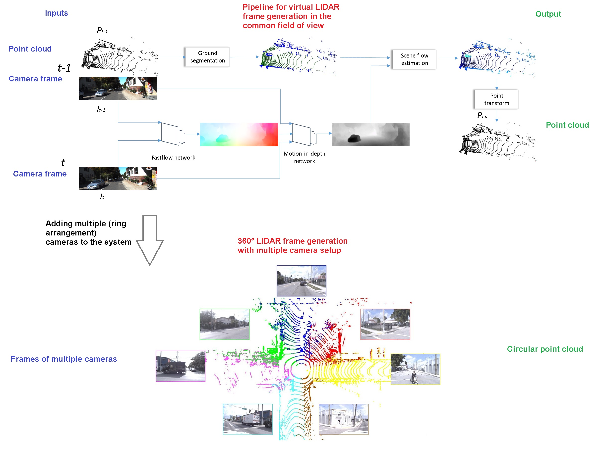
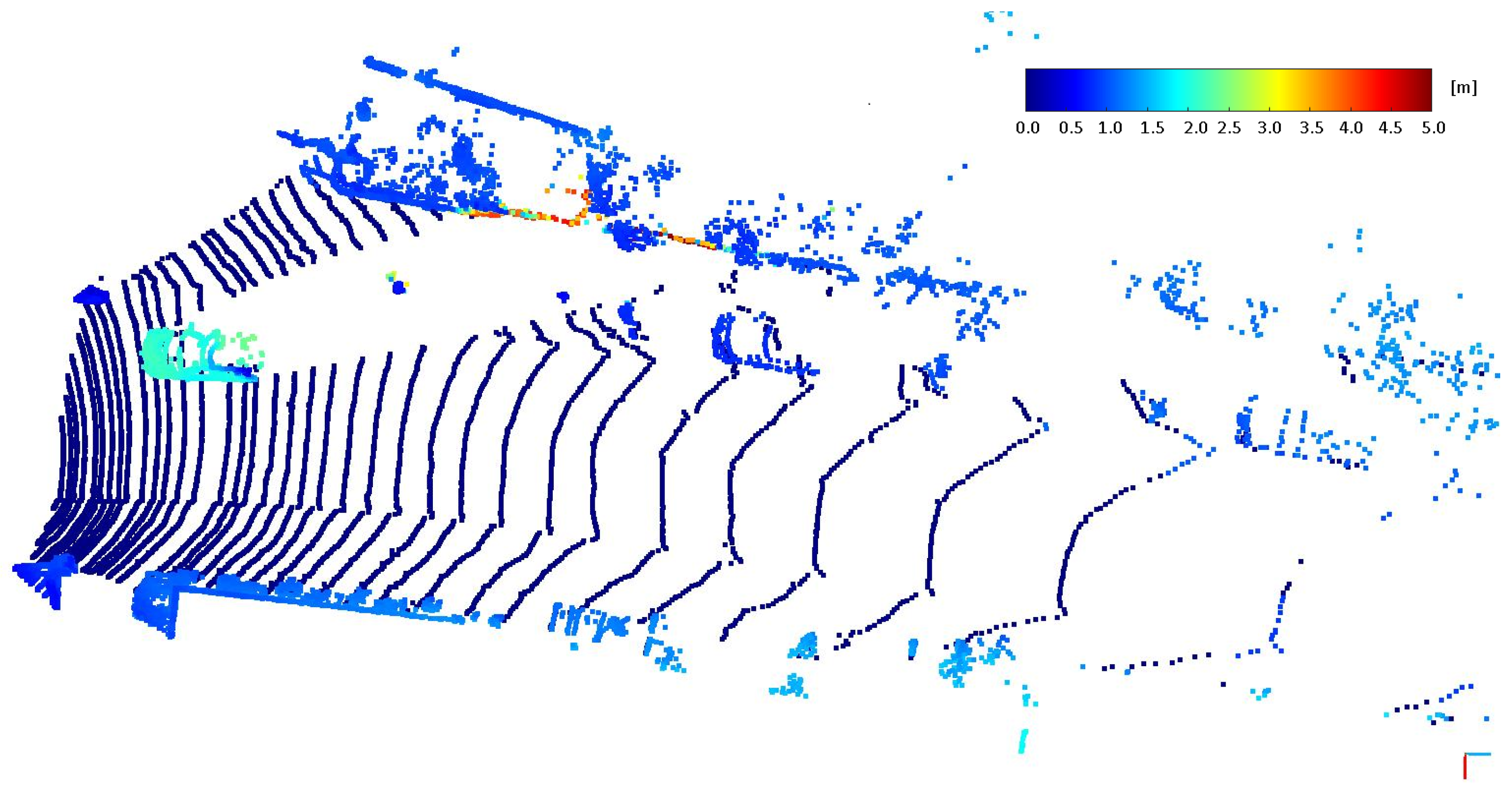
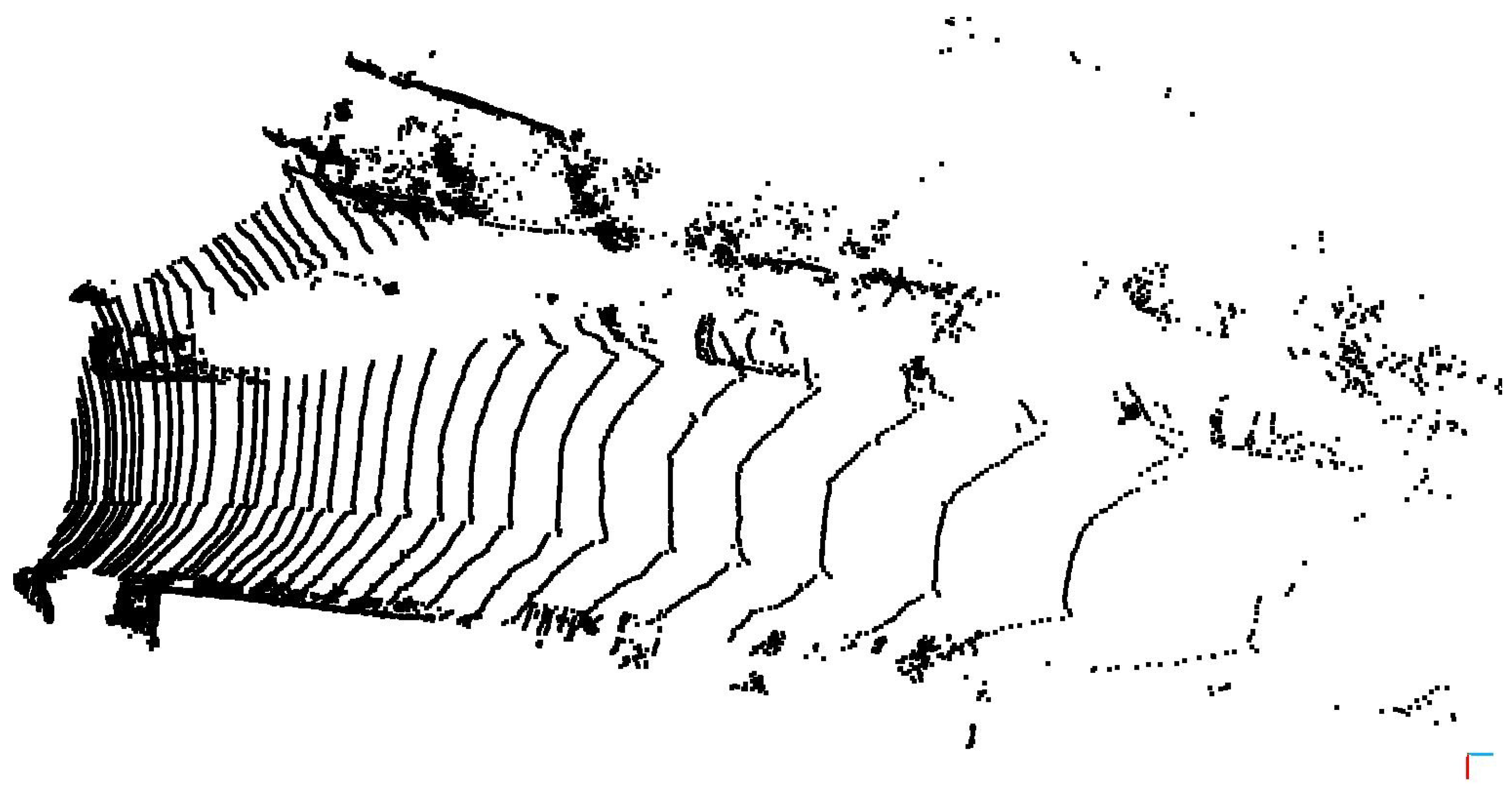
• The pipeline adapts to the point cloud characteristics and generates virtual clouds with similar characteristics to the real measurements. The point-level transformation of the system explains this fact. You can observe that by seeing our result on different LIDAR sensors (e.g., in Figure 2 and Figure in Section 4.2).
• Ego-motion of the vehicle does not need to be known or estimated as in previous works ([7,8]).

Camera measurements in time moments when complete LIDAR frames are not available allow our method to generate virtual point clouds and, in this way, enable the temporal up-sampling. The problem and result are illustrated in Figure 1 and Figure 2.

P and I denote LIDAR and camera measurements, respectively, v index indicates the virtually generated point clouds and t is the timestamp. In the remaining part of the paper, the following notation is used: the data points (with arbitrary dimension) and an array of data points are indicated with the same letter but, in the latter case, it is bolded (e.g., point clouds—$P\in \mathbf{P}$, images—$I\in \mathbf{I}$).

1.1. Contribution

The main contributions of the paper are the following:

• We propose a framework, applying optical principles (flow and expansion) to solve one of the critical problems of autonomous driving researches, namely the balancing between the spatial and temporal resolution of 3D LIDAR measurements.
• We extend the state of the art with a new optical flow calculation method, enabling a real-time run of our system and temporal up-sampling of LIDAR measurements.
• The baseline is enhanced by ground estimation, which ensures higher accuracy of virtual measurement generation.
• Our proposal includes motion vector estimation (point-wise) of surrounding agents (without the requirement of solving the challenging dynamic object segmentation problem [14]). This is a significant advantage compared to alternatives.

1.2. Outline of the Paper

The paper is organized as follows: Section 2 studies the related literature. Section 3 introduces the proposed pipeline. Section 4 shows performance measures from our tests, while Section 5 provides an ablation study and further discussion. Finally, the conclusions are drawn in Section 6.

Figure 1. Illustration of the up-sampling problem and our solution on the Argoverse dataset [15]. In the dataset, camera images of (b) (at timestamp t) exist, but the corresponding LIDAR measurement does not. We generated this (colored) LIDAR point cloud utilizing $P_{t-1}$, $I_{t-1}$ and $I_t$. (a) Lidar ($P_{t-1}$) and camera ($I_{t-1}$) measurements at timestamp $t-1$. (b) Camera measurements ($I_t$) at timestamp t and the generated virtual LIDAR measurement ($P_{t,v}$) to the given time moment. Colormap around the camera images and in the point cloud indicates which image (with a common field of view) was used to generate the given point cloud part.

Figure 1. Illustration of the up-sampling problem and our solution on the Argoverse dataset [15]. In the dataset, camera images of (b) (at timestamp t) exist, but the corresponding LIDAR measurement does not. We generated this (colored) LIDAR point cloud utilizing $P_{t-1}$, $I_{t-1}$ and $I_t$. (a) Lidar ($P_{t-1}$) and camera ($I_{t-1}$) measurements at timestamp $t-1$. (b) Camera measurements ($I_t$) at timestamp t and the generated virtual LIDAR measurement ($P_{t,v}$) to the given time moment. Colormap around the camera images and in the point cloud indicates which image (with a common field of view) was used to generate the given point cloud part.

Figure 2. Details of the virtual point cloud generated with inputs visible in Figure 1. Colormap: Green—$P_{t-1}$ (last available measurement), Blue—$P_{t,v}$ (generated point cloud) and Red—$P_{t+1}$ (future point cloud, only serves illustration purposes). Looking into the enlarged part of the point clouds, it is visible that both dynamic and static objects occupy intermediate positions (in terms of position and orientation) in t (the timestamp of the generation) relative to $t-1$ and $t+1$, as was expected.

Figure 2. Details of the virtual point cloud generated with inputs visible in Figure 1. Colormap: Green—$P_{t-1}$ (last available measurement), Blue—$P_{t,v}$ (generated point cloud) and Red—$P_{t+1}$ (future point cloud, only serves illustration purposes). Looking into the enlarged part of the point clouds, it is visible that both dynamic and static objects occupy intermediate positions (in terms of position and orientation) in t (the timestamp of the generation) relative to $t-1$ and $t+1$, as was expected.

2. Related Works

This section is divided into four subsections. First, spatial up-sampling of point clouds is investigated, as it has mature methods and is similar to our approach in terms of sensor fusion. Second, future frame prediction literature is introduced, which is a recent research interest and similar to our approach as it aims for the virtual LIDAR frame generation but ignores actual information. Third, LIDAR frame interpolation methods are examined, which have the same purpose as our approach but they can be applied offline, as they require a ’future’ frame for the generation of in-between frames. Finally, some earlier approaches for temporal up-sampling are discussed.

2.1. Spatial Up-Sampling

The spatial up-sampling of LIDAR point clouds is usually driven by camera images. These methods aim to estimate depth for every pixel of a depth image having the same resolution as a corresponding RGB image with an input very sparse depth image initialized with projected LIDAR data points. That is why this problem is commonly referred to as depth completion [16]. As the targeted resolution comes from an image, images help (with a few exceptions, e.g., [17,18] or [19] for special sensor characteristics) in the process of pixel-wise depth estimation. There are different approaches to performing this, such as semantic-based up-sampling [20], but deep-learning-based methods (e.g., [5,6]) are currently the most successful ones. These methods inspire our solution to the temporal up-sampling problem in the sense that our approach is also camera-driven, we utilize richer camera information to do the up-sampling and we expect the output to be the same (temporal) resolution as the corresponding camera has.

2.2. Point Cloud Prediction

Point cloud prediction or sequential point cloud forecasting is a hot research topic. The methods of solving this problem are important to our research. They also generate virtual point clouds, as our proposal uses previous frame information. In this way, they can be alternatives to the pipeline we propose. However, they aim differently; they try to predict the future. That is why they have a different approach, too. They do not use current (camera) information, which even theoretically limits their accuracy. Furthermore, these typically neural-network-based methods (such as [12,13,21,22] or [23]) have other drawbacks too:

• As several previous frames are necessary for the prediction (usually 5), it implies that the motion model is embedded in the system resulting in a loss of generality.
• End-to-end training of point cloud prediction could result in weak robustness against different datasets and point cloud characteristics.
• Most of these methods operate only near real time and in close range.

We present a comparison in Section 4 to prove our superiority to these types of methods in the temporal up-sampling problem.

2.3. Point Cloud Interpolation

Point cloud interpolation methods such as [10,11,24,25] have similar intermediate aims to ours, namely generating virtual LIDAR frames between two real LIDAR measurements. However, they have a final goal, offering a solution to the frequency mismatching problem of LIDAR and cameras, which is very distinct from ours. In this way, these methods cannot be applied to our problem. They work offline, as they utilize frames from time $t+1$, naturally not available at time moment t, to generate measurements to timestamp t. Still, we outperform these offline methods in certain performance measures (see Section 4).

These methods may be used as preprocessing to ours if the synchronization of camera and LIDAR is not solved; in practice, in most cases, using camera frames closest in time to the LIDAR frame is considered accurate enough. Thus, offline interpolation is optional. Offline interpolation cannot be an alternative to our proposal in autonomous driving, while we provide an online substitute for these methods.

2.4. Temporal Up-Sampling

Temporal up-sampling of measurements is not completely unknown to the literature [26], yet, there are only very few studies available trying to solve the temporal up-sampling problem of point clouds. Ref. [9] refers to the temporal up-sampling problem as predicting future Pseudo-LIDAR frames, which could be directly used as an alternative to our proposal. However, they require three camera frames as input and two previous LIDAR frames. The only method which only needs two camera frames and one previous LIDAR frame (as the one proposed here) is published in [7,8]. In [27], a motion-in-depth estimation network is proposed using two camera frames. This method cannot be directly applied to the temporal up-sampling problem. However, it should be mentioned here as we extended this method to be applicable to the given issue. Comparisons to these methods are presented in Section 4.

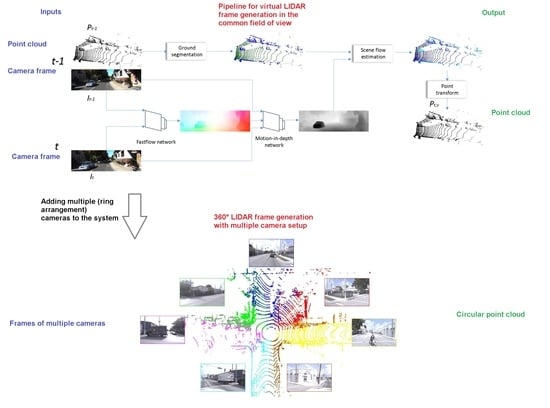
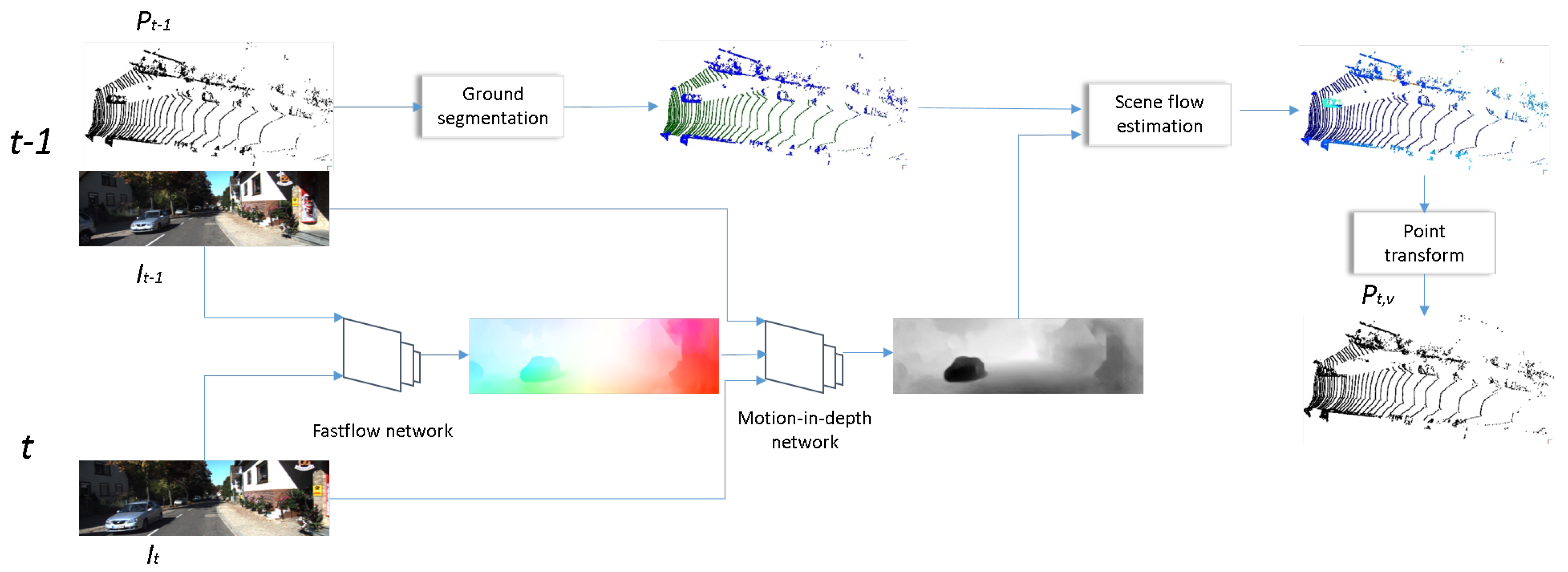
3. The Proposed Method

From here, we focus on describing the generation of only one virtual point cloud measurement. As we can generate virtual measurements to any t time moment (with camera measurement), the following steps can be repeated as many times as you want, resulting in a temporally upscaled point cloud stream.

The proposed pipeline has five important steps and these are the following:

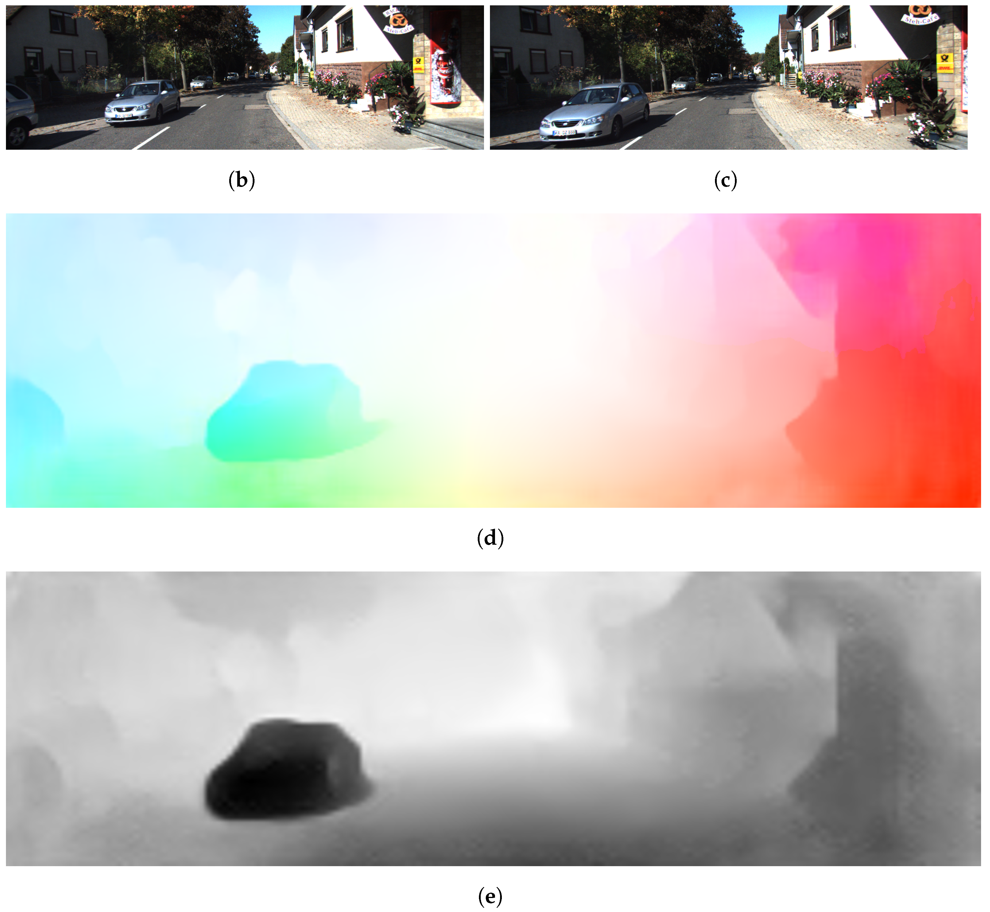
• Estimate optical flow ($\tilde{u}$) between images acquired at $t-1$ and t;
• Estimate optical expansion (s) and motion in depth ($\tau =\frac{1}{s}$) from the previously estimated flow;
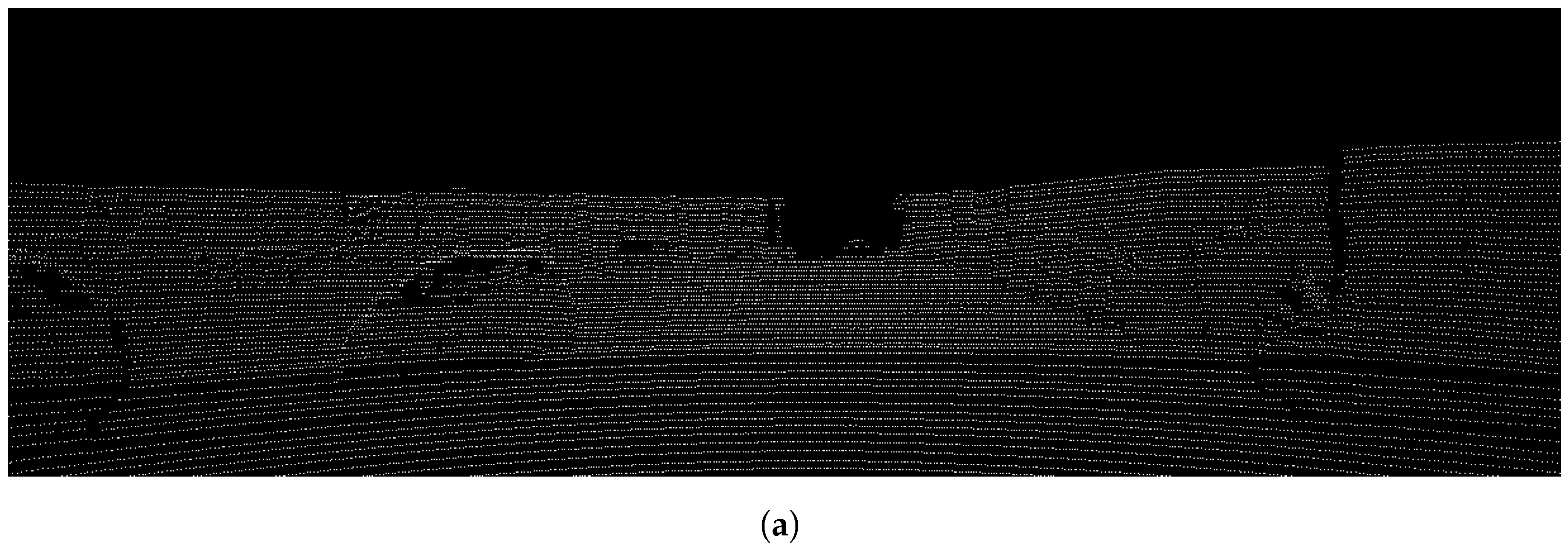
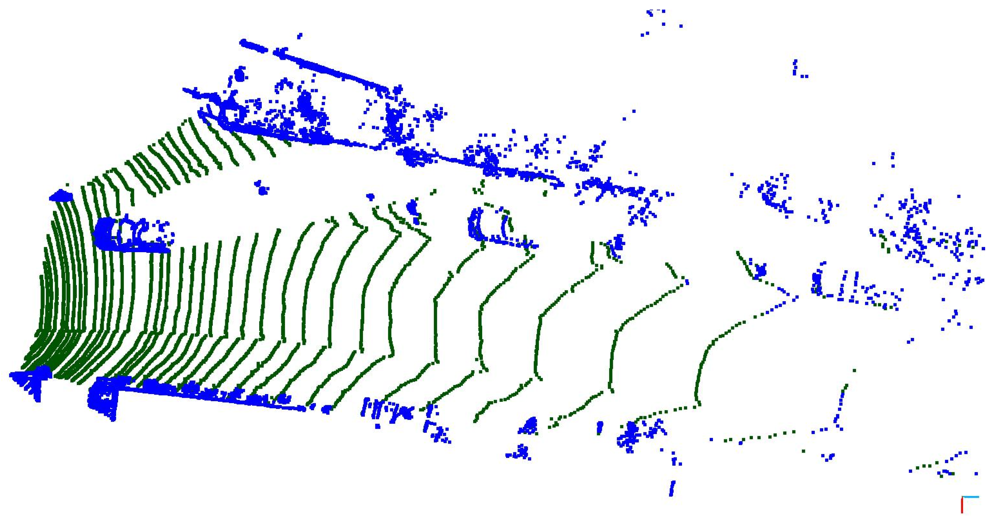
• Estimate ground model and points on $P_{t-1}$;
• Calculate scene flow, utilizing the estimations and LIDAR measurements from $t-1$;
• Transform the object points with the estimated scene flow to generate the virtual measurement ($P_{t,v}$) at t.

The differences from the baseline [27] are in steps 1 and 3–5; in step 2 we utilize their network for motion-in-depth estimation. In step 1, utilizing FastFlowNet enables real-time application. Step 3 and utilizing it in step 4 (also applying the exact formula in step 5) increases the similarity to real measurements (further details in Table in Section 5.3). One of the biggest advantage of our pipeline compared to alternatives (e.g., [8]) is that differentiating static and moving object is unnecessary; movement calculation of surrounding agents is included.

The pipeline is illustrated in Figure 3 for the inputs of Figure 4. Before using it, the camera intrinsic [28] and camera–LIDAR (extrinsic) [29] calibration should be executed. The depth images containing $Z_{t-1}$ values are determined using the LIDAR–camera $T_{L,C}$ transformation and $\mathbf{K}$ intrinsic matrix. For better visualization, the $t-1$ LIDAR depth measurements are converted to disparity image and illustrated here ($d=\frac{b*f}{Z}$ with b baseline and f focal length).

The intermediate results of the pipeline of this given example will be shown enlarged in the detailed explanation part.

3.1. Optical Flow Estimation

The flow field describes the velocity of image pixels as:

$$\tilde{u}={[u,v]}^T=p_t-p_{t-1}={[x_t,y_t]}^T-{[x_{t-1},y_{t-1}]}^T,$$

(1)

where u and v are the flow components, between $p_t$ and $p_{t-1}$ image points of different time stamps with x and y as the pixel coordinates.

We adapt FastFlowNet [30] to estimate the optical flow field. FastFlowNet is a lightweight model for fast and accurate prediction with only 1.37 M parameters enabling a real-time run. It uses a coarse-to-fine paradigm with a head-enhanced pooling pyramid (HEPP) feature extractor to intensify high-resolution pyramid features while reducing parameters. In addition, the center dense dilated correlation (CDDC) layer is applied to compact cost volume that can keep a large search radius with reduced computation time and a shuffle block decoder (SBD) is implemented into pyramid levels to accelerate the estimation. Further details can be found in the original paper [30]. Illustration of a resulted flow field colored according to the Middlebury color code [31] with input images of Figure 4 can be seen in Figure 4d.

3.2. Motion-in-Depth Estimation

Motion-in-depth, by definition, is:

$$\tau =\frac{Z_t(p_{t-1}+\tilde{u}\left(p_{t-1}\right))}{Z_{t-1}\left(p_{t-1}\right)},$$

(2)

where $Z_t$ and $Z_{t-1}$ are the depth values at time moments t and $t-1$, respectively. In this step, we estimate an ’image’ of depth ratios which will relate our 2D flow estimations to a 3D motion estimation (as we see later). Optical expansion (in case of not rotating scene elements and orthographic camera model) is the reciprocal of the motion-in-depth (see further details in [27]). Thus, if we can estimate the scale change of the scene elements, we will ascertain how much they moved closer or farther away. This principle is utilized in the work [27] where local affine transformation was used to estimate scale changes:

$$(p_t-p_{t,c})=\mathbf{A}(p_{t-1}-p_{t-1,c}),$$

(3)

$$\tau =\frac{1}{\sqrt{|det\mathbf{A}|}},$$

(4)

where $\mathbf{A}$ is ${\mathbb{R}}^{2\times 2}$ matrix describing the local affine transformation and c index indicates a center pixel of a given coordinate; $p_t$ and $p_{t-1}$, corresponding pixels of images acquired at different time stamps, are related by Equation (1).

Later on, the estimated scale ratios were used to train a network for the estimation of depth change. We applied this network to get motion-in-depth estimations. The image generated from the motion-in-depth estimation is illustrated in Figure 4e.

3.3. Ground Model Estimation

Ground model estimation is applied for the following reason: finding the corresponding locations of points of $P_{t-1}$ at time t (estimating 3D scene flow) differs from the problem of estimating LIDAR measurement at time t. Due to the movements and sensor characteristics, the objects will be hit by the sensor in different parts. This will mean a big difference between the scene flow estimated points and real measurements in the case of the ground and far points. (The phenomena can be observed, e.g., in the last column of Figure in Section 4.2 and the importance of our compensation in Table in Section 5.3). So, in our solution, we estimate a ground model and, for the ground points, no displacement is applied. This is based on the assumption that, as we move on the plane and measure, the sensor characteristics (laser emitting angles) do not change. Thus, we will find points approximately at the same distances on this plane. (A more complex model could be applied; however, this simple assumption proved to be useful, accurate and efficient.)

MLESAC [32], a variant of the RANSAC (RANdom SAmple Consensus) robust model-fitting method, is applied to fit a ground plane to the LIDAR points of $P_{t-1}$ with a reference normal vector of ${\left[010\right]}^T$ in camera coordinate system. A 0.2 m threshold was used to define inlier points of the given ground plane.

Estimated ground points are illustrated in Figure 5.

3.4. Calculate 3D Scene Flow

As in [33] 3D scene flow is defined as the three-dimensional motion of 3D points, just as optical flow is the 2D motion of points in an image. For further explanation see [33]. Utilizing the estimated optical flow, the motion-in-depth values and the depths, $Z_{t-1}$ (projected from the LIDAR), the corresponding depth values, $Z_t$, can be determined by rearranging the following Equation [27]:

$$\tilde{U}=P_t-P_{t-1}={\mathbf{K}}^{-1}(Z_t{p}_t-Z_{t-1}{p}_{t-1})=Z_{t-1}{\mathbf{K}}^{-1}(\tau (\tilde{u}+p_{t-1})+p_t),$$

(5)

where $\tilde{U}$ is the 3D scene flow. The displacement ($|\tilde{U}|$) estimated from the 3D scene flow ($\tilde{U}$) is illustrated in Figure 6.

3.5. Generating Virtual Point Cloud

The virtual point cloud to time t is generated from the points of $P_t$ by the following rule:

$${\mathbf{P}}_{t,v}=\left\{\begin{array}{cc}{\mathbf{P}}_{t-1},\hfill & \mathrm{if}{P}_{t-1}^i\in {\mathbf{G}}_t\hfill \\ {\mathbf{P}}_{t-1}+\tilde{U},\hfill & \mathrm{otherwise}\hfill \end{array}\right.,$$

(6)

where the upper index i indicates the $i^{th}$ point of the point cloud and $\mathbf{G}$ represents ground points in the point cloud $\mathbf{P}$. The above equation means that scene flow is only applied for non-ground points (as it is visible in the case of Figure 6). As 3D scene flow is estimated for each point, movement estimation of moving objects is included in the pipeline and we do not have to consider them separately. All the points of static objects should have the same scene flow value (the ego-motion vector in opposite direction), and points of a dynamic object should have some other value (same for the same objects). The resulting point cloud is illustrated in Figure 7. The appropriate estimation of static and moving objects can be observed in Figure 7, where approaching vehicle points have about 2 m estimated displacement. In comparison, static environment points (including parking cars) have a roughly 1 m estimated displacement.

By repeating all the steps listed here for every t without LIDAR measurement (but with camera measurement), a temporally up-sampled point cloud sequence is produced.

4. Results

Here, we provide a quantitative and qualitative evaluation of the proposed pipeline.

4.1. Data for Comparison

Ground truth is unavailable for generating point clouds to time stamps without measurement. That is why we generated point clouds to time stamps with measurements (as others in similar problems). This means that for a sequence with x (number of frames) LIDAR frame, we can generate $x-1$ point clouds and compare it to the real measurements. As different competitors used different datasets with different conditions to evaluate their method, we also used more of them for a fair comparison. Section 4.2 describes the evaluation procedure and introduces our results in the case of the Odometry dataset with qualitative examples and Section 4.3 in the case of the Depth Completion dataset. In our tests, the most commonly applied error metrics for point cloud generation are involved, namely Chamfer Distance (CD) and Earth Movers Distance (EMD). As the literature used different EMDs, we define them in the subsections. The formula of CD is as follows:

$$CD=\frac{1}{N}\sum _{p_{t,v}\in {\mathbf{P}}_{t,v}}\underset{P_t\in {\mathbf{P}}_t}{min}\parallel P_t-P_{t,v}{\parallel }^2+\frac{1}{N}\sum _{P_t\in {\mathbf{P}}_t}\underset{{\mathbf{P}}_{t,v}\in {\mathbf{P}}_{t,v}}{min}{\parallel P_t-P_{t,v}\parallel }^2,$$

(7)

where $P_{t,v}\in {\mathbb{R}}^{N_{t,v}\times 3}$ and $P_t\in {\mathbb{R}}^{N_t\times 3}$ are the data points of the predicted (virtual) ${\mathbf{P}}_{t,v}$ and ground truth ${\mathbf{P}}_t$ point clouds, respectively. The number of generated points ($N_{t,v}$) can differ from the number of data points of the ground truth $N_t$. That is why the denser point cloud is randomly down-sampled to N for these scenarios, where $N=min(N_{t,v},N_t$).

4.2. Odometry Dataset

Papers have used the KITTI Odometry dataset [34] for evaluation and down-sampled the LIDAR frames to 16,384 data points. We also did that and, after that, we only considered data points for which the proposed up-sampling is applied (points seen by camera no. 2). Sequences 08–10 (altogether 6863 frames) were used for testing. The definition of Earth Movers Distance is as follows:

$$EMD=\frac{1}{N}\sum _{P_t\in {\mathbf{P}}_t}{\parallel P_t-\varphi \left(P_{t,v}\right)\parallel }^2,$$

(8)

where $\varphi$ is bijection, which calculates the point-to-point mapping between two point cloud ${\mathbf{P}}_t$ and ${\mathbf{P}}_{t,v}$.

EMD measures the similarity between point clouds by calculating the cost of the global matching problem. For EMD, the approximation of [35] is applied, which is used by [36] and other literature.

The results of our proposed pipeline in the dataset compared to other methods are shown in

Table 1. Quantitative evaluation and comparison of the proposed pipeline on KITTI Odometry dataset. The values of the best-performing methods in case of different measures are bolded.

Methods	Application	CD [m${}^2$]	EMD [m${}^2$]
MoNet (LSTM) [13]	Forecasting	0.573	91.79
MoNet (GRU) [13]	Forecasting	0.554	91.97
SPINet [11]	Offline Interpolation	0.465	40.69
PointINet [10]	Offline Interpolation	0.457	39.46
Rigid body based up-sampling [8]	Online Interpolation	0.471	33.98
Proposed pipeline	Online Interpolation	0.486	28.51

.

In the case of CD, PointINet [10] performed best; however, it cannot be applied online as it needs a ’future frame’ for operation. From the alternatives, rigid body-based up-sampling [8] performed slightly better. We achieved the best performance in the case of EMD, which describes the similarity of point cloud distributions the best.

In the following, we illustrate our method’s state-of-the-art performance through qualitative examples. These can be seen in Figure 8, Figure 9 and Figure 10.

The first columns of the example figures show the generated point clouds from a distance and the columns afterward contain zoomed parts. The following can be observed in Figure 8: the point clouds of the vehicles are less accurate in the case of [8] and about the same accuracy in the case of [27] and our proposal (last row). However, regarding the accuracy of ground points, our recommendation is the best (last column). In Figure 9, the static scene (second column) is estimated with the most considerable precision with [8] (using ego-motion estimation) but ours are almost as good; Ref. [27] is the worst of the three. The dynamic points of far vehicles (third column) are the most precise in the case of our proposal. Figure 10 illustrates a further example where the limitation of the proposal can be seen (ground model fitting limits the precision of generated ground points). However, dynamic object parts are still the most accurate with our proposal.

4.3. Depth Completion Dataset

As other competitors used the Depth Completion Dataset [16] for evaluation, we tested our proposal on this, too, on the validation subset containing 1000 frames. The performance measuring procedure (used by [9] and others) does not include down-sampling. (Down-sampling is usually used for faster calculation of the measures.) However, in this case, only points considered in the field of view of the camera image are cropped to 1216 × 256 pixel resolution (leaving out distant points). The Earth Movers definition applied by [9] is the following (without squared norm):

$$EMD=\frac{1}{N}\sum _{P_t\in {\mathbf{P}}_t}\parallel P_t-\varphi \left(P_{t,v}\right)\parallel ,$$

(9)

Our results compared to other methods are in

Table 2. Quantitative evaluation and comparison of the proposed pipeline on KITTI depth completion dataset. The values of the best-performing methods in case of different measures are bolded.

Methods	Application	CD [m${}^2$]	EMD [m]
Prediction [22]	Forecasting	0.202	11.498
PLIN [24]	Offline Interpolation	0.21	-
PLIN+ [25]	Offline Interpolation	0.12	-
Future pseudo-LIDAR [9]	Online Interpolation	0.157	3.303
Proposed pipeline	Online Interpolation	0.141	0.806

.

One can see that, in the case of CD, Ref. [25] performed the best; however, this method cannot be applied to our problem in practice, as it needs a future point cloud. Apart from that, our proposed pipeline has the best performance in both measures.

5. Discussion

This section contains further discussion beyond our test results provided in the previous section. First, the computation efficiency discussion; next, a separate evaluation for dynamic objects is presented, and, finally, an ablation study is presented.

5.1. Computation Efficiency

Real-time running is essential as our goal is to temporally up-sample point clouds. (As a matter of fact, the run time should be less than the time elapsed between measurements with a given frequency we aim to up-sample.) The running time of the pipeline components is listed in

Table 3. Average running time of the different pipeline components.

Component	Average Running Time [ms]
Optical flow estimation	14
Motion-in-depth estimation	29
Ground estimation	8
Frame generation (scene flow + transformation)	≈0
Total	51

with the following configuration: Intel Core i7-4790K @ 4.00 GHz processor, 32 GB RAM, Nvidia GTX 1080 GPU, Windows 10 64 bit. For the tests, KITTI-sized images were used (about 1200 × 350 resolution).

As the total running time of the system is 51 ms, we can generate virtual point clouds with almost 20 Hz, meaning we can up-sample 5 and 10 Hz LIDAR measurements with the current limited research configuration. In

Table 4. Running time of different methods with the type of the GPU on which it is measured. The running time value of the best-performing method is bolded.

Methods	GPU	Average Running Time [ms]
Future pseudo-LIDAR [9]	Nvidia RTX 2080Ti	52
Rigid body based up-sampling [8]	Nvidia GTX 1080	62
Proposed method	Nvidia GTX 1080	51

, our method is compared to alternatives that can run in real time and have similar inputs and the same goal as us, namely up-sampling point cloud measurements.

As shown in Table 4, we outperform the alternatives in terms of running time (even without considering our GPU disadvantage).

5.2. Dynamic Objects

We made an evaluation separately only for dynamic objects as in [8]. There are two main reasons why this is important to investigate:

• The ego-motion can be determined with different localization sensors (such as in [37]) or by methods (such as [38]), and the motion of static scene elements can be calculated based on that. However, for dynamic objects, we cannot do that.
• Dynamic objects generally pose a greater threat as they change their position and they also can change their state variables (angular and linear velocity, acceleration).

For the evaluation, we used the annotations of the Semantic KITTI dataset [39] to select vehicles as dynamic object candidates on the sequences of 08–10. The evaluation results can be observed in

Table 5. Quantitative evaluation and comparison of the proposed pipeline on KITTI Odometry dataset (just vehicles). The values of the best-performance methods in case of different measures are bolded.

Methods	CD [m${}^2$]	EMD [m${}^2$]
Point based [12]	2.37	211.47
Range map based [12]	0.92	128.81
Rigid body based up-sampling [8]	0.63	31.03
Proposed pipeline	0.26	17.50

.

As Table 5 shows, we provide the best performance in the case of generating point clouds of dynamic objects.

5.3. Ablation Study

Here, we provide an ablation study to prove the significance of our contributions. It can be seen in table form in

Table 6. Ablation study on KITTI Odometry dataset. The values of the best-performance are bolded.

Components	CD [m${}^2$]	EMD [m${}^2$]	Runtime [ms]
Proposed pipeline	0.486	28.51	51
Without ground estimation	0.508	34.50	43
Without FastFlowNet	0.508	34.40	95
Baseline (appr.) [27]	0.547	34.39	270

. The extensions to the baselines are enhanced error metrics or running time of the algorithm, or both.

In Table 6, Baseline (appr.) stands for the demonstration code provided by the authors of [27]. Appr. abbreviates approximation as the authors in their demo code used the approximation of $Z_t\left(p_{t-1}\right)=\tau Z_{t-1}\left(p_{t-1}\right)$ ignoring $\tilde{u}$ in position (see Equation (2)). ’Without FastFlowNet’ means our development where the exact equation is used (reducing errors) and, also, the runtime is decreased as we optimized the code handed out by taking a grid generation step out of the network. This run time is more closely reported by [27]. ‘Without ground estimation’ indicates our extension using FastFlowNet instead of the Volumetric Correspondence Networks (VCN) [40]; it is a very significant reduction in the runtime, making the up-sampling possible. Our proposed pipeline is the one described in this paper, using both the optical flow estimation and the ground model estimation. Adding the ground estimation step somewhat increased the runtime; however, there was a significant improvement in the error metrics.

6. Conclusions

We introduced a methodology to solve the problem of temporally up-sampling LIDAR point clouds utilizing a mono camera. We extended the state of the art to be able to do this in real time. The proposed pipeline has several advantages compared to alternatives; it is not designed for specific point cloud characteristics and it does not require ego-motion estimation. Our evaluation of the KITTI dataset shows that our framework has state-of-the-art accuracy in terms of similarity to real measurements. In the future, we intend to further extend our tests, e.g., with panoramic images, and apply a more sophisticated sensor model to calculate more accurately the point locations of the generated virtual point clouds.

References

- Nagy, B.; Benedek, C. On-the-Fly Camera and Lidar Calibration. Remote Sens. 2020, 12, 1137. [Google Scholar] [CrossRef]
- Chen, Z.; Zhang, J.; Tao, D. Progressive LiDAR adaptation for road detection. IEEE/CAA J. Autom. Sin. 2019, 6, 693–702. [Google Scholar] [CrossRef]
- Wu, X.; Peng, L.; Yang, H.; Xie, L.; Huang, C.; Deng, C.; Liu, H.; Cai, D. Sparse Fuse Dense: Towards High Quality 3D Detection with Depth Completion. In Proceedings of the IEEE/CVF Conference on Computer Vision and Pattern Recognition (CVPR), New Orleans, LA, USA, 18–24 June 2022; pp. 5418–5427. [Google Scholar]
- Liu, Z.; Xiao, X.; Zhong, S.; Wang, W.; Li, Y.; Zhang, L.; Xie, Z. A feature-preserving framework for point cloud denoising. Comput.-Aided Des. 2020, 127, 102857. [Google Scholar] [CrossRef]
- Zhao, S.; Gong, M.; Fu, H.; Tao, D. Adaptive Context-Aware Multi-Modal Network for Depth Completion. IEEE Trans. Image Process. 2021, 30, 5264–5276. [Google Scholar] [CrossRef]
- Hu, M.; Wang, S.; Li, B.; Ning, S.; Fan, L.; Gong, X. PENet: Towards Precise and Efficient Image Guided Depth Completion. In Proceedings of the 2021 IEEE International Conference on Robotics and Automation (ICRA), Xi’an, China, 30 May–5 June 2021; pp. 13656–13662. [Google Scholar] [CrossRef]
- Rozsa, Z.; Sziranyi, T. Temporal Up-Sampling of LIDAR Measurements Based on a Mono Camera. In Image Analysis and Processing—ICIAP 2022, Proceedings of the 21st International Conference on Image Analysis and Processing, Lecce, Italy, 23–27 May 2022; Sclaroff, S., Distante, C., Leo, M., Farinella, G.M., Tombari, F., Eds.; Springer International Publishing: Cham, Switzerland, 2022; pp. 51–64. [Google Scholar]
- Rozsa, Z.; Sziranyi, T. Virtually increasing the measurement frequency of LIDAR sensor utilizing a single RGB camera. arXiv 2023, arXiv:2302.05192. [Google Scholar]
- Huang, X.; Lin, C.; Liu, H.; Nie, L.; Zhao, Y. Future Pseudo-LiDAR Frame Prediction for Autonomous Driving. Multimed. Syst. 2022, 28, 1611–1620. [Google Scholar] [CrossRef]
- Lu, F.; Chen, G.; Qu, S.; Li, Z.; Liu, Y.; Knoll, A. PointINet: Point Cloud Frame Interpolation Network. In Proceedings of the Thirty-Fifth AAAI Conference on Artificial Intelligence, Online, 2–9 February 2021. [Google Scholar]
- Xu, J.; Le, X.; Chen, C. SPINet: Self-supervised point cloud frame interpolation network. Neural Comput. Appl. 2022, 35, 9951–9960. [Google Scholar] [CrossRef]
- Weng, X.; Wang, J.; Levine, S.; Kitani, K.; Rhinehart, N. Inverting the Pose Forecasting Pipeline with SPF2: Sequential Pointcloud Forecasting for Sequential Pose Forecasting. In Proceedings of the (CoRL) Conference on Robot Learning, Online, 16–18 November 2020. [Google Scholar]
- Lu, F.; Chen, G.; Li, Z.; Zhang, L.; Liu, Y.; Qu, S.; Knoll, A. MoNet: Motion-Based Point Cloud Prediction Network. IEEE Trans. Intell. Transp. Syst. 2021, 23, 13794–13804. [Google Scholar] [CrossRef]
- Chen, X.; Li, S.; Mersch, B.; Wiesmann, L.; Gall, J.; Behley, J.; Stachniss, C. Moving Object Segmentation in 3D LiDAR Data: A Learning-based Approach Exploiting Sequential Data. IEEE Robot. Autom. Lett. (RA-L) 2021, 6, 6529–6536. [Google Scholar] [CrossRef]
- Chang, M.F.; Lambert, J.; Sangkloy, P.; Singh, J.; Bak, S.; Hartnett, A.; Wang, D.; Carr, P.; Lucey, S.; Ramanan, D.; et al. Argoverse: 3D Tracking and Forecasting with Rich Maps. In Proceedings of the IEEE/CVF Conference on Computer Vision and Pattern Recognition (CVPR), Long Beach, CA, USA, 15–20 June 2019. [Google Scholar] [CrossRef]
- Uhrig, J.; Schneider, N.; Schneider, L.; Franke, U.; Brox, T.; Geiger, A. Sparsity Invariant CNNs. In Proceedings of the 2017 International Conference on 3D Vision (3DV), Qingdao, China, 10–12 October 2017. [Google Scholar] [CrossRef]
- Premebida, C.; Garrote, L.; Asvadi, A.; Ribeiro, A.; Nunes, U. High-resolution LIDAR-based depth mapping using bilateral filter. In Proceedings of the 2016 IEEE 19th International Conference on Intelligent Transportation Systems (ITSC), Rio de Janeiro, Brazil, 1–4 November 2016; pp. 2469–2474. [Google Scholar] [CrossRef]
- Ku, J.; Harakeh, A.; Waslander, S.L. In Defense of Classical Image Processing: Fast Depth Completion on the CPU. In Proceedings of the 2018 15th Conference on Computer and Robot Vision (CRV), Toronto, ON, Canada, 8–10 May 2018; pp. 16–22. [Google Scholar] [CrossRef]
- Zováthi, Ö.; Pálffy, B.; Jankó, Z.; Benedek, C. ST-DepthNet: A spatio-temporal deep network for depth completion using a single non-repetitive circular scanning Lidar. IEEE Robot. Autom. Lett. 2023, 8, 3270–3277. [Google Scholar] [CrossRef]
- Schneider, N.; Schneider, L.; Pinggera, P.; Franke, U.; Pollefeys, M.; Stiller, C. Semantically Guided Depth Upsampling. In Pattern Recognition, Proceedings of the 38th German Conference on Pattern Recognition, Hannover, Germany, 12–15 September 2016; Springer International Publishing: Cham, Switzerland, 2016; Volume 9796, pp. 37–48. [Google Scholar] [CrossRef]
- Wencan, C.; Ko, J.H. Segmentation of Points in the Future: Joint Segmentation and Prediction of a Point Cloud. IEEE Access 2021, 9, 52977–52986. [Google Scholar] [CrossRef]
- Deng, D.; Zakhor, A. Temporal LiDAR Frame Prediction for Autonomous Driving. In Proceedings of the 2020 International Conference on 3D Vision (3DV), Fukuoka, Japan, 25–28 November 2020; IEEE Computer Society: Los Alamitos, CA, USA, 2020; pp. 829–837. [Google Scholar]
- He, P.; Emami, P.; Ranka, S.; Rangarajan, A. Learning Scene Dynamics from Point Cloud Sequences. Int. J. Comput. Vis. 2022, 130, 1–27. [Google Scholar] [CrossRef]
- Liu, H.; Liao, K.; Zhao, Y.; Liu, M. PLIN: A Network for Pseudo-LiDAR Point Cloud Interpolation. Sensors 2020, 20, 1573. [Google Scholar] [CrossRef] [PubMed]
- Liu, H.; Liao, K.; Lin, C.; Zhao, Y.; Guo, Y. Pseudo-LiDAR Point Cloud Interpolation Based on 3D Motion Representation and Spatial Supervision. IEEE Trans. Intell. Transp. Syst. 2021, 23, 6379–6389. [Google Scholar] [CrossRef]
- Beck, H.; Kühn, M. Temporal Up-Sampling of Planar Long-Range Doppler LiDAR Wind Speed Measurements Using Space-Time Conversion. Remote Sens. 2019, 11, 867. [Google Scholar] [CrossRef]
- Yang, G.; Ramanan, D. Upgrading Optical Flow to 3D Scene Flow Through Optical Expansion. In Proceedings of the IEEE/CVF Conference on Computer Vision and Pattern Recognition (CVPR), Seattle, WA, USA, 13–19 June 2020. [Google Scholar]
- Zhang, Z. A flexible new technique for camera calibration. IEEE Trans. Pattern Anal. Mach. Intell. 2000, 22, 1330–1334. [Google Scholar] [CrossRef]
- Zhou, L.; Li, Z.; Kaess, M. Automatic Extrinsic Calibration of a Camera and a 3D LiDAR Using Line and Plane Correspondences. In Proceedings of the 2018 IEEE/RSJ International Conference on Intelligent Robots and Systems (IROS), Madrid, Spain, 1–5 October 2018; pp. 5562–5569. [Google Scholar] [CrossRef]
- Kong, L.; Shen, C.; Yang, J. FastFlowNet: A Lightweight Network for Fast Optical Flow Estimation. In Proceedings of the 2021 IEEE International Conference on Robotics and Automation (ICRA), Xi’an, China, 30 May–5 June 2021. [Google Scholar]
- Baker, S.; Scharstein, D.; Lewis, J.; Roth, S.; Black, M.; Szeliski, R. A Database and Evaluation Methodology for Optical Flow. Int. J. Comput. Vis. 2007, 92, 1–31. [Google Scholar] [CrossRef]
- Torr, P.; Zisserman, A. MLESAC: A New Robust Estimator with Application to Estimating Image Geometry. Comput. Vis. Image Underst. 2000, 78, 138–156. [Google Scholar] [CrossRef]
- Vedula, S.; Rander, P.; Collins, R.; Kanade, T. Three-dimensional scene flow. IEEE Trans. Pattern Anal. Mach. Intell. 2005, 27, 475–480. [Google Scholar] [CrossRef]
- Geiger, A.; Lenz, P.; Urtasun, R. Are we ready for Autonomous Driving? The KITTI Vision Benchmark Suite. In Proceedings of the Conference on Computer Vision and Pattern Recognition (CVPR), Providence, RI, USA, 16–21 June 2012. [Google Scholar]
- Bertsekas, D.P. A distributed asynchronous relaxation algorithm for the assignment problem. In Proceedings of the 1985 24th IEEE Conference on Decision and Control, Fort Lauderdale, FL, USA, 11–13 December 1985; pp. 1703–1704. [Google Scholar] [CrossRef]
- Fan, H.; Su, H.; Guibas, L. A Point Set Generation Network for 3D Object Reconstruction from a Single Image. In Proceedings of the 2017 IEEE Conference on Computer Vision and Pattern Recognition (CVPR), Honolulu, HI, USA, 21–26 July 2017; pp. 2463–2471. [Google Scholar] [CrossRef]
- He, L.; Jin, Z.; Gao, Z. De-Skewing LiDAR Scan for Refinement of Local Mapping. Sensors 2020, 20, 1846. [Google Scholar] [CrossRef]
- Campos, C.; Elvira, R.; Gomez, J.J.; Montiel, J.M.M.; Tardos, J.D. ORB-SLAM3: An Accurate Open-Source Library for Visual, Visual-Inertial and Multi-Map SLAM. IEEE Trans. Robot. 2021, 37, 1874–1890. [Google Scholar] [CrossRef]
- Behley, J.; Garbade, M.; Milioto, A.; Quenzel, J.; Behnke, S.; Stachniss, C.; Gall, J. SemanticKITTI: A Dataset for Semantic Scene Understanding of LiDAR Sequences. In Proceedings of the IEEE/CVF International Conference on Computer Vision (ICCV), Seoul, Republic of Korea, 27 October–2 November 2019. [Google Scholar]
- Yang, G.; Ramanan, D. Volumetric Correspondence Networks for Optical Flow. In Proceedings of the NeurIPS 2019-Conference on Neural Information Processing Systems, Vancouver, BC, Canada, 8–14 December 2019. [Google Scholar]