
Lake Turbidity Mapping Using an OWTs-bp Based Framework and Sentinel-2 Imagery


Abstract
1. Introduction
2. Study Region
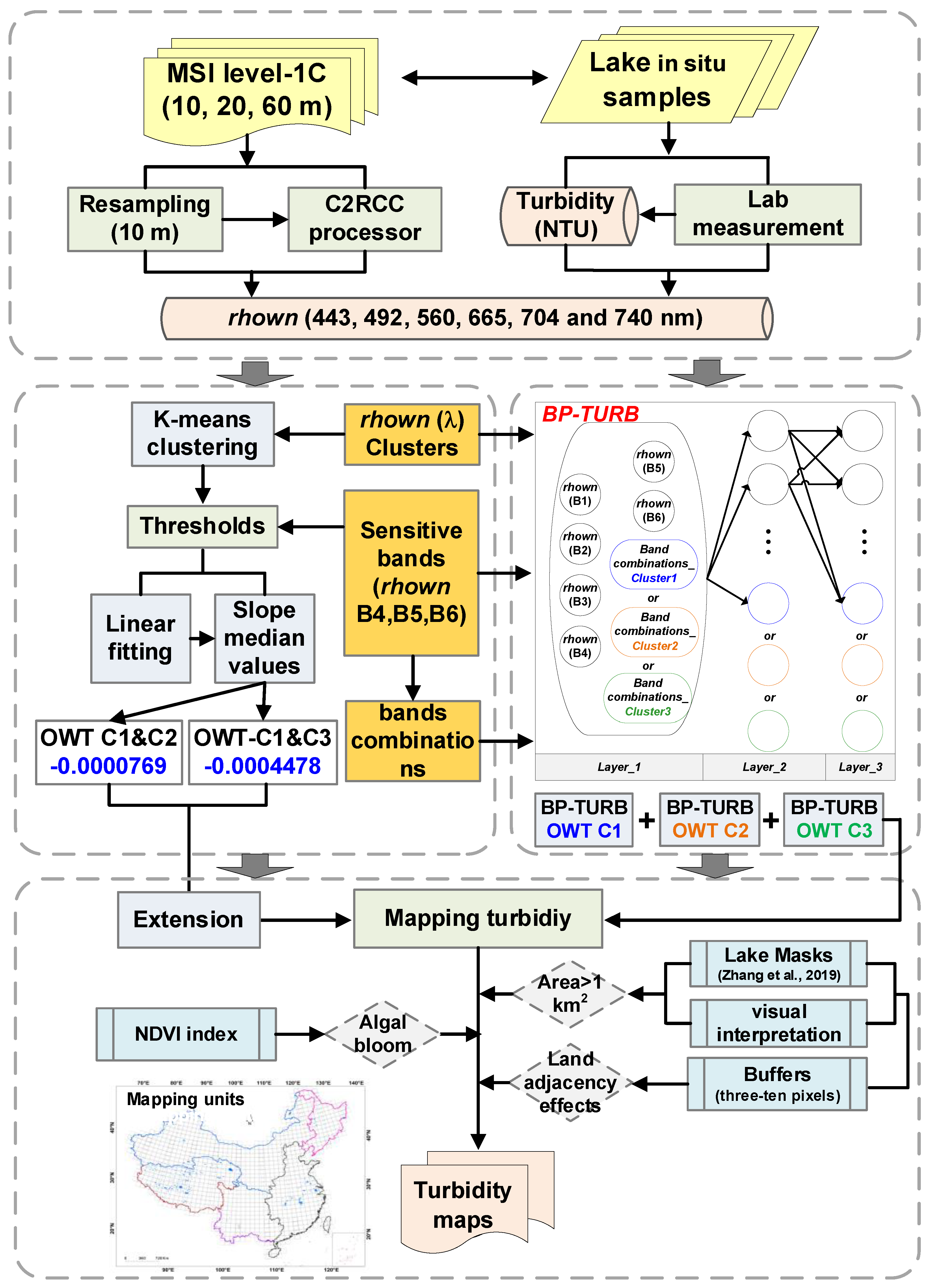
3. Methods
3.1. In Situ Water Quality Collection and Field Measurements
3.2. Water Quality and Light Absorption Determination in Laboratory
3.3. MSI Imagery Match-Ups
3.4. Lake Optical Clustering for Rhown(λ)-Spectra
3.5. Back-Propagation Neural-Turbidity Models (BP-TURB)
3.6. Chinese Turbidity Products
3.7. Data on Abiotic Factors
4. Results
4.1. The Importance of Multi-Spatial-Temporal In Situ Water Qualities
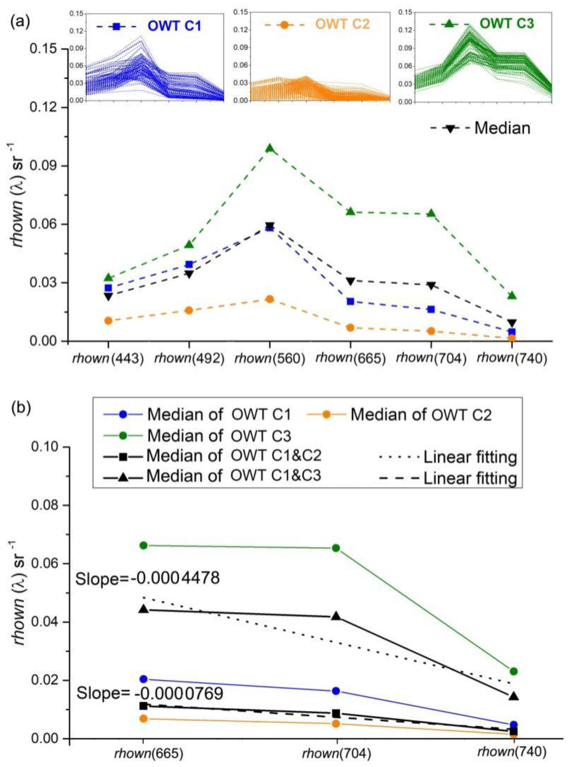
4.2. Lake Optical Water Types Clustering
4.3. BP-TURB Models
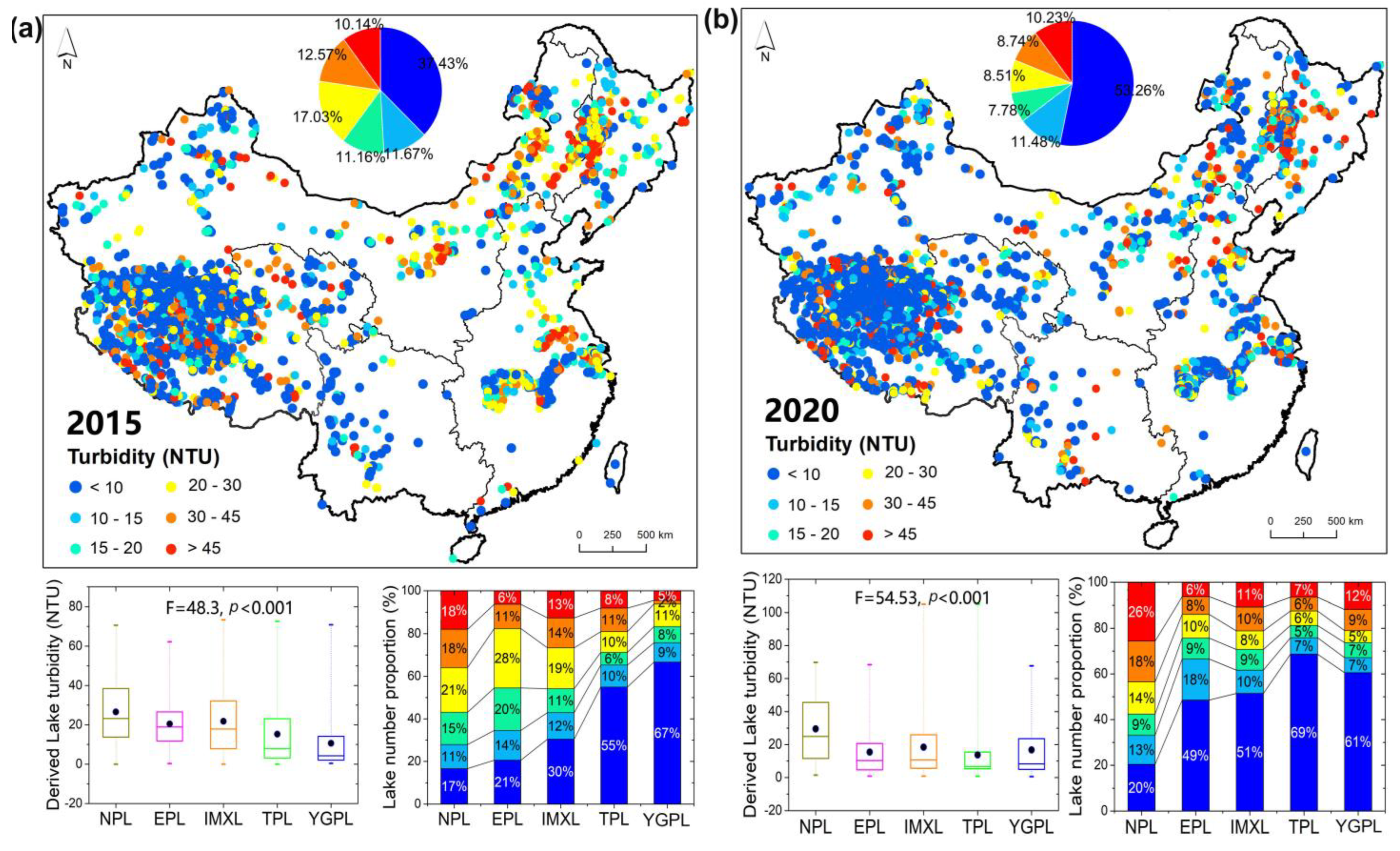
4.4. Spatial Distributions of Turbidity in 2015 and 2020
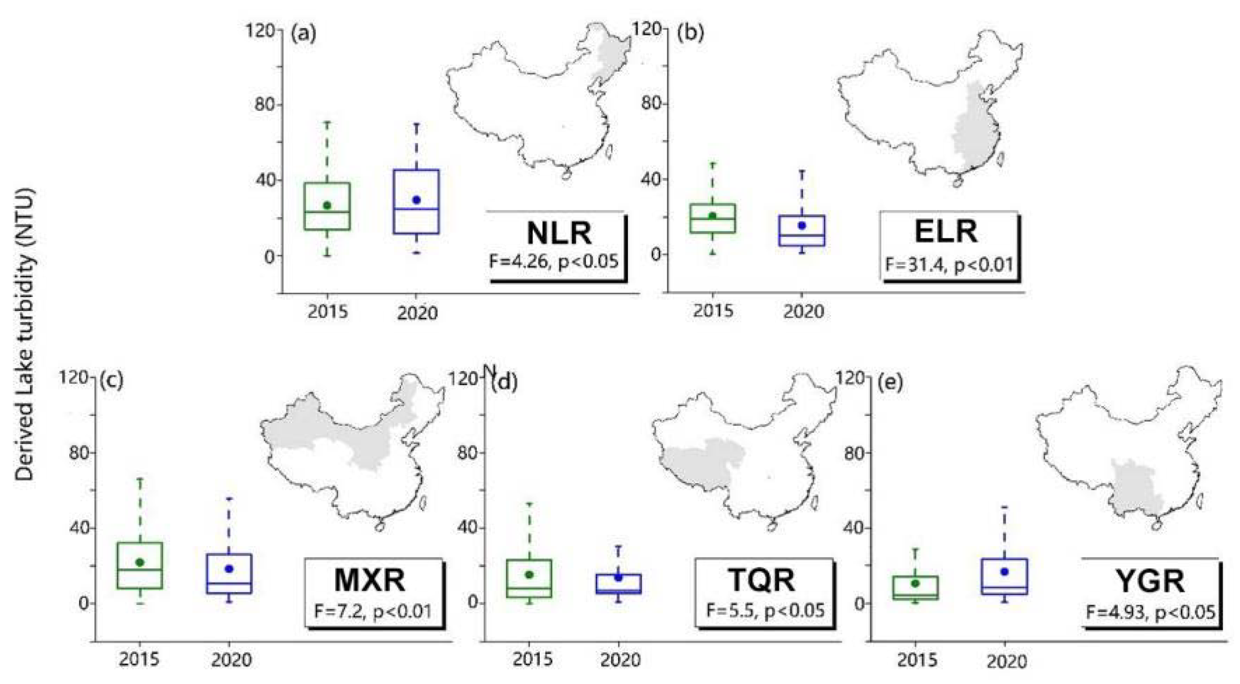
4.5. Temporal Dynamics of Lake Turbidity (>1 km2)
4.5.1. Temporal Average and Trend in Lake Turbidity
4.5.2. Interannual Changes in Turbidity
4.6. Abiotic Factors Acting on the Spatial Variations of Turbidity
5. Discussion
5.1. OWTs Clustering for Turbidity Modeling
5.2. Remotely Sensed Turbidity Models
5.3. Chinese Lake Turbidity Distributions in Five Limnetic Regions
5.4. Comparison with Past Studies, Uncertainties, Challenges, and Future Perspectives
6. Conclusions
- (1)
- The rhown(λ), consistent with in situ samples, was optimally divided into three OWTs (i.e., OWT C1, OWT C2, and OWT C3) with notable differences (ANOVA, p < 0.001) in water properties, e.g., pH, SPM, TP, SDD, aCDOM(λ), aph(λ), ad(λ), and EC.
- (2)
- The developed BP-TURB models, including BP-TURB OWT C1, BP-TURB OWT C2, and BP-TURB OWT C3, performed well with slopes close to 1 (slope > 0.82), R2 > 0.81, RMSE < 17.54, and MAE < 11.20.
- (3)
- For Chinese lakes, a larger percentage of clear lakes (53.26%) with low turbidity levels (<10 NTU) was found in 2020 than in 2015 (37.43%). The turbidity patterns were determined by lake volume, average depth, and elevation.
Supplementary Materials
Author Contributions
Funding
Data Availability Statement
Acknowledgments
Conflicts of Interest
References
- Lampert, W.; Sommer, U. Limnoecology: The Ecology of Lakes and Streams; Oxford University Press: Oxford, UK, 2007. [Google Scholar]
- Maberly, S.C.; O’Donnell, R.A.; Woolway, R.I.; Cutler, M.E.J.; Gong, M.; Jones, I.D.; Merchant, C.J.; Miller, C.A.; Politi, E.; Scott, E.M.; et al. Global lake thermal regions shift under climate change. Nat. Commun. 2020, 11, 1232. [Google Scholar] [CrossRef] [PubMed]
- Davies-Colley, R.J.; Smith, D.G. Turbidity Suspended Sediment, and Water Clarity: A Review 1. JAWRA J. Am. Water Resour. Assoc. 2001, 37, 1085–1101. [Google Scholar] [CrossRef]
- Anderson, C.W. Turbidity 6.7. In USGS National Field Manual for The Collection of Water Quality Data; US Geological Survey: Reston, VA, USA, 2005. [Google Scholar]
- Petus, C.; Chust, G.; Gohin, F.; Doxaran, D.; Froidefond, J.-M.; Sagarminaga, Y. Estimating turbidity and total suspended matter in the Adour River plume (South Bay of Biscay) using MODIS 250-m imagery. Cont. Shelf Res. 2010, 30, 379–392. [Google Scholar] [CrossRef]
- Michaud, J.P. A Citizen’s Guide to Understanding and Monitoring Lakes and Streams; Publ. #94–149; Washington State Department of Ecology, Publications Office: Olympia, WA, USA, 1991. [Google Scholar]
- Jacobsen, L.; Berg, S.; Baktoft, H.; Nilsson, P.A.; Skov, C. The effect of turbidity and prey fish density on consumption rates of piscivorous Eurasian perch Perca fluviatilis. J. Limnol. 2014, 73, 187–190. [Google Scholar] [CrossRef]
- Woolway, R.I.; Merchant, C.J. Wordlwide alteration of lake mixing regimes in response to climate change. Nat. Geosci. 2019, 12, 271–276. [Google Scholar] [CrossRef]
- Dudgeon, D.; Arthington, A.H.; Gessner MO Kawabata, Z.I.; Knowler, D.J.; Lévêque, C.; Naiman, R.J.; Prieur-Richard, A.H.; Soto, D.; Stiassny, M.L.; Sullivan, C.A. Freshwater biodiversity: Importance, threats, status and conservation challenges. Biol. Rev. 2006, 81, 163–182. [Google Scholar] [CrossRef]
- Moore, G.K. Satellite remote sensing of water turbidity/Sonde de télémesure par satellite de la turbidité de l’eau. Hydrol. Sci. J. 1980, 25, 407–421. [Google Scholar] [CrossRef]
- Ma, Y.; Song, K.; Wen, Z.; Liu, G.; Shang, Y.; Lyu, L.; Du, J.; Yang, Q.; Li, S.; Tao, H.; et al. Remote sensing of turbidity for lakes in northeast China using Sentinel-2 images with machine learning algorithms. IEEE J. Sel. Top. Appl. Earth Obs. Remote Sens. 2021, 14, 9132–9146. [Google Scholar] [CrossRef]
- Wang, Y.; Feng, L.; Liu, J.; Hou, X.; Chen, D. Changes of inundation area and water turbidity of Tonle Sap Lake: Responses to climate changes or upstream dam construction? Environ. Res. Lett. 2020, 15, 0940a1. [Google Scholar] [CrossRef]
- Toth, C.; Jóźków, G. Remote sensing platforms and sensors: A survey. ISPRS J. Photogramm. Remote Sens. 2016, 115, 22–36. [Google Scholar] [CrossRef]
- Olmanson, L.G.; Brezonik, P.L.; Bauer, M.E. Evaluation of medium to low resolution satellite imagery for regional lake water quality assessments. Water Resour. Res. 2011, 47, W09515. [Google Scholar] [CrossRef]
- Toming, K.; Kutser, T.; Laas, A.; Sepp, M.; Paavel, B.; Nõges, T. First experiences in mapping lake water quality parameters with Sentinel-2 MSI imagery. Remote Sens. 2016, 8, 640. [Google Scholar] [CrossRef]
- Li, S.; Song, K.; Wang, S.; Liu, G.; Wen, Z.; Shang, Y.; Lyu, L.; Chen, F.; Xu, S.; Tao, H.; et al. Quantification of chlorophyll-a in typical lakes across China using Sentinel-2 MSI imagery with machine learning algorithm. Sci. Total Environ. 2021, 778, 146271. [Google Scholar] [CrossRef]
- Pahlevan, N.; Chittimalli, S.K.; Balasubramanian, S.V.; Vellucci, V. Sentinel-2/Landsat-8 product consistency and implications for monitoring aquatic systems. Remote Sens. Environ. 2019, 220, 19–29. [Google Scholar] [CrossRef]
- Soomets, T.; Uudeberg, K.; Jakovels, D.; Brauns, A.; Zagars, M.; Kutser, T. Validation and comparison of water quality products in baltic lakes using sentinel-2 msi and sentinel-3 OLCI data. Sensors 2020, 20, 742. [Google Scholar] [CrossRef]
- Zhang, G.; Yao, T.; Chen, W.; Zheng, G.; Shum, C.K.; Yang, K.; Piao, S.; Sheng, Y.; Yi, S.; Li, J.; et al. Regional differences of lake evolution across China during 1960s–2015 and its natural and anthropogenic causes. Remote Sens. Environ. 2019, 221, 386–404. [Google Scholar] [CrossRef]
- Hou, X.; Feng, L.; Duan, H.; Chen, X.; Sun, D.; Shi, K. Fifteen-year monitoring of the turbidity dynamics in large lakes and reservoirs in the middle and lower basin of the Yangtze River, China. Remote Sens. Environ. 2017, 190, 107–121. [Google Scholar] [CrossRef]
- Wang, X.; Song, K.; Wen, Z.; Liu, G.; Shang, Y.; Fang, C.; Lyu, L.; Wang, Q. Quantifying Turbidity Variation for Lakes in Daqing of Northeast China Using Landsat Images From 1984 to 2018. IEEE J. Sel. Top. Appl. Earth Obs. Remote Sens. 2021, 14, 8884–8897. [Google Scholar] [CrossRef]
- Feng, L.; Hu, C.; Chen, X.; Tian, L.; Chen, L. Human induced turbidity changes in Poyang Lake between 2000 and 2010: Observations from MODIS. J. Geophys. Res. Ocean. 2012, 117, C07006. [Google Scholar] [CrossRef]
- Antoine, D.; André, J.M.; Morel, A. Oceanic primary production: 2. Estimation at global scale from satellite (coastal zone color scanner) chlorophyll. Glob. Biogeochem. Cycles 1996, 10, 57–69. [Google Scholar] [CrossRef]
- Liu, D.; Duan, H.; Loiselle, S.; Hu, C.; Zhang, G.; Li, J.; Yang, H.; Thompson, J.R.; Cao, Z.; Shen, M.; et al. Observations of water transparency in China’s lakes from space. Int. J. Appl. Earth Obs. Geoinf. 2020, 92, 102187. [Google Scholar] [CrossRef]
- Nechad, B.; Ruddick, K.G.; Park, Y. Calibration and validation of a generic multisensor algorithm for mapping of total suspended matter in turbid waters. Remote Sens. Environ. 2010, 114, 854–866. [Google Scholar] [CrossRef]
- Rodríguez-López, L.; Duran-Llacer, I.; González-Rodríguez, L.; Cardenas, R.; Urrutia, R. Retrieving water turbidity in araucanian lakes (South-central chile) based on multispectral landsat imagery. Remote Sens. 2021, 13, 3133. [Google Scholar] [CrossRef]
- Mouw, C.B.; Greb, S.; Aurin, D.; DiGiacomo, P.M.; Lee, Z.; Twardowski, M.; Binding, C.; Hu, C.; Ma, R.; Moore, T.; et al. Aquatic color radiometry remote sensing of coastal and inland waters: Challenges and recommendations for future satellite missions. Remote Sens. Environ. 2015, 160, 15–30. [Google Scholar] [CrossRef]
- Palmer, S.C.; Kutser, T.; Hunter, P.D. Remote sensing of inland waters: Challenges, progress and future directions. Remote Sens. Environ. 2015, 157, 1–8. [Google Scholar] [CrossRef]
- Spyrakos, E.; O’Donnell, R.; Hunter, P.D.; Miller, C.; Scott, M.; Simis, S.G.H.; Neil, C.; Barbosa, C.C.F.; Binding, C.E.; Bradt, S.; et al. Optical types of inland and coastal waters. Limnol. Oceanogr. 2018, 63, 846–870. [Google Scholar] [CrossRef]
- Neil, C.; Spyrakos, E.; Hunter, P.D.; Tyler, A.N. A global approach for chlorophyll-a retrieval across optically complex inland waters based on optical water types. Remote Sens. Environ. 2019, 229, 159–178. [Google Scholar] [CrossRef]
- Song, K.; Wen, Z.; Jacinthe, P.A.; Zhao, Y.; Du, J. Dissolved carbon and CDOM in lake ice and underlying waters along a salinity gradient in shallow lakes of Northeast China. J. Hydrol. 2019, 571, 545–558. [Google Scholar] [CrossRef]
- Song, K.; Wang, Q.; Liu, G.; Jacinthe, P.-A.; Li, S.; Tao, H.; Du, Y.; Wen, Z.; Guo, W.; Wang, Z.; et al. A unified model for high resolution mapping of global lake (>1 ha) clarity using Landsat imagery data. Sci. Total Environ. 2022, 810, 151188. [Google Scholar] [CrossRef]
- Li, S.; Chen, F.; Song, K.; Liu, G.; Tao, H.; Xu, S.; Wang, X.; Mu, G. Mapping the trophic state index of eastern lakes in China using an empirical model and Sentinel-2 imagery data. J. Hydrol. 2022, 608, 127613. [Google Scholar] [CrossRef]
- Wang, S.M.; Dou, H.S. Lakes in China; Science press: Beijing, China, 1998.
- APHA. Standard Methods for the Examination of Water and Wastewater, 20th ed.; American Public Health Association: Washington, DC, USA; American Water Works Association: Austin, TX, USA; Water Environment Federation: Alexandria, VA, USA, 1998. [Google Scholar]
- Bricaud, A.; Babin, M.; Morel, A.; Claustre, H. Variability in the chlorophyll-specific absorption coefficients of natural phytoplankton: Analysis and parameterization. J. Geophys. Res. Ocean. 1995, 100, 13321–13332. [Google Scholar] [CrossRef]
- Warren, M.A.; Simis, S.G.; Selmes, N. Complementary water quality observations from high and medium resolution Sentinel sensors by aligning chlorophyll-a and turbidity algorithms. Remote Sens. Environ. 2021, 265, 112651. [Google Scholar] [CrossRef]
- Sass, G.Z.; Creed, I.F.; Bayley, S.E.; Devito, K.J. Understanding variation in trophic status of lakes on the Boreal Plain: A 20 year retrospective using Landsat TM imagery. Remote Sens. Environ. 2007, 109, 127–141. [Google Scholar] [CrossRef]
- Wickel, B.A.; Lehner, B.; Sindorf, N. HydroSHEDS: A Global Comprehensive Hydrographic Dataset. In Proceedings of the AGU Fall Meeting Abstracts, San Francisco, CA, USA, 10–14 September 2007; American Geophysical Union: Washington, DC, USA, 2007; Volume 2007, p. H11H–05. [Google Scholar]
- Messager, M.L.; Lehner, B.; Grill, G.; Nedeva, I.; Schmitt, O. Estimating the volume and age of water stored in global lakes using a geo-statistical approach. Nat. Commun. 2016, 7, 1–11. [Google Scholar] [CrossRef]
- Ruddick, K.; Vanhellemont, Q.; Yan, J.; Neukermans, G.; Wei, G.; Shang, S. Variability of suspended particulate matter in the Bohai Sea from the geostationary Ocean Color Imager (GOCI). Ocean. Sci. J. 2012, 47, 331–345. [Google Scholar] [CrossRef]
- Ouma, Y.O.; Noor, K.; Herbert, K. Modelling reservoir chlorophyll-a, TSS, and turbidity using Sentinel-2A MSI and Landsat-8 OLI satellite sensors with empirical multivariate regression. J. Sens. 2020, 2020, 1–21. [Google Scholar] [CrossRef]
- Feng, L.; Hou, X.; Zheng, Y. Monitoring and understanding the water transparency changes of fifty large lakes on the Yangtze Plain based on long-term MODIS observations. Remote Sens. Environ. 2019, 221, 675–686. [Google Scholar] [CrossRef]
- Moore, T.S.; Dowell, M.D.; Bradt, S.; Verdu, A.R. An optical water type framework for selecting and blending retrievals from bio-optical algorithms in lakes and coastal waters. Remote Sens. Environ. 2014, 143, 97–111. [Google Scholar] [CrossRef]
- Page, B.P.; Olmanson, L.G.; Mishra, D.R. A harmonized image processing workflow using Sentinel-2/MSI and Landsat-8/OLI for mapping water clarity in optically variable lake systems. Remote Sens. Environ. 2019, 231, 111284. [Google Scholar] [CrossRef]
- Matsushita, B.; Yang, W.; Yu, G.; Oyama, Y.; Yoshimura, K.; Fukushima, T. A hybrid algorithm for estimating the chlorophyll-a concentration across different trophic states in Asian inland waters. ISPRS J. Photogramm. Remote Sens. 2015, 102, 28–37. [Google Scholar] [CrossRef]
- Smith, M.E.; Lain, L.R.; Bernard, S. An optimized chlorophyll a switching algorithm for MERIS and OLCI in phytoplankton-dominated waters. Remote Sens. Environ. 2018, 215, 217–227. [Google Scholar] [CrossRef]
- Babin, M.; Stramski, D.; Ferrari, G.M.; Claustre, H.; Bricaud, A.; Obolensky, G.; Hoepffner, N. Variations in the light absorption coefficients of phytoplankton, nonalgal particles, and dissolved organic matter in coastal waters around Europe. J. Geophys. Res. Ocean. 2003, 108, 3211. [Google Scholar] [CrossRef]
- Song, K.; Liu, G.; Wang, Q.; Wen, Z.; Lyu, L.; Du, Y.; Sha, L.; Fang, C. Quantification of lake clarity in China using Landsat OLI imagery data. Remote Sens. Environ. 2020, 243, 111800. [Google Scholar] [CrossRef]
- IOCCG. Earth Observations in Support of Global Water Quality Monitoring; IOCCG Report; Greb, S., Dekker, A., Binding, C., Eds.; International Ocean Colour Coordinating Group (IOCCG): Dartmouth, NS, Canada, 2018. [Google Scholar]
- Kutser, T.; Verpoorter, C.; Paavel, B.; Tranvik, L.J. Estimating lake carbon fractions from remote sensing data. Remote Sens. Environ. 2015, 157, 138–146. [Google Scholar] [CrossRef]
- Mi, H.; Fagherazzi, S.; Qiao, G.; Hong, Y.; Fichot, C.G. Climate change leads to a doubling of turbidity in a rapidly expanding Tibetan lake. Sci. Total Environ. 2019, 688, 952–959. [Google Scholar] [CrossRef]
- Wang, C.; Wei, Z.; Zhao, Y.; Bai, L.; Jiang, H.; Xu, H.; Xu, Y. Resuspension and settlement characteristics of lake sediments amended by phosphorus inactivating materials: Implications for environmental remediation. J. Environ. Manag. 2022, 302, 113892. [Google Scholar] [CrossRef]
- Kiselev, V.; Bulgarelli, B.; Heege, T. Sensor independent adjacency correction algorithm for coastal and inland water systems. Remote Sens. Environ. 2015, 157, 85–95. [Google Scholar] [CrossRef]
- Ma, R.; Duan, H.; Liu, Q.; Loiselle, S.A. Approximate bottom contribution to remote sensing reflectance in Taihu Lake, China. J. Great Lakes Res. 2011, 37, 18–25. [Google Scholar] [CrossRef]
- Cleveland, J.; Weidemann, A. Quantifying absorption by aquatic particles: A multiple scattering correction for glass-fiber filters. Limnol. Oceanogr. 2013, 38, 1321–1327. [Google Scholar] [CrossRef]
- Wang, X.; Siegert, F.; Zhou, A.; Franke, J. Glacier and glacial lake changes and their relationship in the context of climate change, Central Tibetan Plateau 1972–2010. Global Planet Chang. 2013, 111, 246–257. [Google Scholar] [CrossRef]
- Jeffrey, S.W.; Humphrey, G.F. New Spectrophotometric Equations for Determing Chlorophyll a, b, c1 and c2 in Higher Plants, Algae and Natural Phycoplankton. J. Plant Physiol. 1975, 167, 191–194. [Google Scholar]
- Babin, M.; Stramski, D.; Ferrari, G. Variations in the light absorption coefficients of phytoplankton, nonalgal particles, and dissolved organic mat-ter in coastal waters around Europe. J. Geophys Res. Oceans 2003, 108. [Google Scholar]


| Parameters | N | Avg. | SD. | Min. | Max |
|---|---|---|---|---|---|
| Turbidity (NTU) + | 484 | 39.19 | 31.12 | 0 | 282.74 |
| pH | 431 | 8.51 | 1.04 | 6.86 | 13.05 |
| EC (µS cm−1) | 431 | 3252.3 | 6739.31 | 0.17 | 33,453.10 |
| SDD (m) | 431 | 1.60 | 1.50 | 0.17 | 9.47 |
| SPM (mg L−1) | 484 | 15.77 | 21.00 | 0.24 | 147.50 |
| Chl-a (µg L−1) | 431 | 7.56 | 11.28 | 0.13 | 100.22 |
| TP (mg L−1) | 431 | 0.16 | 0.42 | 0.003 | 2.17 |
| ap(443) (m−1) | 431 | 1.41 | 1.76 | 0.01 | 8.06 |
| aph(443) (m−1) | 431 | 0.48 | 0.72 | 0 | 5.33 |
| ad(443) (m−1) | 431 | 0.93 | 1.43 | 0 | 6.96 |
| aCDOM(443) (m−1) | 431 | 0.54 | 0.43 | 0 | 1.89 |
| Models | Input Band Combinations or Model | Datasets | N | Slopes * | R2 | Errors |
|---|---|---|---|---|---|---|
| BP-TURB OWT C1 | Input: rhown (443, 490, 560, 665, 704 and 740) | Cal- | 76 | 0.84 | 0.87 | RMSE = 4.01; MAE = 2.99 |
| Val- | 39 | 0.83 | 0.88 | RMSE = 4.42; MAE = 3.00 | ||
| BP-TURB OWT C2 | Input: rhown (443, 490, 560, 665, 704 and 740); rhown (665 × 704 × 740/443); rhown(560 × 704 × 665/443); rhown(704 × 740/490); rhown(704 + 740/443); rhown(704+740/560); rhown(665 + 704 + 490/443); rhown(704 × 740) | Cal- | 163 | 0.83 | 0.81 | RMSE = 3.24; MAE = 2.51 |
| Val- | 82 | 0.82 | 0.81 | RMSE = 3.67; MAE = 2.91 | ||
| BP-TURB OWT C3 | Input: rhown (443, 490, 560, 665, 704 and 740); rhown(704 × 740/490); rhown(665 × 704/490); rhown(704 × 740/665); rhown(560 × 740/443); rhown(490 × 665 × 704/443); rhown(665 × 704 × 740/443); rhown(560 × 740/443); rhown(665 × 704/443); rhown(704 × 740/443); rhown(490 × 704 × 740/443); rhown(490 × 740/443); rhown(704 × 740) | Cal- | 131 | 0.87 | 0.79 | RMSE = 27.74; MAE = 20.92 |
| Val- | 64 | 0.89 | 0.81 | RMSE = 17.54; MAE = 11.20 | ||
| Multiple Linear regressions | Input: rhown(740) Cal-:Tur =2059.14 × rhown(740) + 0.669 Val-:Tur estimated = 0.63 × Tur measured + 7.18 | Cal- | 370 | - | 0.56 | RMSE = 14.96; MAE = 8.02 |
| Val- | 185 | 0.63 | 0.53 | RMSE = 15.12, MAE = 8.12 | ||
| Input: rhown(709), rhown(740) Cal-:Tur = 6867.67 × rhown(740)–1752.26 × rhown(709) + 3.96 Val-:Tur estimated = 0.64 × Tur measured + 6.87 | Cal- | 370 | - | 0.55 | RMSE = 27.20; MAE = 17.36 | |
| Val- | 185 | 0.64 | 0.55 | RMSE = 48.60; MAE = 30.11, |
Disclaimer/Publisher’s Note: The statements, opinions and data contained in all publications are solely those of the individual author(s) and contributor(s) and not of MDPI and/or the editor(s). MDPI and/or the editor(s) disclaim responsibility for any injury to people or property resulting from any ideas, methods, instructions or products referred to in the content. |
© 2023 by the authors. Licensee MDPI, Basel, Switzerland. This article is an open access article distributed under the terms and conditions of the Creative Commons Attribution (CC BY) license (https://creativecommons.org/licenses/by/4.0/).
Share and Cite
Li, S.; Kutser, T.; Song, K.; Liu, G.; Li, Y. Lake Turbidity Mapping Using an OWTs-bp Based Framework and Sentinel-2 Imagery. Remote Sens. 2023, 15, 2489. https://doi.org/10.3390/rs15102489
Li S, Kutser T, Song K, Liu G, Li Y. Lake Turbidity Mapping Using an OWTs-bp Based Framework and Sentinel-2 Imagery. Remote Sensing. 2023; 15(10):2489. https://doi.org/10.3390/rs15102489
Chicago/Turabian StyleLi, Sijia, Tiit Kutser, Kaishan Song, Ge Liu, and Yong Li. 2023. "Lake Turbidity Mapping Using an OWTs-bp Based Framework and Sentinel-2 Imagery" Remote Sensing 15, no. 10: 2489. https://doi.org/10.3390/rs15102489
APA StyleLi, S., Kutser, T., Song, K., Liu, G., & Li, Y. (2023). Lake Turbidity Mapping Using an OWTs-bp Based Framework and Sentinel-2 Imagery. Remote Sensing, 15(10), 2489. https://doi.org/10.3390/rs15102489