Evaluation of Partitioned Evaporation and Transpiration Estimates within the DisALEXI Modeling Framework over Irrigated Crops in California

Abstract

Accurate characterization of evapotranspiration (ET) is imperative in water-limited cropping systems such as California vineyards and almond orchards. Satellite-based ET modeling techniques, including the atmosphere–land exchange inverse model (ALEXI) and associated flux disaggregation technique (DisALEXI), have proven reliable in determining field scale ET. However, validation efforts typically focus on ET and omit an evaluation of partitioned evaporation (E) and transpiration (T). ALEXI/DisALEXI is based on the two-source energy balance (TSEB) model, making it uniquely qualified to derive E and T individually. The current study evaluated E and T estimates derived using two formulations of DisALEXI; one based on Priestley-Taylor (DisALEXI-PT) and the other on Penman-Monteith (DisALEXI-PM). The modeled values were validated against partitioned fluxes derived from the conditional eddy covariance (CEC) approach using EC flux towers in three wine grape vineyards and three almond orchards for the year 2021. Modeled estimates were derived using Landsat 8 Collection 2 thermal infrared and surface reflectance imagery as well as Harmonized Landsat and Sentinel-2 surface reflectance datasets as input into DisALEXI. The results indicated that the modeled total ET fluxes were similar between the two methods, but the partitioned values diverged, with DisALEXI-PT overestimating E and slightly underestimating T when compared to CEC estimates. Conversely, DisALEXI-PM agreed better with CEC-derived E and overestimated T estimates under non-advective conditions. Compared to one another, DisALEXI-PM estimated canopy temperatures ~5 °C cooler and soil temperatures ~5 °C warmer than DisALEXI-PT, causing differences in E and T of −2.6 mm day⁻¹ and +2.6 mm day⁻¹, respectively. The evaluation of the iterative process required for DisALEXI indicates DisALEXI-PM ET values converge on ALEXI ET with proportionate adjustments to E and T, while DisALEXI-PT convergence is driven by adjustments to E. The analysis presented here can potentially drive improvements in the modeling framework to provide specific soil and canopy consumptive water use information in unique canopy structures, allowing for improved irrigation and water use efficiencies in these water-limited systems.

1. Introduction

Acquiring accurate measurements of crop consumptive water use in the form of evapotranspiration (ET) is increasingly important as demands for water resources drastically shift under a changing climate. This acquisition is particularly critical in the Central Valley of California, where competition for diminishing water resources is increasing due to prolonged periods of severe drought, population growth, and increasing demands from municipalities and industry [1]. Such are the demands that the state enacted the Sustainable Groundwater Management Act (SGMA), an effort to monitor and regulate the over-pumping of vulnerable groundwater basins.

Considering these regulations, California-based commodity groups continue to have a vested interest in the sustainability of agriculture in the state, which is valued at USD 50 billion per year [2,3] and produces more than 400 different commodities. This interest has produced partnerships with federal and state agencies and universities to promote sustainable practices through the research and development of emerging state-of-the-art technologies focused on promoting water use efficiency. Two such projects include the Grape Remote Sensing Atmospheric Profile Evapotranspiration eXperiment (GRAPEX; [4]) and the Tree crop Remote sensing of Evapotranspiration eXperiment (T-REX), where the priority is to improve irrigation efficiencies through satellite-derived ET estimates for wine grapes and almond orchards, respectively. GRAPEX began in 2013 and continues with nine vineyards being monitored with micrometeorological instrumentation located throughout the Central Valley and Sonoma County, California. T-REX began in the spring of 2021 and continues to support the monitoring of three almond orchards located near Sacramento and Fresno, California.

Much has been learned during the GRAPEX project, which includes ground-based micrometeorological/biophysical-focused work [4,5,6,7,8], the utilization of remotely piloted aerial vehicles (RPAVs) for an improved understanding of spatial dynamics within vineyards [9,10,11,12,13,14], and the evaluation of satellite-based ET estimates, both retrospectively [15,16,17,18] and in real-time [19], to promote ingestion into irrigation management dashboards. Similar work is currently underway in the T-REX project. Although work related to these projects has advanced our understanding of specialty crop dynamics as it relates to water use, questions remain. One of particular interest is the partitioning of ET, used as a measure of consumptive water use, into individual contributions of evaporation (E) and transpiration (T) in these vineyard/orchard systems, which are represented by distinct inter-row (denoted by cover crop or bare soil depending on management practice and time of year) and row (crop canopy). In water-limited regions such as California, some irrigation strategies will likely focus on reducing water loss from E rather than T since vegetation T is linked to crop biomass production [20,21,22].

Many ET partitioning techniques exist (detailed review provided in [23]), with recent advancements developed to curb laborious measurements, expensive sensors, and the need for a priori site knowledge [24,25,26]. Despite advancements, these approaches cannot be inferred or spatially distributed across large landscapes. Such a solution requires the utilization of remote sensing, whether from RPAVs or satellite imagery, and an approach that explicitly accounts for soil (E) and canopy (T) contributions to ET. The two-source energy balance (TSEB) model [27] offers these capabilities by partitioning a thermal infrared (TIR) signal into canopy and soil temperatures and solving the surface-energy budget for the soil, vegetation, and combined systems associated with a mixed pixel. TSEB has been applied across many surfaces [28,29,30,31,32,33,34,35], including vineyards, with good fidelity [9,10,12,34,36,37]. However, these studies evaluated TSEB in terms of total (soil + canopy) ET rather than the individual contributions of E and T.

Individual flux evaluation within TSEB began with [28], where it was found that estimates of total heat fluxes were acceptable, but the partitioning of available energy between soil and canopy fluxes was not physically realistic. These findings led to modifications within TSEB to improve partitioning, including the recommendation to increase the Priestley-Taylor parameter over sparse canopy cover where advective heat sources from adjacent hot bare soil surfaces can contribute significantly as an additional energy source [28]. Reference [38] offered an evaluation of TSEB based on calculated versus measured E, T, and ET. The results suggest that replacing the Priestley-Taylor (PT) formulation [39] with Penman-Monteith (PM) provides a more accurate partitioning of E and T. This is because the PM formulation more directly accounts for vapor pressure deficit (VPD), whereas the PT formulation assumes the influence of VPD is accounted for in the fixed PT parameter. A consequent study performed by [40], which occurred at a fully irrigated cotton field indicative of highly advective conditions, reported improved TSEB E and T estimation when applying PM in lieu of PT. Similar results were found in other PT-based ET studies, when the PT parameter is calculated as an empirical function based on VPD (e.g., [32,41,42]) or when it is increased when VPD exceeds a predefined value, such as in the initial [28] study mentioned above. Each imitates the VPD (i.e., aerodynamic) term in PM, proving its importance and offering an explanation as to why PM outperforms PT within the context of TSEB in advective systems.

Recent TSEB-based partitioning studies have focused on vineyards as part of the GRAPEX project [36,43,44]. Reference [36] applied TSEB over two Pinot Noir vineyards in the Central Valley of California and compared modeled T/ET ratios to observations derived using the correlation-based flux partitioning method [45,46,47]. The results indicate TSEB E and T estimates yield relative differences with flux tower measurements of less than 15%. However, the results are heavily dependent on the time of year; e.g., TSEB overestimates T/ET during winter and spring but underestimates during the growing season [36]. Reference [44] attempted to improve modeled partitioned fluxes in vineyard systems by proposing a three-source energy balance (3SEB) model, accommodating an additional vegetation source within TSEB. The results were promising, with modeled T correlating better than TSEB with observations derived from an eddy covariance-based partitioning approach (R > 0.76). Despite improvements, the results still indicate a slight underestimation of T/ET, particularly when the cover crop between vine rows is absent [44]. Perennial natural ecosystems (trees) and agroecosystems (vineyards) have a strong physiological and stomatal control of ET under conditions of high VPD [48,49,50,51]. As described above, the PT initialization in TSEB or 3SEB may not fully capture these effects. As demonstrated in [38,40], alternative initialization formulations in TSEB, such as PM, which better account for VPD, may be required to accurately capture T/ET values in advective systems and agroecosystems characteristic of having bare inter-rows.

Reference [43] offers an evaluation of advective conditions within the context of TSEB and vineyards by exploring the effects different levels of advection have on derived T/ET estimates from different modified versions of TSEB over a vineyard in the Central Valley of California. The results suggest the performance of the original PT-based TSEB is satisfactory in all but the most extreme advective conditions. They also found a transpiration algorithm based on Shuttleworth-Wallace, which includes a canopy resistance formula that relates maximum stomata conductance to VPD and performs well under all conditions [43]. An evaluation of a PM-based TSEB (similar to [38]) showed improvements only under the more extreme advective conditions and over-estimated T/ET under the remaining conditions.

Although work related to TSEB-based E and T partitioning has led to many insights, most notably the relationship between canopy transpiration (i.e., T) and VPD, it has relied on ground-based thermal infrared measurements as an input and has only been evaluated at individual sites. Such approaches omit the capable spatial component of TSEB through the utilization of satellite-derived thermal infrared imagery. Spatially distributed ET estimates from TSEB can be produced using the Atmosphere–Land Exchange Inverse model (ALEXI; [52,53,54]) and the associated disaggregation technique (DisALEXI; [55,56]). As with TSEB, the combined ALEXI/DisALEXI modeling framework has been applied in vineyards as part of the GRAPEX project [15,16,17,19,57,58,59,60]. DisALEXI is also implemented within the OpenET framework on Google Earth Engine, which supplies ET information across 17 western U.S. states in support of water management and decision making [61]. Although ALEXI/DisALEXI produces reliable ET estimates in vineyard settings, there has yet to be a thorough analysis of the individual contributions of E and T to the total ET flux in the context of DisALEXI. Additionally, given the operational capabilities of ALEXI/DisALEXI (OpenET, irrigation decision making) and the increasing importance of individual flux contributions in water-limited agricultural systems requiring irrigation–such as vineyards and almonds orchards—the evaluation of E and T partitioning will be necessary for developing robust applications.

This study evaluates the partitioning of E and T within the context of the ALEXI/DisALEXI modeling framework. Analysis was performed over three wine grape vineyards (GRAPEX sites) and three almond orchards (T-REX sites) for the year 2021, using tower measurements of total ET (as defined in [7]) as well as individual E and T estimates that were calculated using the conditional eddy covariance (CEC) approach as described in [26]). We evaluate the original DisALEXI approach based on the Priestley-Taylor formulation of TSEB (DisALEXI-PT) and the iterative convergence process with ALEXI for irrigated vineyards/orchards in the advective climate characterizing the GRAPEX and T-REX sites. We also evaluate a DisALEXI approach based on the Penman-Monteith formulation (DisALEXI-PM), as first suggested by [38]. Due to the advective nature of the study sites and their characteristically barren inter-rows during the growing season, we hypothesize that shifting to a Penman-Monteith-based approach will improve model partitioned estimates of E and T. When applied operationally, the model output will give growers more specific consumptive water use information, subsequently allowing for improved irrigation and water use efficiencies in these valuable water-limited agricultural systems.

2. Materials and Methods

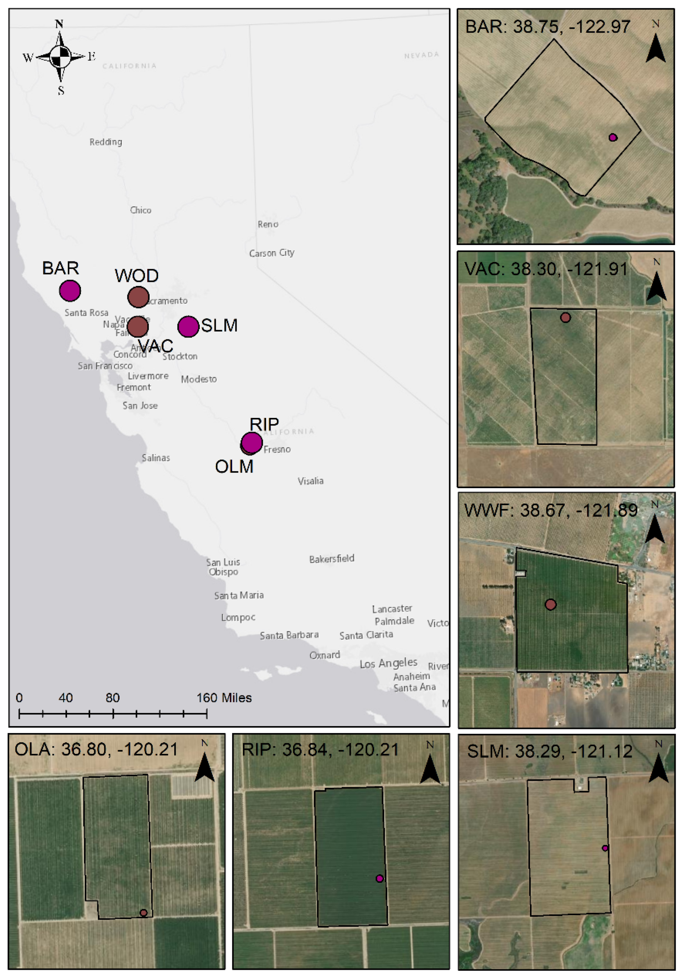
2.1. Study Domain

The study domain encompasses four separate regions across California and includes three individual wine grape vineyards being monitored as part of the USDA-ARS Grape Remote sensing Atmospheric Profile and Evapotranspiration eXperiment (GRAPEX) [4] and three individual almond orchards being monitored as part of the USDA-ARS Tree crop Remote sensing of Evapotranspiration eXperiment (T-REX) (Figure 1). Vineyards include BAR (Sonoma County near Cloverdale, CA, USA), SLM (Sacramento County near Galt, CA, USA), and RIP (Madera County near Madera, CA, USA). BAR is a 10-ha plot composed of Cabernet Sauvignon grapes trained on a split trellis and drip irrigated. Vines were planted in 2010 with 1.8 m vine spacing and 3.35 m row spacing and have a southwest–northeast row orientation. SLM is a 35-ha plot composed of Cabernet Sauvignon grapes (regrafted in the winter of 2020) trained on quadrilateral cordons with 3.35 m row spacing, 1.5 m vine spacing, west-to-east row orientation, and drip irrigation. RIP is a 31-ha block composed of Chardonnay grapes planted in 2009 and trained on a double vertical trellis with 1.83 m vine spacing and 2.74 m row spacing, west-to-east row orientation, and drip irrigation.

Almond orchards include VAC (Solano County near Vacaville, CA), WWF (Yolo County near Woodland, CA, USA), and OLA (Madera County near Madera, CA). VAC is a 70 ha seventh-leaf orchard with 100% Independence variety and a southwest-to-northeast row orientation with drip irrigation. WWF is a 60 ha ninth-leaf orchard with 50% Nonpareil, and 17% Butte, Monterey, and Carmel varieties, north–south row orientation, and micro-sprinkler irrigation installed. OLA is a 20 ha eighth leaf orchard with 50% Nonpareil, 37% Wood Colony, and 13% Supareil, north–south row orientation, and two-line drip irrigation.

All vineyard sites have a cover crop present during the winter season. Once conditions become dry in the early summer, the cover crop is either left to senesce or removed via mowing so that water is used exclusively by vines. The northernmost site, BAR, typically has more cover crop biomass that also remains longer into the growing season in comparison with the other two vineyards. This is due to greater precipitation and higher quality grape grown at the site, which requires a cover crop to regulate soil water availability. Almond orchards OLA and VAC have native vegetation that grows in between rows that is also present during the winter season before either being mowed or allowed to senesce during the early summer months. WWF has a cover crop consisting of a seeded mix of legumes and grasses, which is present from winter through spring and then mowed after senescence.

2.2. Field Measurements

Micrometeorological and biophysical data collected at each location as part of GRAPEX and T-REX are used to evaluate, validate, and refine ET estimates, detect crop stress, and monitor biomass development and root zone soil water availability. All sites are equipped with similar instrumentation, with measurements including surface energy balance flux estimates, turbulence and mean profile measurements of wind, temperature, and water vapor, as well as periodic ground-based biophysical measurements such as leaf-water potential, leaf area index (LAI), and gas exchange.

Eddy covariance systems at the GRAPEX sites include a Campbell Scientific, Inc. integrated CO₂ and H₂O open-path gas analyzer and a three-dimensional ultrasonic anemometer collecting data at 20 Hz producing 30 min flux averages. Radiation is monitored via an NR01 four-component radiometer (Hukseflux, Delft, the Netherlands), and humidity and temperature via an EE08 probe (E+E Elektronik, Engerwitzdorf, Austria) in a TS120 fan-aspirated shield (Apogee Instruments Inc., Logan, UT, USA). Ground heat flux is estimated through an array of soil heat flux plates (HFT-3, Radiation Energy Balance Systems, Bellevue, Washington) buried at a depth of roughly 8 cm, Hydraprobe soil moisture sensors (Stevens Water Monitoring Systems, Inc., Portland, OR, USA), and soil thermocouples for estimating heat storage above the plates (see [4,6] for details of the eddy covariance and soil heat flux measurements). The eddy covariance flux systems at the T-REX sites include a similar instrumental setup with the exception of the radiation measurements monitored using a CNR4 net radiometer (Kipp and Zonen, Delft, Netherlands).

In order to further provide partitioned (separation of E and T) flux validation, we utilize a novel method based on quadrant analysis of high-frequency EC data, referred to as the conditional eddy covariance (CEC) approach [26]. The CEC approach is based on the similarity between stomatal (transpiration and photosynthesis) and non-stomatal (evaporation and respiration) pairs of component fluxes and works by combining measurements of high-frequency carbon dioxide and water vapor EC data to find all four component fluxes (transpiration, photosynthesis, evaporation, respiration) simultaneously. The CEC method is a simpler technique in comparison to other partitioning approaches (such as the modified relaxed eddy accumulation; MREA, flux-variance similarity; FVS) but circumvents the need to estimate water use efficiency (WUE) and gross primary product (GPP) as inputs. The approach has been applied in various systems, including forest, grassland, and vineyard sites [26]. Although the results were promising, particularly given the simplified approach, application within a vineyard site demonstrated some uncertainty worth mentioning. Most notable is the EC measurement height relative to the canopy height, where [26] suggests measurements be obtained as close as possible to the top of the canopy so air parcels emanating from the soil surface and canopy are not completely mixed. The EC tower height for the T-REX almond sites is roughly 5 m above the canopy, whereas the included GRAPEX vineyard sites are about 2.0 to 2.5 m above the canopy. Heights were chosen to include fetch and footprint requirements so ET observations could provide validation to remotely sensed values. Although the distance from the canopy is not ideal, we assume the CEC technique gives reasonable partitioning estimates but acknowledge potential deficiencies in the values.

To conduct a reliable and consistent comparison between daily observed measurements and modeled flux estimates, which assume closure on a daily scale, we use a closure approach offered in [7]. Specifically, nine separate EC flux energy balance closure approaches are used to derive an ensemble daily closed ET estimate at each tower location as the mean of nine daily closed ET estimates. This method effectively reduces spurious outliers potentially related to hysteresis, advection, or heat storage by equally weighting measurement’s reliability of the available energy (net radiation minus soil heat flux density) and eddy covariance sensible (H) and latent (λE) heat flux density components [7]. The CEC method applied here has been corrected for closure by distributing the difference between closed (via [7]) and unclosed ET by the fraction of E and T to total ET.

Modeled flux estimates were extracted and averaged over a 3 × 3 pixel area (90 × 90 m) shifted in the direction of the mean incoming wind to approximate the typical tower upwind fetch/flux footprint. Additional care was taken for sites located near field boundaries (VAC, OLA, RIP, SLM), making sure representative pixels did not overlay the adjacent road. We refer the reader to [7] and [26] for additional details pertaining to observations used for validation in the current study.

2.3. Satellite-Based ET Modeling Framework

2.3.1. TSEB-PT

The two-source energy balance (TSEB) model was first described in [27], with improvements presented in [28]. The TSEB model partitions surface temperature into soil and vegetation canopy components using a local vegetation cover fraction (f_c) estimated from retrievals of leaf area index (LAI) and a clumping factor dependent on vegetation class (Ω; [30]) according to Equation (1).

$${\mathrm{T}}_{\mathrm{r}}={\mathrm{f}}_{\mathrm{c}}{\mathrm{T}}_{\mathrm{c}}+\left(1-{\mathrm{f}}_{\mathrm{c}}\right){\mathrm{T}}_{\mathrm{s}},$$

(1)

Initial temperature components are then used to initiate a temperature gradient-resistance system of equations designed to solve the surface-energy budget for the soil and vegetation components (Equation (2)).

$$\left({\mathrm{Rn}}_{\mathrm{s}}+{\mathrm{Rn}}_{\mathrm{c}}\right)-\mathrm{G}=\left({\mathrm{H}}_{\mathrm{s}}+{\mathrm{H}}_{\mathrm{c}}\right)+\left({\mathsf{\lambda }\mathrm{E}}_{\mathrm{s}}+{\mathsf{\lambda }\mathrm{E}}_{\mathrm{c}}\right),$$

(2)

In the above energy balance equation, R_n is the net radiation (W m⁻²), H is the sensible heat flux (W m⁻²), G is the soil heat flux (W m⁻²), and λE is the latent heat flux (W m⁻²). Subscripts ‘s’ and ‘c’ represent fluxes associated with the soil and canopy components of the pixel, respectively. The soil and canopy components of R_n are estimated according to [62], and G is derived from a phase difference equation described by [63]. Following [27], we calculate H_s and H_c directly and λE_s as the residual (details forthcoming). However, in order to do so, an initial estimate of λE_c is obtained using the Priestley-Taylor approach [39]:

$${\mathsf{\lambda }\mathrm{E}}_{\mathrm{c}\_\mathrm{PT}}={ \mathsf{\alpha }\mathrm{f}}_{\mathrm{g}}\frac{\mathsf{\Delta }}{\mathsf{\Delta }+\mathsf{\gamma }}\left({\mathrm{Rn}}_{\mathrm{c}}\right),$$

(3)

where f_g is the fraction of green vegetation (set as 1.0), α is the Priestley-Taylor parameter (α~1.3), Δ is the slope of the saturation vapor pressure–temperature curve, γ is the psychrometric constant, and R_nc is the divergence of net radiation in the canopy calculated as an initial estimate following [27]. Canopy and soil components of sensible heat flux are calculated assuming a series network as:

$${\mathrm{H}}_{\mathrm{s}}={ \mathsf{\rho }\mathrm{C}}_{\mathrm{p}}\ast \left(\frac{{\mathrm{T}}_{\mathrm{s}}-{\mathrm{T}}_{\mathrm{ac}}}{{\mathrm{r}}_{\mathrm{s}}}\right),$$

(4)

$${\mathrm{H}}_{\mathrm{c}}={ \mathsf{\rho }\mathrm{C}}_{\mathrm{p}}\ast \left(\frac{{\mathrm{T}}_{\mathrm{c}}-{\mathrm{T}}_{\mathrm{ac}}}{{\mathrm{r}}_{\mathrm{x}}}\right),$$

(5)

where ρC_p is the volumetric heat capacity of the air, T_ac is the air temperature within the air-canopy layer, r_s is the resistance to transport heat between the soil surface and a height representing the canopy, and r_x is the total boundary layer resistance of the complete canopy of leaves. Initial T_c values are estimated using a form of the Priestley-Taylor equation (Equation (6)), whereas initial T_s values are estimated as the residual to Equation (1).

$${\mathrm{T}}_{\mathrm{c}1}={\mathrm{T}}_{\mathrm{a}}+\frac{{\mathrm{R}}_{\mathrm{nc}}{\mathrm{r}}_{\mathrm{a}}}{{\mathsf{\rho }\mathrm{C}}_{\mathrm{p}}}\left[1-\mathsf{\alpha }\frac{\mathsf{\Delta }}{\mathsf{\Delta }+\mathsf{\gamma }}\right],$$

(6)

Here, T_a is air temperature, ρ is the air density, C_p is the specific heat of air (assumed constant at 1013 J kg⁻¹ K⁻¹), and r_a is the aerodynamic resistance, calculated from the stability corrected log profile equations for wind and temperature in the surface layer [64] and expressed as

$${\mathrm{r}}_{\mathrm{a}}=\frac{[\ln \left(\frac{{\mathrm{z}}_{\mathrm{U}}-\mathrm{d}}{{\mathrm{z}}_{\mathrm{M}}}\right)-{\mathsf{\Psi }}_{\mathrm{M}}]\left[\ln \left(\frac{{\mathrm{z}}_{\mathrm{T}}-\mathrm{d}}{{\mathrm{z}}_{\mathrm{M}}}\right)-{\mathsf{\Psi }}_{\mathrm{H}}\right]}{0.16\mathrm{U}},$$

(7)

where z_u and z_T are the height of wind speed measurements (defined as ‘U’) and T_a measurements, respectively. Additionally, d is the displacement height (estimated as 0.67 $\times$ h_c, where h_c is canopy height), z_M is the roughness length for momentum (estimated as 0.123 $\times$ h_c), 0.16 is the square of von Kármáns constant taken as 0.4, and Ψ_M and Ψ_H are the stability correction functions for momentum and heat, respectively [64]. Note that following initial estimation of T_c and T_s (Equations (1) and (6), respectively); they are then calculated assuming a series network described in Appendix A of [27]. Finally, λE_s is estimated as a residual and λE_c is re-calculated as a residual using estimated partitioned fluxes (Equations (8) and (9)).

$${\mathsf{\lambda }\mathrm{E}}_{\mathrm{s}}={ \mathrm{R}}_{\mathrm{ns}}-\mathrm{G}-{\mathrm{H}}_{\mathrm{s}},$$

(8)

Under water-stressed conditions, it is possible to produce non-physical solutions during the iterative process (λE_s < 0, implying condensation on the soil). If these conditions are met, α is reduced incrementally (resulting in increased T_c and decreased λE_{c_PT}) until λE_s ≥ 0 [65]. Note that the classic form of TSEB-PT has no mechanism to enhance transpiration through the α term; its initial value is assumed to be for well-watered non-stressed vegetation (i.e., maximum λE_c).

$${\mathsf{\lambda }\mathrm{E}}_{\mathrm{c}}={ \mathrm{R}}_{\mathrm{nc}}-{\mathrm{H}}_{\mathrm{c}},$$

(9)

Estimates of λE_s and λE_c are then summed and converted to daily estimates in mass units (mm day⁻¹) using the latent heat of vaporization (λ) and the ratio of instantaneous (time of satellite overpass) to daily solar radiation (Equation (10)), following [66]

$${\mathrm{ET}}_{\mathrm{d}}=\left(\frac{{\mathsf{\lambda }\mathrm{E}}_{\mathrm{s}}+{\mathsf{\lambda }\mathrm{E}}_{\mathrm{c}}}{{\mathsf{\lambda }\mathrm{R}}_{\mathrm{s}}}\right) {\ast \mathrm{R}}_{\mathrm{s}24},$$

(10)

2.3.2. TSEB-PM

In the current study, the TSEB-PM model was run according to the iterative procedure described above, except that the calculation of T_c1 (Equation (11)), λE_c (Equation (12)), and subsequent iterations used a formulation for canopy transpiration based on the Penman-Monteith (PM) equation:

$${\mathrm{T}}_{\mathrm{c}1}={\mathrm{T}}_{\mathrm{a}}+\frac{{\mathrm{R}}_{\mathrm{nc}}{\mathrm{r}}_{\mathrm{a}}{\mathsf{\gamma }}^{\ast }}{{\mathsf{\rho }\mathrm{C}}_{\mathrm{p}}\left(\mathsf{\Delta }+{\mathsf{\gamma }}^{\ast }\right)}-\frac{{\mathrm{e}}_{\mathrm{s}}-{\mathrm{e}}_{\mathrm{a}}}{\mathsf{\Delta }+{\mathsf{\gamma }}^{\ast }},$$

(11)

$${\mathsf{\lambda }\mathrm{E}}_{\mathrm{c}\_\mathrm{PM}}=\frac{{\mathsf{\Delta }\mathrm{R}}_{\mathrm{nc}}}{\mathsf{\Delta }+{\mathsf{\gamma }}^{\ast }}+\frac{{\mathsf{\rho }\mathrm{C}}_{\mathrm{p}}\left({\mathrm{e}}_{\mathrm{s}}-{\mathrm{e}}_{\mathrm{a}}\right)}{{\mathrm{r}}_{\mathrm{a}}\left(\mathsf{\Delta }+{\mathsf{\gamma }}^{\ast }\right)},$$

(12)

In Equations (11) and (12), r_a is the aerodynamic resistance between the canopy and the air above canopy, e_s and e_a are the saturation and actual vapor pressures of the air, respectively, γ^* = γ(1 + r_c/r_a), r_c is the bulk canopy resistance, and all other terms are as defined previously. Following [38], r_c is set at 50 s m⁻¹ (see [67] for explanation). Analogous to TSEB-PT and the throttling back of α when LE_s < 0, r_c is incrementally increased by 10 s m⁻¹ under similar conditions until LE_s ≥ 0. The substitution of PT for PM also required changes to the original T_c, T_s, and T_ac calculations outlined in Appendix A of [27]. A detailed explanation of these changes is found in Appendix B of [38]. However, we include the core equations below for completeness. T_c is calculated according to Equation [13] as the summation of linear (T_c,LIN, T_s,LIN; Equations (14) and (15) and small correction (∆T_c; Equation (16)) components.

$${\mathrm{T}}_{\mathrm{c}}={\mathrm{T}}_{\mathrm{c},\mathrm{LIN}}+{\mathsf{\Delta }\mathrm{T}}_{\mathrm{c}},$$

(13)

$${\mathrm{T}}_{\mathrm{c},\mathrm{LIN}}=\frac{\frac{{\mathrm{T}}_{\mathrm{a}}}{{\mathrm{r}}_{\mathrm{a}}}+\frac{{\mathrm{T}}_{\mathrm{r}}}{{\mathrm{r}}_{\mathrm{s}}\left(1-{\mathrm{f}}_{\mathrm{c}}\right)}+\left[\frac{{\mathrm{r}}_{\mathrm{x}}{\mathsf{\gamma }}^{\ast }{\mathrm{R}}_{\mathrm{nc}}}{{\mathsf{\rho }\mathrm{C}}_{\mathrm{p}}\left(\mathsf{\Delta }+{\mathsf{\gamma }}^{\ast }\right)}-\frac{{\mathrm{r}}_{\mathrm{x}}}{{\mathrm{r}}_{\mathrm{a}}} \frac{\left({\mathrm{e}}_{\mathrm{s}}-{\mathrm{e}}_{\mathrm{a}}\right)}{\left(\mathsf{\Delta }+{\mathsf{\gamma }}^{\ast }\right)}\right]\left[\frac{1}{{\mathrm{r}}_{\mathrm{a}}}+\frac{1}{{\mathrm{r}}_{\mathrm{s}}}+\frac{1}{{\mathrm{r}}_{\mathrm{x}}}\right] }{\frac{1}{{\mathrm{r}}_{\mathrm{a}}}+\frac{1}{{\mathrm{r}}_{\mathrm{s}}}+\frac{{\mathrm{f}}_{\mathrm{c}}}{{\mathrm{r}}_{\mathrm{s}}\left(1-{\mathrm{f}}_{\mathrm{c}}\right)}},$$

(14)

$${\mathrm{T}}_{\mathrm{s},\mathrm{LIN}}={\mathrm{T}}_{\mathrm{c},\mathrm{LIN}}\left(1+\frac{{\mathrm{r}}_{\mathrm{s}}}{{\mathrm{r}}_{\mathrm{a}}}\right)-{\mathrm{T}}_{\mathrm{a}}\left(\frac{{\mathrm{r}}_{\mathrm{s}}}{{\mathrm{r}}_{\mathrm{a}}}\right)-\left[\frac{{\mathrm{r}}_{\mathrm{x}}{\mathsf{\gamma }}^{\ast }{\mathrm{R}}_{\mathrm{nc}}}{{\mathsf{\rho }\mathrm{C}}_{\mathrm{p}}\left(\mathsf{\Delta }+{\mathsf{\gamma }}^{\ast }\right)}-\frac{{\mathrm{r}}_{\mathrm{x}}}{{\mathrm{r}}_{\mathrm{a}}} \frac{\left({\mathrm{e}}_{\mathrm{s}}-{\mathrm{e}}_{\mathrm{a}}\right)}{\left(\mathsf{\Delta }+{\mathsf{\gamma }}^{\ast }\right)}\right]\left[1+\frac{{\mathrm{r}}_{\mathrm{s}}}{{\mathrm{r}}_{\mathrm{a}}}+\frac{{\mathrm{r}}_{\mathrm{s}}}{{\mathrm{r}}_{\mathrm{x}}}\right],$$

(15)

$${\mathsf{\Delta }\mathrm{T}}_{\mathrm{c}}=\frac{{\mathrm{T}}_{\mathrm{r}}^4-{\mathrm{f}}_{\mathrm{c}}{\mathrm{T}}_{\mathrm{c},\mathrm{LIN}}^4-\left(1-{\mathrm{f}}_{\mathrm{c}}\right){\mathrm{T}}_{\mathrm{s},\mathrm{LIN}}^4 }{4{\mathrm{f}}_{\mathrm{c}}{\mathrm{T}}_{\mathrm{c},\mathrm{LIN}}^4+4\left(1-{\mathrm{f}}_{\mathrm{c}}\right){\mathrm{T}}_{\mathrm{s},\mathrm{LIN}}^3\left(1+\frac{{\mathrm{r}}_{\mathrm{s}}}{{\mathrm{r}}_{\mathrm{a}}}\right)},$$

(16)

All terms included in Equations (11)–(16) are previously defined above in this manuscript. Once T_c is acquired, T_s is calculated according to Equation (1) and T_ac is calculated in terms of only temperatures and resistances that are previously defined and calculated (Equation (17)).

$${\mathrm{T}}_{\mathrm{ac}}=\frac{\frac{{\mathrm{T}}_{\mathrm{a}}}{{\mathrm{r}}_{\mathrm{a}}}+\frac{{\mathrm{T}}_{\mathrm{s}}}{{\mathrm{r}}_{\mathrm{s}}}+\frac{{\mathrm{T}}_{\mathrm{c}}}{{\mathrm{r}}_{\mathrm{x}}}}{\frac{1}{{\mathrm{r}}_{\mathrm{a}}}+\frac{1}{{\mathrm{r}}_{\mathrm{s}}}+\frac{1}{{\mathrm{r}}_{\mathrm{x}}}},$$

(17)

2.3.3. ALEXI/DisALEXI

The ALEXI model is currently run operationally over the continental United States (CONUS), producing daily ET estimates at 4 km spatial resolution. ALEXI applies the TSEB model twice during the morning hours (approximately 1.5 h after local sunrise and 1.0 h before local noon) using sub-hourly land-surface temperature (LST) observations from the Geostationary Operational Environmental Satellites (GOES). A simple slab model of atmospheric boundary layer (ABL) growth [68] is then used to relate the rise in air temperature (T_a) in the mixed layer to the time-integrated influx of sensible heat from the surface, allowing the vertical temperature gradient and sensible heat flux of the surface layer to be estimated. Due to the time-differential approach, ALEXI flux estimates are less sensitive to biases in LST and non-representative T_a fields [54]. However, due to its coupled nature, ALEXI is constrained to the coarse spatial scales of geostationary platforms such as GOES (4 to 10 km or greater).

For finer-scale applications, an ALEXI disaggregation procedure (DisALEXI) was introduced [55,56]. DisALEXI operates by running TSEB over each ALEXI pixel (Equations (1)–(9)) using higher spatial resolution vegetation cover (LAI, NDVI), albedo, and LST information from polar-orbiting satellites—in this case, from Landsat. To ensure consistency between the ALEXI and DisALEXI ET estimates, an initial T_a map (set at a nominal blending height of 50 m) is iteratively adjusted at the ALEXI pixel scale until the DisALEXI ETd fluxes, spatially averaged over the ALEXI pixel, converge to the ALEXI daily value. This procedure also ensures consistency when applying DisALEXI to other sensors with thermal imaging capabilities, a key advantage when wanting to fuse multiple sources of data [58,59,60]. However, under initial DisALEXI assumptions and differences in PT or PM approaches, values of T_a (in combination with LST) will produce varying T_c and T_s and by association, λE_s (E) and λE_c (T). Some choices in T_a may result in unrealistic estimates of T and E partitioning under some climatic and/or surface conditions, even though the components may sum to reasonable estimates of ET. One such case may be under conditions of strong advection over irrigated crops, where deviations between DisALEXI and ALEXI ET may be impacted more by horizontal advection of energy rather than air temperature boundary conditions at the blending height.

2.4. ALEXI/DisALEXI Model Inputs

Input shared between the ALEXI and DisALEXI modeling frameworks include meteorological forcing information, including wind speed, air temperature, solar radiation, air pressure, and vapor pressure, all of which are obtained from the Climate Forecast System Reanalysis (CFSR) dataset at 0.25° resolution and hourly to 3 h time steps [69]. ALEXI uses landcover classification from the University of Maryland (UMD) global land cover dataset at 1 km resolution, based on observations from AVHHR [70]. Landcover classification for higher resolution Landsat is determined using the 30m National Land Cover Dataset (NLCD) [71].

Remote sensing inputs specific to ALEXI include LST computed from 11 µm brightness temperature observations from GOES-East and GOES-West Imager Instruments. Brightness temperatures are atmospherically corrected using atmospheric profiles of temperature following the procedure in [72]. LAI, used to partition LST between canopy and soil components (Equation (1)), is obtained from the MODIS LAI product (MCD15A3H), aggregated to GOES resolution (4 km), and interpolated to daily timesteps.

DisALEXI-specific inputs include Landsat 8 Collection 2 TIR and surface reflectance (SR) band imagery as well as Harmonized Landsat and Sentinel-2 SR datasets (HLS) (

Table 1. Landsat 8 Collection 2 and HLS scenes used for each site. Additionally included are the number of images used for each site during the period of study (2021). Note more clear image days for sites with overlapping Landsat scenes.

SITE	CROP	Landsat-8 Scene	HLS Scene	Clear Image Days
BAR	Vineyard	p045-r033	T10SEH	13
VAC	Almond	p044-r033	T10SEH	12
WWF	Almond	p044-r033	T10SEH	12
SLM	Vineyard	p044-r033/p043-r034	T10SFH	26
RIP	Vineyard	p043-r034/p042-r035	T11SKA	30
OLA	Almond	p043-r034/p042-r035	T11SKA	30

). Data were acquired during the year 2021 for available cloud-free days (Table 1). Sites located within the overlap of two Landsat scenes have additional imagery available for analysis (SLM, RIP, OLA). High-resolution LST maps were generated using Landsat 8 Collection 2 Surface Temperature (ST) sharpened from a native resolution of 100 m to 30 m using a data mining sharpening (DMS) approach developed by [73]. LAI and NDVI at 30 m resolution are created using HLS band information following a procedure in [74] based on machine learning, which has been recently modified to include ground-based LAI measurements taken at the GRAPEX vineyard sites [75].

3. Results

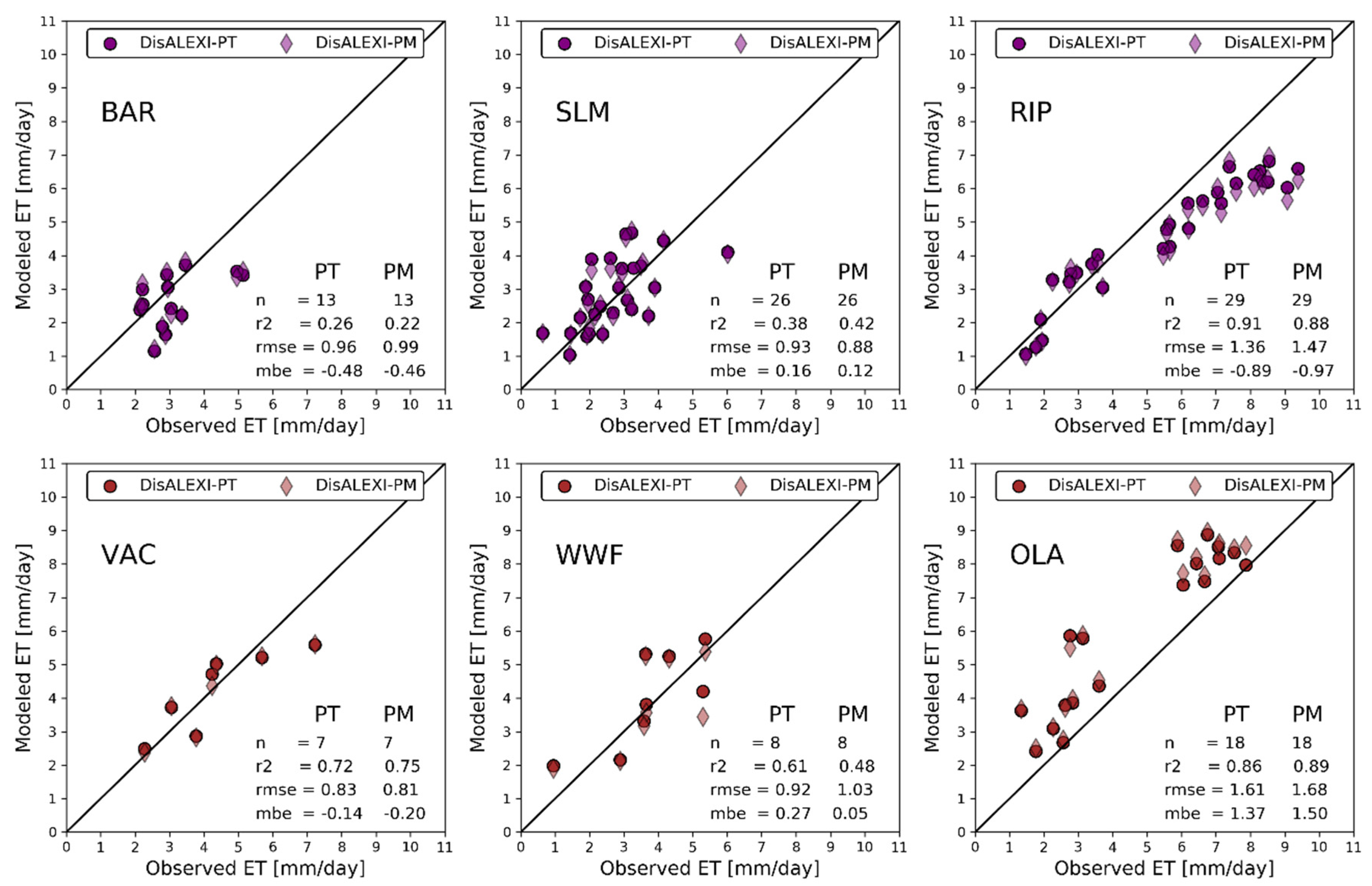
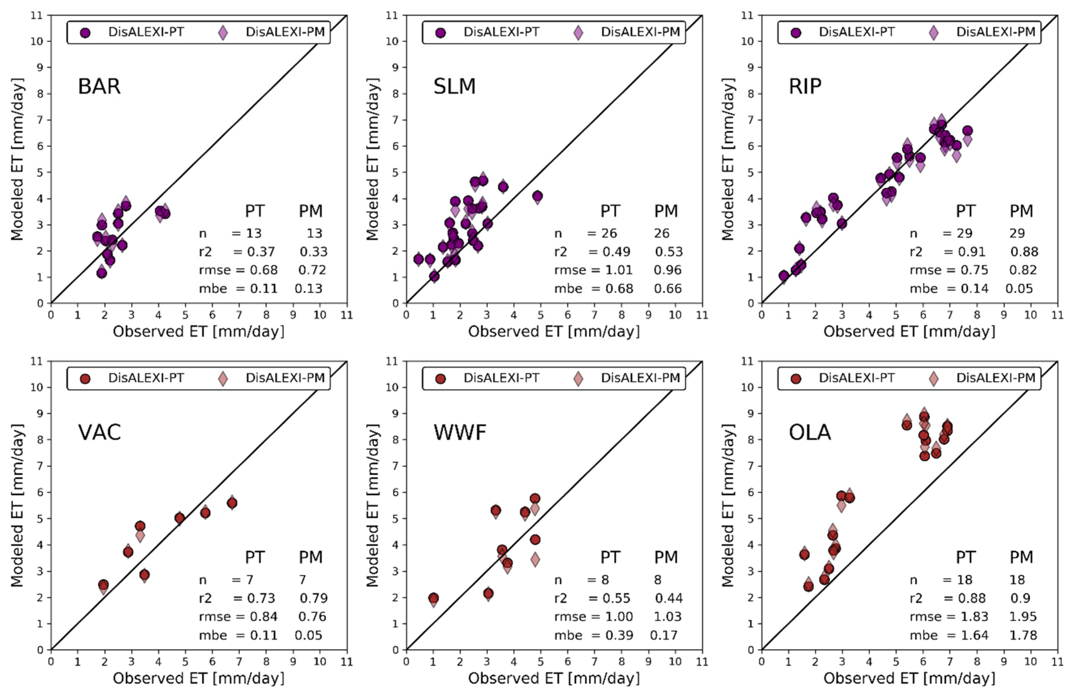
3.1. Evaluation of ALEXI/DisALEXI ET

The ALEXI/DisALEXI modeling scheme has been previously evaluated in California vineyards as part of the GRAPEX project, with resulting daily ET fluxes comparing well with observations (RMSE <= 1.0 mm day⁻¹; [15,16,17,19,58,59,60]). In the current study, we focus on three GRAPEX vineyard sites: BAR, SLM, and RIP. These individual sites were chosen because of their differing cultivars and locations that span the state, offering maximum diversity when making comparisons [6]. The almond orchards used for validation in the current study are VAC, WWF, and OLA and are part of the T-REX project as described in Section 2.1. Although many years of observed data exist at the proposed GRAPEX sites, we focus on 2021 as it overlaps with the availability of observations at the T-REX locations, providing uniformity in what otherwise might be differences in meteorological conditions year to year.

Figure 2 shows the resulting ALEXI/DisALEXI ET values for the Priestley-Taylor-based approach (DisALEXI-PT) and the Penman-Monteith-based approach (DisALEXI-PM) compared against observations for all sites on clear Landsat 8 overpass dates. Vineyard sites are on the top (purple) and almond sites are on the bottom (brown). Observations are taken as the average of multiple energy balance closure techniques as described in [7] and Section 2.2. Unclosed ET observations versus DisALEXI-PT and DisALEXI-PM ET are also shown (Figure 3). The results show good agreement between modeled and closed observed estimates, with an average Root Mean Square Error (rmse) of 1.10 mm day⁻¹ for DisALEXI-PT and 1.14 mm day⁻¹ for DisALEXI-PM on Landsat overpass dates. Although DisALEXI-PT performs slightly better at all sites, small differences in total ET are found between the approaches, regardless of crop or location. The largest errors are reported at sites OLA and RIP, the two southernmost sites. At RIP, errors are due to deviations between the modeled and observed estimates at high values of ET (Figure 2), while a consistent positive bias error is present at OLA.

Modeled negative bias in TSEB for irrigated crops on highly advective days has been noted in previous studies [17,43]. To the northwest of RIP is a large expanse of fallowed land that causes the horizontal advection of hot/dry air across the vineyard, increasing the evaporative demand and causing latent heat fluxes to exceed available energy. These instances lead to large closed estimates of ET (in relation to unclosed) and discrepancies with modeled values as presented in Figure 2. However, when comparing DisALEXI-PT/DisALEXI-PM ET estimates with unclosed values (Figure 3), biases decrease substantially at RIP (from −0.92 to 0.10 mm day⁻¹ on average for DisALEXI-PM and DisALEXI-PT). A similar circumstance is present at VAC, where a large expanse of barren/non-vegetative land (airport) neighbors the orchard, potentially causing the horizontal advection of hot/dry air across the orchard. MBE values are improved at VAC when validating to unclosed ET; however, more datapoints, particularly during high ET days, are required to determine the extent of advective conditions at the site and how closure influences validation efforts. Evaluation between closed and unclosed observations to modeled ET at OLA shows little difference between the two, indicating advective conditions may not be as prevalent at the site, and the modeled positive bias (for both DisALEXI-PT and DisALEXI-PM) is likely due to other factors.

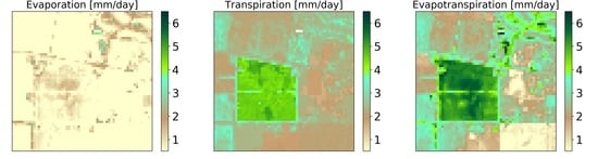
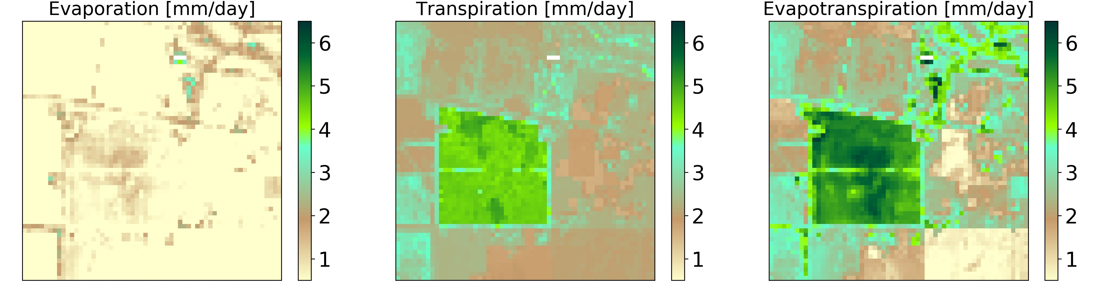
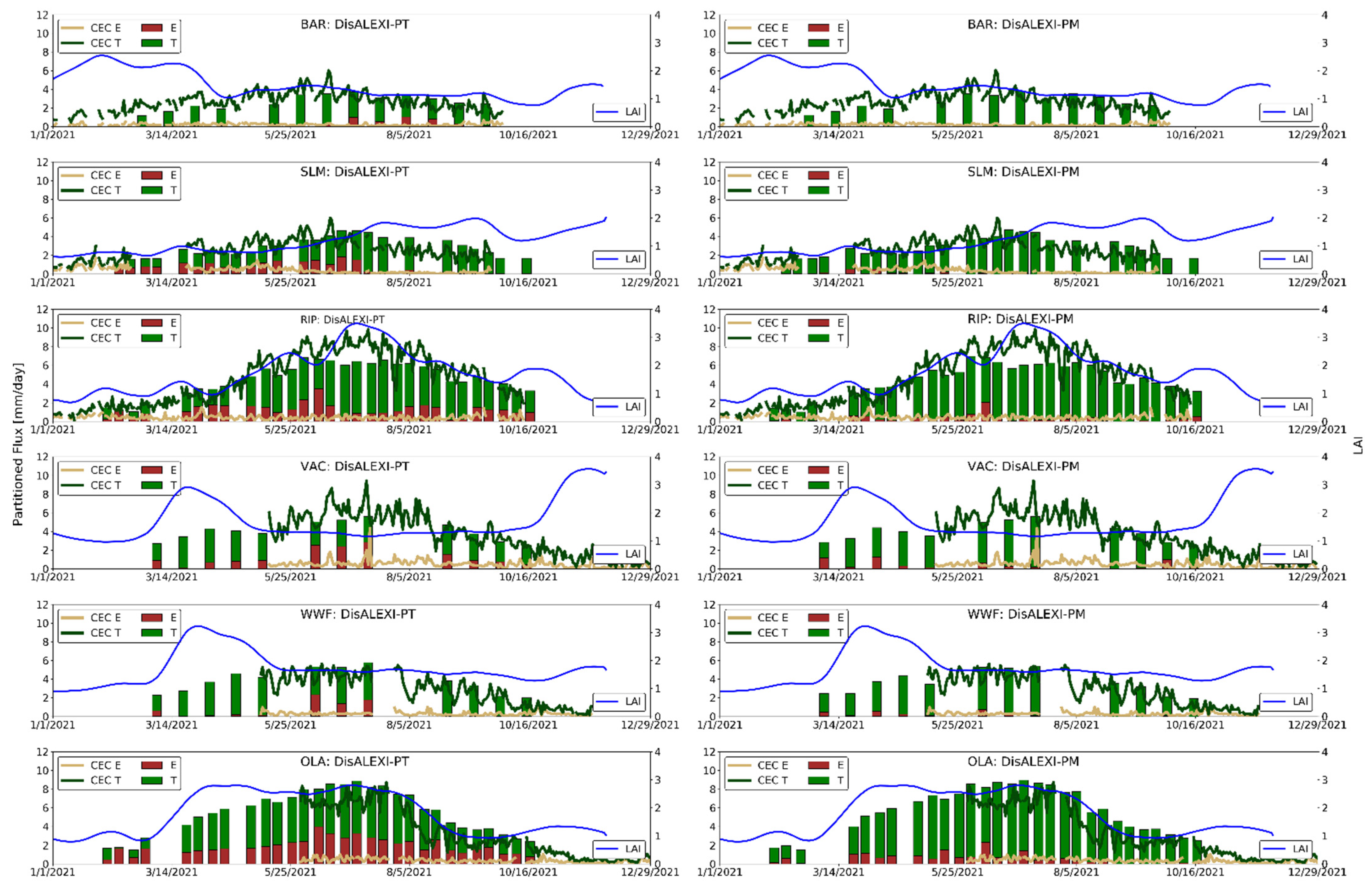
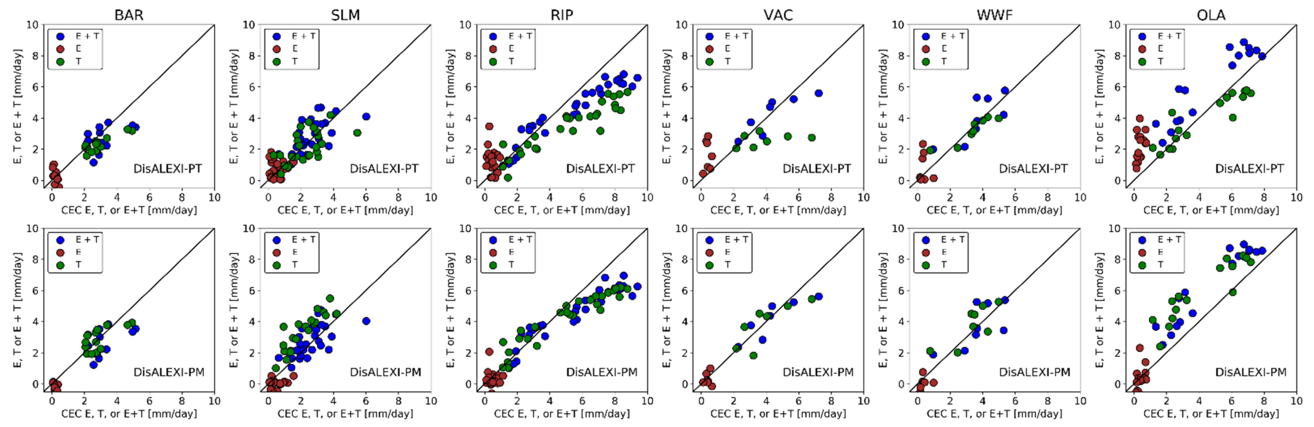
3.2. Evaporation and Transpiration Partitioning

Although daily ET compares well with observations, individual contributions of evaporation (E) and transpiration (T) will provide a better understanding of actual crop water use, particularly in systems with distinct rows and inter-rows. Figure 4 shows a timeseries of these partitioned estimates of E and T for DisALEXI-PT (left) and DisALEXI-PM (right), each denoted as a stacked bar plot, with brown indicating E and green indicating T. Additionally, included are derived E and T estimates (brown and green line, respectively) using the CEC approach as defined in [26] and modeled daily LAI (blue line) from [75].

Timeseries analysis indicates DisALEXI-PT produces elevated estimates of E when compared to CEC E values. This is most notable during the middle of the season, when one would expect E values to be minimal. CEC E values, regardless of the time of year, are close to zero and rarely exceed more than 1 mm day⁻¹. The largest difference between DisALEXI-PT E and CEC E is found at OLA, where DisALEXI-PT E contributes to 34% of the total ET on average over the year. From the timeseries, we find that this percentage increases during June and July, when one would expect E/ET values to decrease or be closer to zero, which is suggested by CEC. It is important to note that OLA is the southernmost site and is exceptionally dry during the summer months (i.e., bare inter-rows with no cover crop). Such a physical setting would suggest little to no E during these months, aligning with CEC-derived E, instead of the elevated values suggested by DisALEXI-PT. Conversely, DisALEXI-PM produces estimates of E that align more closely with CEC-derived E values, with E rarely exceeding 1 mm day⁻¹ regardless of site or time of year. Although muted in comparison, DisALEXI-PM aligns with DisALEXI-PT in that modeled E is highest for site OLA. This trend is only present prior to June, with E values becoming negligible in terms of total ET during the latter half of the year.

In comparison with the E performance, the DisALEXI-PT and DisALEXI-PM-derived T values correlate much better with the CEC-derived T values (Figure 4), except at site RIP during the peak growing season, aligning with the results presented in Figure 2. The DisALEXI-PT and DisALEXI-PM T estimates generally follow annual LAI trends, with values starting low and slowly increasing to peak values during the middle of the year before gradually declining. The decline in T is most abrupt at almond sites, particularly for CEC T, which shows a rapid decrease in T beginning in August. This is a result of irrigation management during a phenological period called hull split. When the almond splits and exposes the soft shell inside (hull split), it leaves the almond more vulnerable to diseases such as hull rot [76]. To limit damage, growers reduce irrigation to promote the drying out of the nuts and to shorten the window of time where the orchard is vulnerable to damage, causing estimates of T (and ET) to decrease. Although the DisALEXI-PT and DisALEXI-PM T values decrease in response to hull split, they fail to match the magnitude of the decline, remaining ~2 mm day⁻¹ higher than the estimates provided by CEC (for site OLA where Landsat imagery is available).

Scatter plots between the modeled and observed partitioned fluxes show similar patterns (Figure 5). Specifically, we find clear discrepancies between DisALEXI-PT and DisALEXI-PM E partitioning, with the latter more closely aligning with CEC E (Figure 5, bottom row) and the former often overestimating (Figure 5, top row) with an overall MBE = 0.88 mm day⁻¹ (

Table 2. Statistical metrics correlation coefficient (R²), root mean square error (RMSE), and mean bias error (MBE) for DisALEXI-PT (PT) and DisALEXI-PM (PM) partitioned evaporation (E), transpiration (T), and combined E and T compared to CEC-derived E and T and combined E and T for all sites.

	E		T		E + T
	PT	PM	PT	PM	PT	PM
R2	0.03	0.04	0.77	0.70	0.75	0.72
RMSE (mm/day)	1.26	0.64	0.82	1.41	1.25	1.30
MBE (mm/day)	0.88	−0.23	−0.07	1.02	0.80	0.79
MAE (mm/day)	0.97	0.45	0.57	1.11	0.96	0.99

) as the CEC E remains consistently small (<1 mm day⁻¹). In contrast, the T estimates from DisALEXI-PT generally align with the CEC T, with an MBE of −0.07 mm day⁻¹ when averaged over all sites, where DisALEXI-PM yields an MBE of 1.02 mm day⁻¹_. The DisALEXI-PM T estimates perform best at sites RIP and VAC, coinciding with worse DisALEXI-PT T performance. Such a result is expected as RIP and VAC are most prone to advective conditions. Focusing on VAC for days with high ET (≥4 mm day⁻¹; Landsat overpass dates of 9 June, 25 June, and 11 July 2021) shows nearly identical total ET estimates for DisALEXI-PT and DisALEXI-PM. However, DisALEXI-PT suggests T/ET ratios close to ~0.5, meaning E is contributing ~50% to total water use during this time period. This amount of E is not likely to occur given the dry barren interrow present during the summer at VAC. Conversely, DisALEXI-PM suggests T/ET ratios closer to 1.0. This same pattern, albeit less drastic, is seen at RIP, where the DisALEXI-PT T values show negative bias with the CEC T for values ≥ 4 mm day⁻¹, while the DisALEXI-PM T shows better alignment for the same values. At site OLA, we find DisALEXI-PM overestimates T (aligning with CEC E) and DisALEXI-PT overestimates E (aligning with CEC T), contributing to both estimating similar total ET estimates (Figure 5).

As described in Section 2.3.2, a major difference between DisALEXI-PT and DisALEXI-PM is how the T_c at the satellite overpass time is calculated when solving the temperature gradient–resistance system of the equations. Therefore, differences in E or T from DisALEXI-PT or DisALEXI-PM propagate from estimates of T_c. Additionally, past research has shown that the effect advection, and by proxy, VPD, can have on estimates of T [33,43]. Figure 6 compares the DisALEXI-PT and DisALEXI-PM T_c estimates with T_a (initial estimate used as model input) and VPD (calculated using T_a and CFSR vapor pressure). The results suggest a common trend, with T_c (y-axis) and VPD (color scale) increasing with an increase in T_a for all sites and both approaches (Figure 6A,B). In both models, T_c follows a linear correlation with T_a, with values between 0 to ~2 °C warmer than T_a throughout most of the year and regardless of site. However, there are specific instances when T_c is reported as less than T_a, a characteristic of dry air advection. These instances are only identified in DisALEXI-PM-derived T_c values (Figure 6B); the DisALEXI-PT T_c estimates always remain ≥T_a (Figure 6A). Instances of T_c ≤ T_a tend to align with higher VPD (red tones), with more occurrences at higher T_a values. However, there are instances when T_c ≤ T_a even at cooler temperatures (T_a ≤ 25 °C). Closer inspection indicates a division between T_c and VPD for instances of T_c ≤ T_a (Figure 6C, red) and T_c ≥ T_a (DisALEXI-PM = blue, DisALEXI-PT = green; Figure 6C). This is because DisALEXI-PM accounts for the effects of elevated VPD via its explicit inclusion within the framework (see Equation (10)), whereas DisALEXI-PT assumes that the influence of VPD is mostly accounted for in the α parameter. Most instances of T_c ≤ T_a link to the large differences in the DisALEXI-PT and DisALEXI-PM T estimates discussed above and shown in Figure 6. Specifically, the improvement in T estimation by DisALEXI-PM compared to DisALEXI-PT for RIP and VAC for values ≥ 4 mm day⁻¹ align with instances of T_c < T_a (not shown), suggesting the improvement in these cases is related to VPD inclusion.

Figure 7 shows a comparison between the DisALEXI-PT and DisALEXI-PM estimates of T_c (top left) and T_s (bottom left), as well as the major individual energy balance flux components, demonstrating how differences in T_c influence and propagate to differences in E and T between approaches. Note that energy balance component values are at Landsat overpass times and are given in units of W m⁻². Accordingly, E and T are presented as λE_s and λE_c, respectively. Additionally included is the average difference between component values (PM minus PT).

DisALEXI-PM produces T_c values that are 5.3 °C cooler, on average, than DisALEXI-PT estimates. Cooler T_c values result in T_s values that are 4.6 °C warmer, on average, than DisALEXI-PT estimates. Cooler T_c and warmer T_s DisALEXI-PM predictions propagate to an increase in R_nc (+15 W m⁻²) and a decrease in R_ns (−16 W m⁻²) when compared to estimates proposed by DisALEXI-PT (Figure 7). The canopy (H_c) and soil (H_s) sensible heat flux contributions show a change between −60 W m⁻² for H_c and +62 W m⁻² for H_s, with the values of H_c highlighting the ability of DisALEXI-PM to capture negative H values. In combination, these differences lead to DisALEXI-PM canopy transpiration rates (λE_c) roughly 30% larger than those from DisALEXI-PT (+75 W m⁻²). The differences in soil evaporation (λE_s) are opposite in sign, with DisALEXI-PM yielding λE_s estimates that are ~80% smaller (−76 W m⁻²) than the DisALEXI-PT estimates. Conversion to daily mass units for reference with previously discussed E and T estimates results in DisALEXI-PM producing 2.64 mm day⁻¹ more transpiration and 2.68 mm day⁻¹ less evaporation than DisALEXI-PT when averaged for all sites.

Another notable difference between DisALEXI-PT and DisALEXI-PM is the use of r_c within the DisALEXI-PM framework. To be consistent with the original PM version of TSEB implemented by [38], r_c is held constant at 50 s m⁻¹ (see Section 2.3.2). However, this value represents a reference short crop (i.e., well-watered and full canopy), which may cause issues in taller and/or more heterogeneous canopies where the sensitivity of r_c to VPD will be more significant. To evaluate the model’s sensitivity to r_c, we ran DisALEXI-PM using incrementally increasing r_c values (10 to 95 s m⁻¹) and calculated the error in T, E, and ET (Figure 8). Figure 7 shows the mean bias error (MBE; mm day⁻¹) between the DisALEXI-PM-derived T, E, or ET and the CEC-derived T or E (green and brown bar, respectively) for each model run (defined by the value of r_c; x-axis). Additionally included is the combined ET modeled bias (Figure 7; black line with yellow highlight).

The results suggest that an increase in r_c causes modeled E values to increase (negative to positive bias) and T values to decrease (bias becoming less positive). This is expected as an increase in r_c while holding VPD constant will result in decreasing T. Accordingly, the largest improvements in MBE achieved by increasing r_c are found at RIP and VAC, where advection is more common, and at OLA, where a more substantial overestimation of T was originally derived (i.e., a decrease in modeled T inherently improves error predictions). Figure 8 suggests that DisALEXI-PM E and T estimates would benefit from site-specific r_c values better representing surface conditions as biases in T decrease to minimums at different r_c values. Note that minimal biases in T do not explicitly align with minimal biases in E. Although magnitudes are different, decreases in T bias align with an increase in E bias. When combined as ET, we find little difference in the modeled bias (Figure 8; black line with yellow highlight), suggesting changes in r_c have an effect on partitioned fluxes but offer little improvement in the modeled total ET. Declining T biases corroborate results presented in [43], where a partitioning algorithm that included an r_c formula that relates maximum stomata conductance to VPD produced the most reasonably partitioned estimates of E and T.

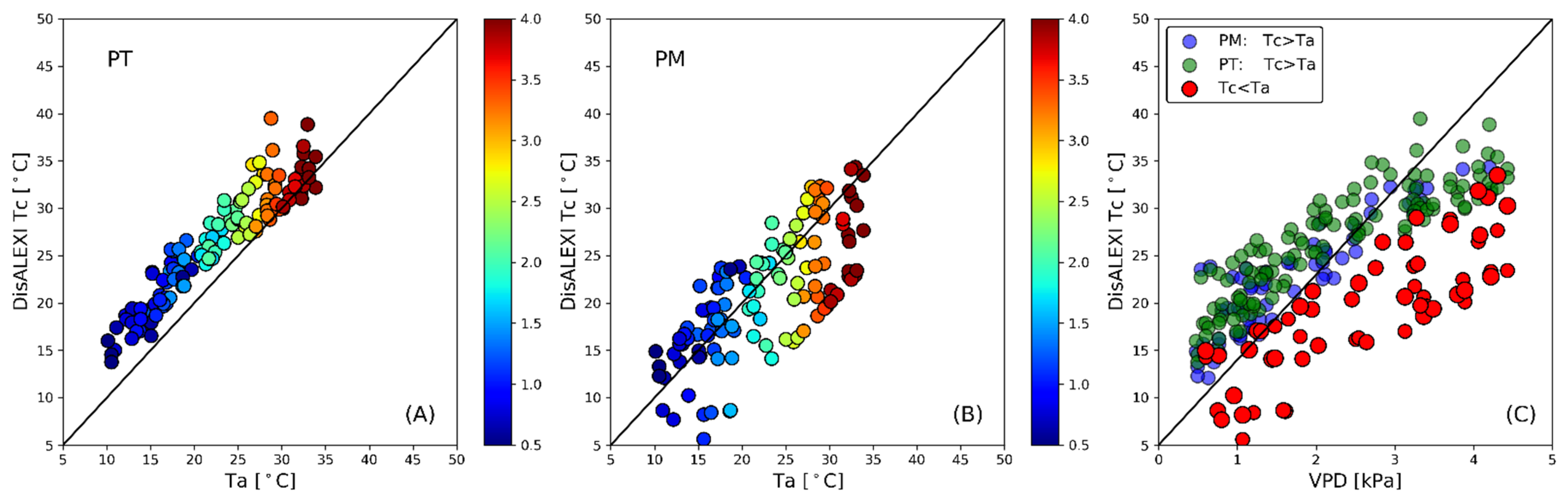
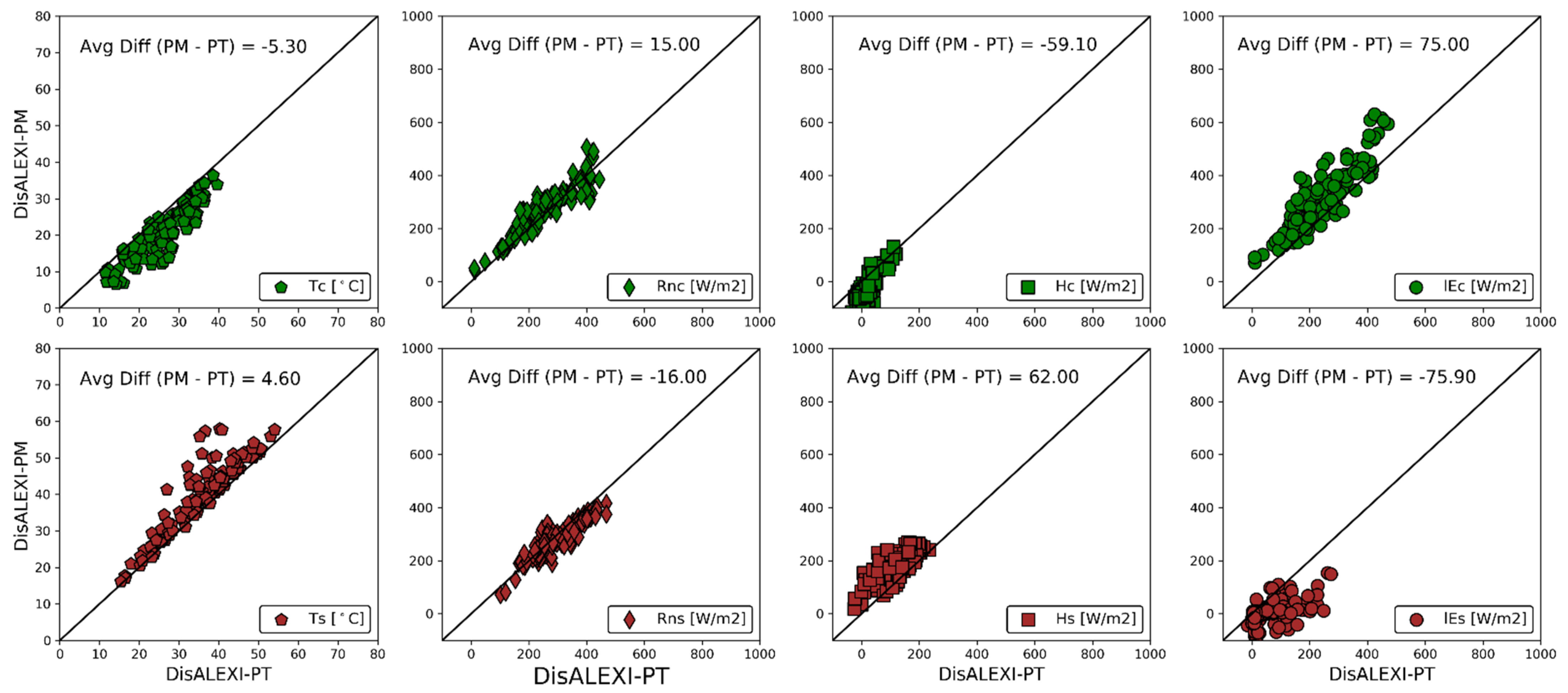
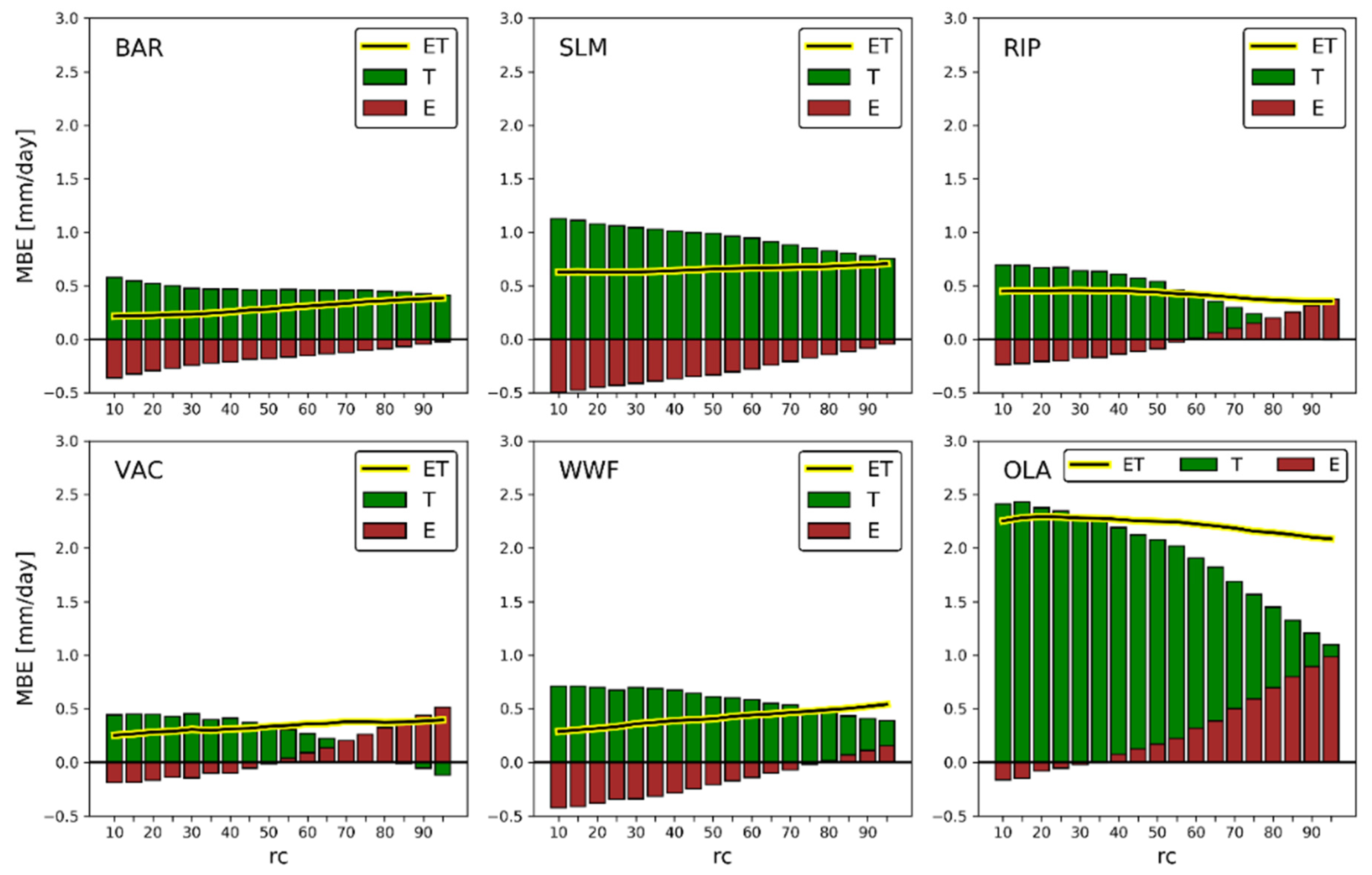
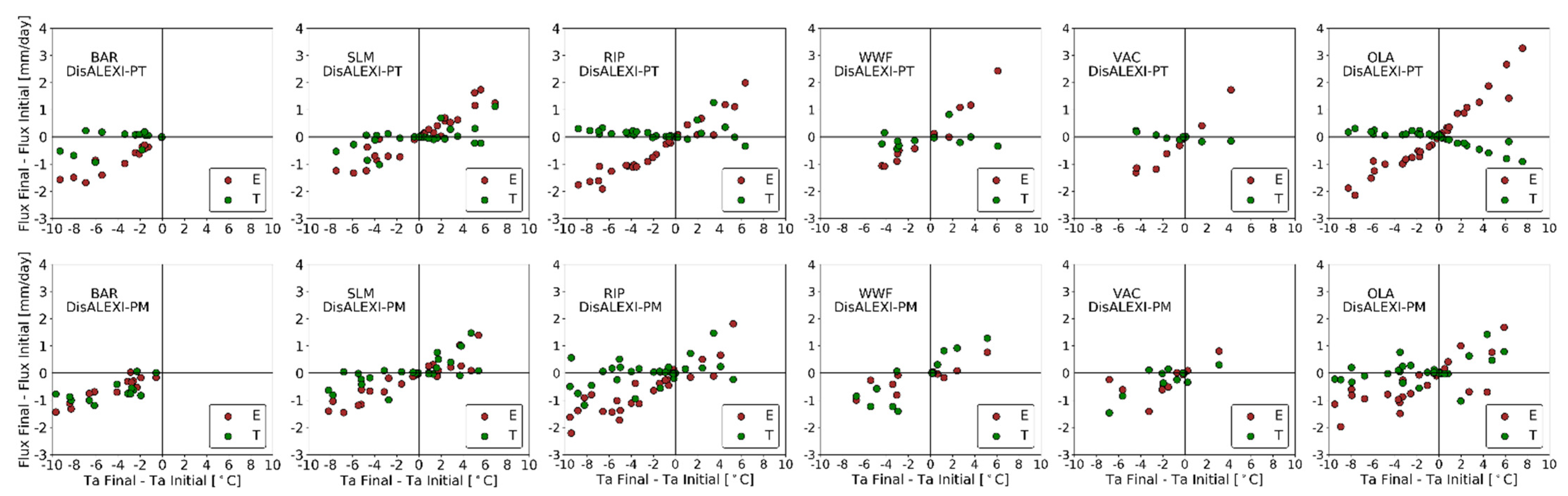
3.3. ALEXI/DisALEXI Iterations of TSEB

To ensure consistency between the ALEXI and DisALEXI ET estimates, the T_a is iteratively adjusted at the ALEXI pixel scale until the DisALEXI daily ET, spatially averaged over the ALEXI pixel, converges to the ALEXI value. This iterative process requires running TSEB on each iteration. Under the TSEB system of equations (DisALEXI-PT or DisALEXI-PM), adjustments to the T_a will change the T_c and T_s and subsequently, T and E. Such a process may result in unrealistic estimates of T and E partitioning even though components may sum to reasonable estimates of ET. One such case may be under conditions of strong advection over irrigated crops, where deviations between DisALEXI and ALEXI ET may be impacted more by the horizontal advection of energy rather than air temperature boundary conditions at the blending height. Given the iterative process associated with DisALEXI, we evaluate the behavior of E and T by comparing the difference between the final and initial estimates of E and T (Figure 9, y-axis) with the difference between the final and initial T_air (Figure 9, x-axis) for DisALEXI-PT (Figure 9, top row) and DisALEXI-PM (Figure 9, bottom row).

An evaluation of Figure 9 shows distinct patterns in the DisALEXI-PT E and T response to T_a, quantified with respect to values obtained from the initial T_a boundary conditions obtained from CFSR (Figure 9, top row). The pattern can best be observed at OLA, where differences in T_a more directly influence the E values compared to T. In general, as T_a increases, H will decrease as the surface-to-air temperature gradient reduces, subsequently leading to an increase in ET (E+T) to maintain energy balance. The inverse response is expected as T_a decreases. Although the response from the individual E and T components is also dependent on specific site conditions (e.g., vegetation cover, stress, etc.), convergence on the ALEXI ET appears primarily driven by shifts in E for the DisALEXI-PT approach. Conversely, the DisALEXI-PM model results show more uniformity in E and T component responses to shifts in T_a (Figure 9, bottom row), suggesting more proportionate adjustments to E and T in relation to ET.

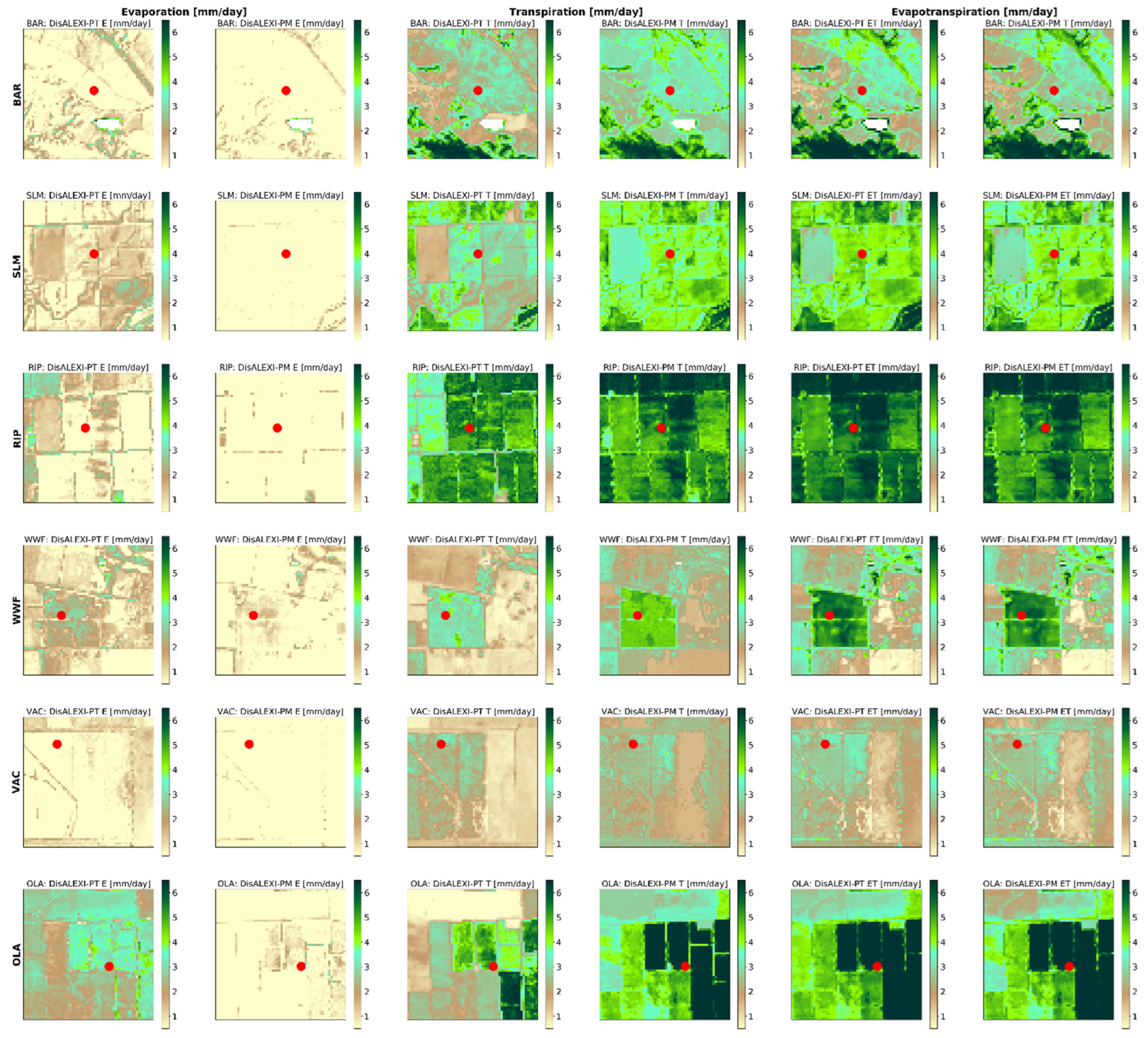
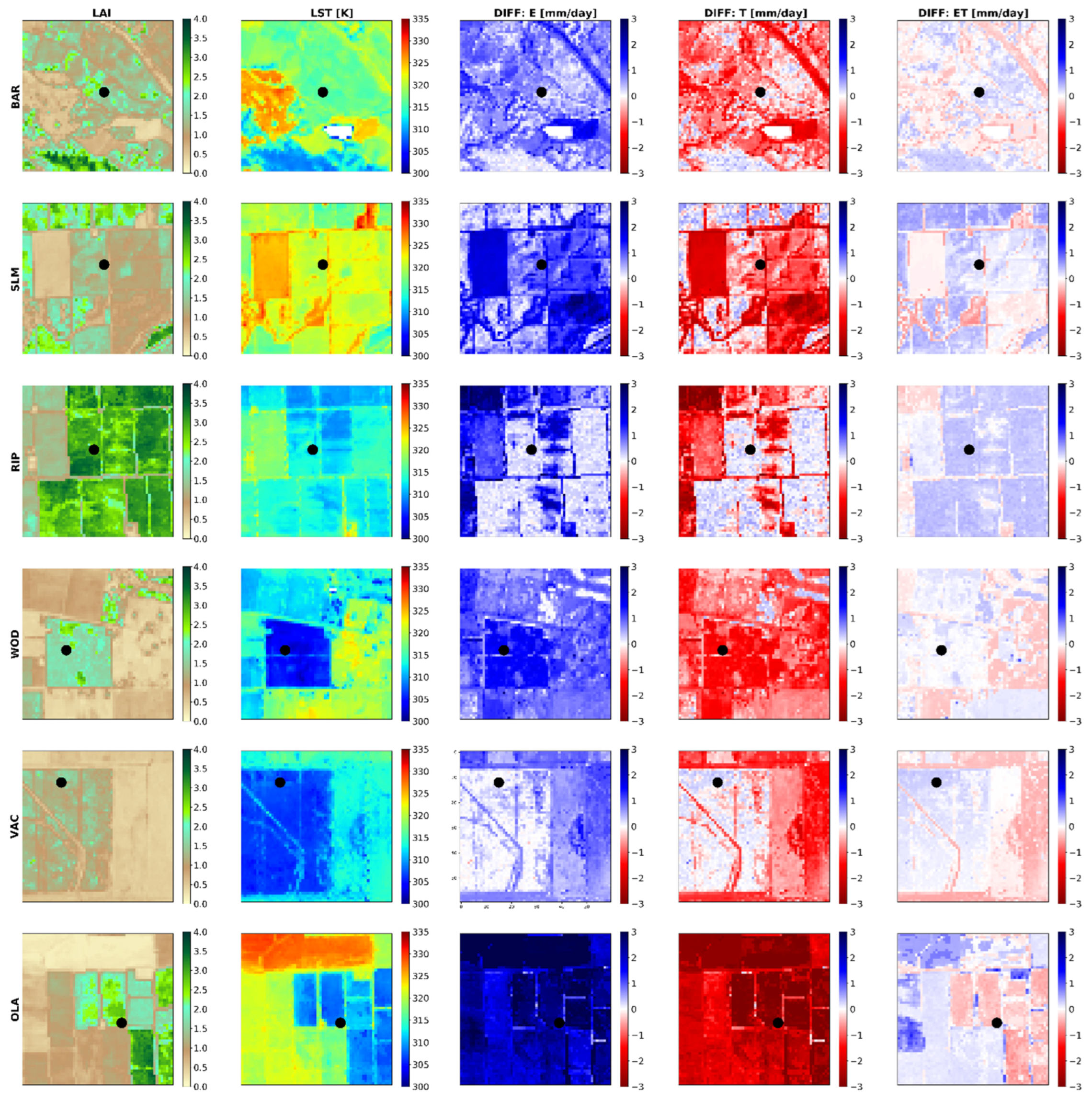
3.4. Spatial Analysis

A key advantage of the ALEXI/DisALEXI modeling framework is the spatial component—producing daily ET estimates over expansive areas that may encompass multiple vineyards, orchards, or other commodities. Figure 10 provides a contextual look at the mapping of ET, as well as E and T, by both models over multiple sites. These maps were created using Landsat-8 data collected during the month of June in 2021 (BAR = 06/16, SLM = 06/18, RIP = 06/18, OLM = 06/18, VAC = 06/09, WOD = 06/09). The red dots indicate the tower’s location within the vineyard or orchard. These maps reflect tendencies discussed above, with DisALEXI-PM generally generating lower/higher estimates of E/T than DisALEXI-PT, despite the similarity in the representation of total ET.

The differences between the DisALEXI-PT- and DisALEXI-PM-derived E, T, and ET for all sites on the same dates are shown in Figure 11. Additionally included are LAI and LST images on the same dates, acquired at the Landsat overpass time. The differences in E are lowest over BAR and VAC and greatest at OLA (differences ≥ 2 mm day⁻¹ over most of the area). The areas of strongest difference in T and E between the models tend to occur where the LAI is low and the LST is high. The most extreme case is found in the field directly to the west of SLM, where the LAI values are the lowest (~0.5) and the LST values are the highest (~52 °C). This combination results in low ET for both DisALEXI-PT and DisALEXI-PM (Figure 10, right two columns), with little difference between the two (Figure 11). However, a comparison between E and T suggests total ET from DisALEXI-PT over this field is primarily driven by evaporation, whereas for DisALEXI-PM, it is primarily driven by transpiration. Although no ground-truth instrumentation exists for this field, visual inspection indicates a newly planted vineyard, characteristic of having little vine biomass and drip irrigation installed. If irrigation is substantial and creates a wetted soil, E is likely to contribute a larger fraction to ET, aligning with the DisALEXI-PT results. Although differences in E and T are nearly equal and opposite for most areas surrounding the sites, spatial patterns indicate that DisALEXI-PT produces larger ET estimates over areas of higher LAI and lower LST (except for OLA) on these dates when compared to DisALEXI-PM (Figure 10). In terms of total ET between DisALEXI-PT and DisALEXI-PM, we find little difference between the approaches, with values remaining ≤ 0.75 mm day⁻¹ in either direction, aligning with the results presented in the prior sections.

4. Discussion

The evaluation of DisALEXI-PT and DisALEXI-PM indicates little difference in the magnitude and accuracy of their daily total ET estimates when compared to observations at vineyard and orchard sites. However, the evaluation of contributions from individual fluxes E and T for DisALEXI-PT and DisALEXI-PM show considerable differences, both in comparison to CEC-derived fluxes and to one another. As the name of each implies, DisALEXI-PT and DisALEXI-PM differ in the initial and subsequently iteratively adjusted derivation of T_c, with DisALEXI-PT using a modified Priestley-Taylor approach and DisALEXI-PM using the Penman-Monteith. Such a difference allows VPD, and potential advective conditions, to be explicitly accounted for in the DisALEXI-PM approach (omitted in DisALEXI-PT). Aligning with past studies [38,40,43], DisALEXI-PM performs best under advective conditions (sites RIP and VAC) when analyzing partitioned E and T estimates. However, regardless of differences in E and T, summation equates to analogous DisALEXI-PT and DisALEXI-PM total ET estimates, suggesting advective conditions only affect partitioned estimates and not total ET within the proposed modeling frameworks. Improvements in DisALEXI-PM-derived E and T can be attained by utilizing more site-specific r_c values rather than holding the r_c constant at 50 s m⁻¹. These results align with [43], where TSEB based on the Penman-Monteith formulation overestimated T, but TSEB based on utilizing a site-specific r_c value improved T estimates. Work is underway to address this limitation within the DisALEXI-PM approach by implementing the results of [43] within the DisALEXI framework, including the transition of site-specific, empirically driven relationships into more physically based relationships that can be applied at scale, similar to [77].

Under drought conditions and the threat of continued water restrictions for agricultural irrigation in the state of California, many parcels of land are being fallowed, creating more instances of irrigated cropland adjacent to dry barren parcels of land. Such a situation is likely to lead to increased horizontal advection of hot/dry air across irrigated fields, increasing the evaporative demand and causing latent heat fluxes to exceed available energy over irrigated fields. Therefore, careful consideration should be taken when validating satellite-based ET models over California. An example of such an instance was shown at site RIP, where advective conditions caused large differences between the closed and unclosed observed ET. A comparison of the DisALEXI-PT- and DisALEXI-PM-derived ET to the observed ET at RIP showed a strong negative bias to the energy-balanced closed ET estimates for high ET values (ET ≥ 4 mm day⁻⁴), whereas the biases improved greatly when compared to the unclosed estimates for the same time period.

DisALEXI-PT and DisALEXI-PM similarly adjust T_a until the aggregated ET converges with the ALEXI ET. However, given differences in the derivation of T_c, these T_a adjustments will affect T_c and T_s, and by association, T and E differently. The results suggest that the DisALEXI-PM ET values converge on the ALEXI ET with more proportionate adjustments to E and T, whereas the DisALEXI-PT convergence is primarily met with adjustments to E, the exception being when soil evaporation is ≤ 0 and the Priestley-Taylor term (α) is allowed to change from its initially assigned value (Equation (4)). Therefore, conditions leading to large differences between the ALEXI ET and the initial aggregated ET can have large ramifications. Specifically, if the ALEXI ET is considerably larger than the aggregated ET, DisALEXI-PT will adjust by increasing E. In vineyard and almond systems, where distinct differences are present between the drip-irrigated canopy and non-irrigated soil, this may lead to inappropriately high E values. Conversely, when the ALEXI ET is much lower than the aggregated ET, DisALEXI-PT will adjust by decreasing E, producing reasonable partitioned estimates of E during the growing season. However, should these conditions be met in the spring, when the soil moisture content is larger [78,79,80], decreases in E may be excessive. The incorporation of DisALEXI-PM may provide a solution by adjusting E and T more proportionately. Large differences between ALEXI ET and disaggregated ET were not found during the current study. Future work will look to identify ALEXI pixels displaying large biases to disaggregated ET based on surface spatial heterogeneity and/or time of year and test differences between the DisALEXI-PT and DisALEXI-PM approaches.

Spatial analysis mirrors patterns found at the field scale, with DisALEXI-PT showing elevated E in comparison to DisALEXI-PM, which indicates E values closer to zero over each site and for most of the surrounding area (Figure 10). Estimates of T are opposite in relation, with DisALEXI-PM producing larger T estimates over each site and over surrounding fields. DisALEXI-PT shows more range in T, particularly for low values. The summation of E and T for both approaches produces analogous ET estimates, with differences of ≤0.75 mm day⁻¹ in either direction over the regions shown. Such maps demonstrate the differences in the partitioned E and T between approaches despite the similarities in total ET values. In water-limited agronomic systems where distinct differences are present between the soil (likely dry during the growing season) and canopy (direct application of irrigation leading to full canopies), differentiation between E and T is required for improved irrigation management.

5. Conclusions

The mapping of ET and its individual components of surface evaporation (E) and canopy-based transpiration (T) at spatial scales suitable for irrigation management has the potential to lead efforts in the conservation of agricultural water resources and improve irrigation and water use efficiencies in water-limited systems. This study evaluated the partitioning of E and T within the context of the ALEXI/DisALEXI modeling framework using a modified Priestley-Taylor approach (DisALEXI-PT) and a Penman-Monteith approach (DisALEXI-PM). Analysis was performed over three wine grape vineyard sites and three almond orchard sites all located in California for the year 2021. The sites are primary targets of micrometeorological and biophysical field measurements as part of the USDA-ARS Grape Remote sensing Atmospheric Profile and Evapotranspiration eXperiment (GRAPEX) and Tree Remote sensing of Evapotranspiration eXperiment (TREX) projects.

The results indicate that the DisALEXI-PM approach estimates canopy temperatures roughly 5 °C cooler and soil temperatures roughly 5 °C warmer when compared to DisALEXI-PT (average for all sites). These temperature differences cause subsequent differences in evaporation (E) and transpiration (T) values, with DisALEXI-PM producing E values 2.69 mm day⁻¹ lower and T values 2.64 mm day⁻¹ higher than those estimated by DisALEXI-PT. The differences are in part due to DisALEXI-PM accounting for the effects of VPD, allowing T_c to decrease and subsequently T to increase under more advective conditions. DisALEXI-PT does not have a mechanism to increase T in such a way. The evaluation of the iterative process required for ALEXI/DisALEXI indicates that the DisALEXI-PM ET values converge on the ALEXI ET with more proportionate adjustment to E and T, whereas the DisALEXI-PT convergence is primarily driven by adjustments to E. Such a difference may present misguided partitioned fluxes, should the ALEXI ET and the disaggregated DisALEXI ET be considerably different. Improvement in the DisALEXI-PM-derived E and T estimates can be attained by incorporating r_c values defined by local surface conditions rather than holding constant at 50 s m⁻¹. Spatial analysis aligns with tower-based evaluations, suggesting that the resulting differences in E and T between the approaches are also found over areas surrounding each study site.

In water-limited agricultural systems where distinct differences between the soil and canopy are prevalent, it is important to accurately partition ET into individual contributions of E and T as the irrigation strategy is likely to focus on reducing water loss from E rather than T. The analysis presented here has the potential to drive improvements in the ALEXI/DisALEXI modeling framework to provide more specific soil- and canopy-consumptive water use information in unique canopy structures characteristic of irrigated woody perennial crops, allowing for improved irrigation and water use efficiencies in these water-limited systems.

References

1. Flörke, M.; Schneider, C.; McDonald, R.I. Water competition between cities and agriculture driven by climate change and urban growth. Nat. Sustain. 2018, 1, 51–58. [Google Scholar] [CrossRef]
2. Faunt, C.C.; Sneed, M.; Traum, J.; Brandt, J.T. Water availability and land subsidence in the Central Valley, California, USA. Hydrogeol. J. 2016, 24, 675–684. [Google Scholar] [CrossRef] [Green Version]
3. Scanlon, B.R.; Reedy, R.C.; Faunt, C.C.; Pool, D. Enhancing drought resilience with conjunctive use and managed aquifer recharge in California and Arizona. Environ. Res. Lett. 2016, 11, 035013. [Google Scholar] [CrossRef] [Green Version]
4. Kustas, W.P.; Anderson, M.C.; Alfieri, J.G.; Knipper, K.; Torres-Rua, A.; Parry, C.K.; Nieto, H.; Agam, N.; White, W.A.; Gao, F. The grape remote sensing atmospheric profile and evapotranspiration experiment. Bull. Am. Meteorol. Soc. 2018, 99, 1791–1812. [Google Scholar] [CrossRef] [Green Version]
5. Agam, N.; Kustas, W.P.; Alfieri, J.G.; Gao, F.; McKee, L.M.; Prueger, J.H.; Hipps, L.E. Micro-scale spatial variability in soil heat flux (SHF) in a wine-grape vineyard. Irrig. Sci. 2019, 37, 253–268. [Google Scholar] [CrossRef]
6. Bambach, N.; Kustas, W.; Alfieri, J.; Gao, F.; Prueger, J.; Hipps, L.; McKee, L.; Castro, S.J.; Alsina, M.M.; McElrone, A.J. Inter-annual variability of land surface fluxes across vineyards: The role climate, phenology, and irrigation management. Irrig. Sci. 2022, 40, 463–480. [Google Scholar] [CrossRef]
7. Bambach, N.; Kustas, W.P.; Alfieri, J.G.; Hipps, L.E.; McKee, L.; Castro, S.J.; Volk, J.; Alsina, M.M.; McElrone, A.J. Evapotranspiration uncertainty at micrometeorological scales: The impact of the eddy covariance energy imbalance and correction methods. Irrig. Sci. 2022, 40, 445–461. [Google Scholar] [CrossRef]
8. Alfieri, J.; Kustas, W.P.; Prueger, J.H.; McKee, L.G.; Hipps, L.E.; Bambach, N. The vertical turbulent structure within the surface boundary layer above a vineyard in California’s Central Valley during GRAPEX. Irrig. Sci. 2022, 40, 481–496. [Google Scholar] [CrossRef]
9. Xia, T.; Kustas, W.P.; Anderson, M.C.; Alfieri, J.G.; Gao, F.; McKee, L.; Prueger, J.H.; Geli, H.M.E.; Neale, C.M.U.; Sanchez, L.; et al. Mapping evapotranspiration with high-resolution aircraft imagery over vineyards using one- and two-source modeling schemes. Hydrol. Earth Syst. Sci. 2016, 20, 1523–1545. [Google Scholar] [CrossRef] [Green Version]
10. Nieto, H.; Kustas, W.P.; Torres-Rúa, A.; Alfieri, J.G.; Gao, F.; Anderson, M.C.; White, W.A.; Song, L.; Alsina, M.M.; Prueger, J.H.; et al. Evaluation of TSEB turbulent fluxes using different methods for the retrieval of soil and canopy fluxes using different methods for the retrieval of soil and canopy component temperatures from UAV thermal and multispectral imagery. Irrig. Sci. 2019, 37, 389–406. [Google Scholar] [CrossRef]
11. Aboutalebi, M.; Torres-Rúa, A.F.; Kustas, W.P.; Nieto, H.; Coopmans, C.; McKee, M. Assessment of different methods for shadow detection in high-resolution optical imagery and evaluation of shadow impact on calculation of NDVI, and evapotranspiration. Irrig. Sci. 2019, 37, 407–429. [Google Scholar] [CrossRef]
12. Torres-Rúa, A.; Nieto, H.; Parry, C.; Elarab, M.; Collatz, W.; Coopmans, C.; McKee, L.; McKee, M.; Kustas, W.P. Inter-comparison of thermal measurements using ground-based sensors, UAV thermal cameras, and eddy covariance radiometers. Proc. SPIE Int. Soc. Opt. Eng. 2018, 10664, 105–116. [Google Scholar]
13. Torres-Rúa, A.; Ticlavilca, A.M.; Aboutalebi, M.; Nieto, H.; Alsina, M.M.; White, A.; Prueger, J.H.; Alfieri, J.G.; Hipps, L.E.; McKee, L.G.; et al. Estimation of evapotranspiration and energy fluxes using a deep-learning-based high-resolution emissivity model and the Two-Source Energy Balance Model with sUAS Information. Proc. SPIE 2020, 11414, 61–75. [Google Scholar]
14. Nassar, A.; Torres-Rúa, A.; Kustas, W.P.; Nieto, H.; McKee, M.; Hipps, L.; Stevens, D.; Alfieri, J.; Prueger, J.; Alsina, M.M.; et al. Influence of model grid size on the estimation of surface fluxes using the Two Source Energy Balance Model and sUAS imagery in vineyards. Remote Sens. 2020, 12, 342. [Google Scholar] [CrossRef] [Green Version]
15. Semmens, K.A.; Anderson, M.C.; Kustas, W.P.; Gao, F.; Alfieri, J.G.; McKee, L.; Prueger, J.H.; Hain, C.R.; Cammalleri, C.; Yang, Y.; et al. Monitoring daily evapotranspiration over two California vineyards using Landsat 8 in a multi-sensor data fusion approach. Remote Sens. Environ. 2016, 185, 155–170. [Google Scholar] [CrossRef] [Green Version]
16. Knipper, K.R.; Kustas, W.P.; Anderson, M.C.; Alfieri, J.G.; Prueger, J.H.; Hain, C.R.; Gao, F.; Yang, Y.; McKee, L.G.; Nieto, H. Evapotranspiration estimates derived using thermal-based satellite remote sensing and data fusion for irrigation management in California vineyards. Irrig. Sci. 2019, 37, 431–449. [Google Scholar] [CrossRef]
17. Knipper, K.R.; Kustas, W.P.; Anderson, M.C.; Nieto, H.; Alfieri, J.G.; Prueger, J.H.; Hain, C.R.; Gao, F.; McKee, L.G.; Alsina, M.M.; et al. Using high-spatiotemporal thermal satellite ET retrievals to monitor water use over California vineyards of difference climate, vine variety and trellis design. Agric. Water Manag. 2020, 241, 106361. [Google Scholar] [CrossRef]
18. Bhattarai, N.; D’Urso, G.; Kustas, W.P.; Bambach, N.; Anderson, M.; McElrone, A.J.; Knipper, K.R.; Gao, F.; Alsina, M.M.; Aboutalebi, M.; et al. Influence of modeling domain and meteorological forcing data on daily evapotranspiration estimates from a Shuttleworth–Wallace model using Sentinel-2 surface reflectance data. Irrig. Sci. 2022, 40, 497–513. [Google Scholar] [CrossRef]
19. Knipper, K.R.; Kustas, W.P.; Anderson, M.C.; Alsina, M.M.; Hain, C.R.; Alfieri, J.G.; Prueger, J.H.; Gao, F.; McKee, L.G.; Sanchez, L.A. Using high-spatiotemporal thermal satellite ET retrievals for operational water use and stress monitoring in a California vineyard. Remote Sens. 2019, 11, 2124. [Google Scholar] [CrossRef] [Green Version]
20. Doorenbos, J.; Kassam, A.H. Yield response to water. In Irrigation and Drainage Paper No. 33; Unite Nations FAO: Rome, Italy, 1979. [Google Scholar]
21. Fereres, E.; Soriano, M.A. Deficit irrigation for reducing agricultural water use. J. Exp. Bot. 2007, 58, 147–159. [Google Scholar] [CrossRef] [Green Version]
22. Agam, N.; Evett, S.R.; Tolk, J.A.; Kustas, W.P.; Colaizzi, P.D.; Alfieri, J.G.; McKee, L.G.; Copeland, K.S.; Howell, T.A.; Chávez, J.L. Evaporative loss from irrigated interrows in a highly advective semi-arid agricultural area. Adv. Water Resour. 2012, 50, 20–30. [Google Scholar] [CrossRef] [Green Version]
23. Kool, D.; Agam, N.; Lazarovitch, N.; Heitman, J.; Sauer, T.; Ben-Gal, A. A review of approaches for evapotranspiration partitioning. Agric. Meteorol. 2014, 184, 56–70. [Google Scholar] [CrossRef]
24. Nelson, J.A.; Carvalhais, N.; Cuntz, M.; Delpierre, N.; Knauer, J.; OgĘe, J.; Migliavacca, M.; Reichstein, M.; Jung, M. Coupling water and carbon fluxes to constrain estimates of transpiration: The tea algorithm. J. Geophys. Res. Biogeosci. 2018, 123, 3617–3632. [Google Scholar] [CrossRef]
25. Stoy, P.C.; El-Madany, T.S.; Fisher, J.B.; Gentine, P.; Gerken, T.; Good, S.P.; Kloserhalfen, A.; Lie, S.; Miralles, D.G.; Perez-Priego, O.; et al. Reviews and syntheses: Turning the challenges of partitioning ecosystem evaporation and transpiration into opportunities. Biogeosciences 2019, 16, 3747–3775. [Google Scholar] [CrossRef] [Green Version]
26. Zahn, E.; Bou-Zeid, E.; Good, S.P.; Katul, G.G.; Thomas, C.K.; Ghannam, K.; Smith, J.A.; Chamecki, M.; Dias, N.L.; Fuentes, J.D.; et al. Direct partitioning of eddy-covariance water and carbon dioxide fluxes into ground and plant components. Agric. For. Meteorol. 2022, 315, 108790. [Google Scholar] [CrossRef]
27. Norman, J.M.; Kustas, W.P.; Humes, K.S. Source approach for estimating soil and vegetation energy fluxes in observations of directional radiometric surface temperature. Agric. For. Meteorol. 1995, 77, 263–293. [Google Scholar] [CrossRef]
28. Kustas, W.P.; Norman, J.M. Evaluation of soil and vegetation heat flux predictions using a simple two-source model with radiometric temperatures for partial canopy cover. Agric. For. Meteorol. 1999, 94, 13–29. [Google Scholar] [CrossRef]
29. Li, F.; Kustas, W.P.; Prueger, J.H.; Neal, C.M.; Jackson, T.J. Utility of remote sensing-based two-source energy balance model under low- and high-vegetation cover conditions. J. Hydrometeorol. 2005, 6, 878–891. [Google Scholar] [CrossRef]
30. Anderson, M.C.; Norman, J.M.; Kustas, W.P.; Li, F.; Prueger, J.H.; Mecikalski, J.R. Effects of vegetation clumping on two-source model estimates of surface energy fluxes from an agricultural landscape during SMACEX. J. Hydrometeorol. 2005, 6, 892–909. [Google Scholar] [CrossRef]
31. French, A.N.; Hunsaker, D.J.; Clarke, T.R.; Fitzgerald, G.J.; Luckett, W.E.; Pinter Jr, P.J. Energy balance estimation of evapotranspiration for wheat grown under variable management practices in central Arizona. Trans. ASABE 2007, 50, 2059–2071. [Google Scholar] [CrossRef]
32. Agam, N.; Kustas, W.P.; Anderson, M.C.; Norman, J.M.; Colaizzi, P.D.; Howell, T.A.; Prueger, J.H.; Meyers, T.P.; Wilson, T.B. Application of the Priestley-Taylor approach in a two-source surface energy balance model. J. Hydrometeorol. 2010, 11, 185–198. [Google Scholar] [CrossRef]
33. Colaizzi, P.D.; Evett, S.R.; Howell, T.A.; Gowda, P.H.; O’Shaughnessy, S.A.; Tolk, J.A.; Kustas, W.P.; Anderson, M.C. Two-source energy balance model-refinements and lysimeter tests in the Southern High Plains. Trans. ASABE 2012, 55, 551–562. [Google Scholar] [CrossRef]
34. Kustas, W.P.; Alfieri, J.G.; Anderson, M.C.; Colaizzi, P.D.; Prueger, J.H.; Evett, S.R.; French, A.N.; Copeland, K.S.; Howell, T.A.; Neal, C.M.; et al. Evaluating the two-source energy balance model using local thermal and surface flux observations in a strongly advective irrigated agricultural area. Adv. Water Resour. 2012, 50, 120–133. [Google Scholar] [CrossRef] [Green Version]
35. Anderson, M.C.; Kustas, W.P.; Alfieri, J.G.; Gao, F.; Hain, C.; Prueger, J.H.; Evett, S.R.; Colaizzi, P.D.; Howell, T.A.; Chavez, J.L. Mapping daily evapotranspiration at Landsat spatial scales during the BEAREX’08 field campaign. Adv. Water Resour. 2012, 50, 162–177. [Google Scholar] [CrossRef] [Green Version]
36. Kustas, W.P.; Alfieri, J.G.; Nieto, H.; Wilson, T.G.; Gao, F.; Anderson, M.C. Utility of the two-source energy balance (TSEB) model in vine and interrow flux partitioning over the growing season. Irrig. Sci. 2019, 37, 375–388. [Google Scholar] [CrossRef]
37. Bellvert, J.; Jofre-Cekalovic, C.; Pelecha, A.; Mata, M.; Nieto, H. Feasibility of using the two-source energy balance model (TSEB) with Sentinel-2 and Sentinel-3 Images to analyze the spatio-temporal variability of vine water status in a vineyard. Remote Sens. 2020, 12, 2299. [Google Scholar] [CrossRef]
38. Colaizzi, P.D.; Kustas, W.P.; Anderson, M.C.; Agam, N.; Tolk, J.A.; Evett, S.R.; Howell, T.A.; Gowda, P.H.; O’Shaughnessy, S.A. Two-source energy balance model estimates of evapotranspiration using component and composite surface temperatures. Adv. Water Resour. 2012, 50, 134–151. [Google Scholar] [CrossRef] [Green Version]
39. Priestley, C.H.B.; Taylor, R.J. On the assessment of surface heat flux and evapotranspiration using large-scale parameters. Mon. Weather Rev. 1972, 100, 81–92. [Google Scholar] [CrossRef]
40. Colaizzi, P.D.; Agam, N.; Tolk, J.A.; Evett, S.R.; Howell, T.A.; Gowda, P.H.; O’Shaughnessy, S.A.; Kustas, W.P.; Anderson, M.C. Two-source energy balance model to calculate E, T, and ET: Comparison of Priestley-Taylor and Penman-Monteith formulations and two time scaling methods. Trans. ASABE 2014, 57, 479–498. [Google Scholar]
41. Jury, W.A.; Tanner, C.B. Advection modification of the Priestley and Taylor evapotranspiration formula. Agron. J. 1975, 67, 840–842. [Google Scholar] [CrossRef]
42. Steiner, J.L.; Howell, T.A.; Schneider, A.D. Lysimetric evaluation of daily potential evapotranspiration models for grain sorghum. Agron. J. 1991, 83, 240–247. [Google Scholar] [CrossRef]
43. Kustas, W.P.; Nieto, H.; Garcia-Tejera, O.; Bambach, N.; McElrone, A.J.; Gao, F.; Alfieri, J.G.; Hipps, L.E.; Prueger, J.H.; Torres-Rúa, A.; et al. Impact of advection on two-source energy balance (TSEB) canopy transpiration parameterization for vineyards in the California Central Valley. Irrig. Sci. 2022, 40, 575–591. [Google Scholar] [CrossRef]
44. Burchard-Levine, V.; Nieto, H.; Riano, D.; Kustas, W.P.; Migliavacca, M.; El-Madany, T.S.; Nelson, J.A.; Andreu, A.; Carrara, A.; Beringer, J.; et al. A remote sensing-based three-source energy balance model to improve global estimates of evapotranspiration in semi-arid tree-grass ecosystems. Glob. Chang. Biol. 2022, 28, 1493–1515. [Google Scholar] [CrossRef] [PubMed]
45. Scanlon, T.M.; Sahu, P. On the correlation structure of water vapor and carbon dioxide in the atmospheric surface layer: A basis for flux partitioning. Water Resour. Res. 2008, 44, W10418. [Google Scholar] [CrossRef] [Green Version]
46. Scanlon, T.M.; Kustas, W.P. Partitioning carbon dioxide and water vapor fluxes using correlation analysis. Agric. Meteorol. 2010, 150, 89–99. [Google Scholar] [CrossRef]
47. Palatella, L.; Rana, G.; Vitale, D. Towards a flux-partitioning procedure based on the direct use of high-frequency eddy-covariance data. Bound.-Layer Meteorol. 2014, 153, 327–337. [Google Scholar] [CrossRef]
48. Pérez-Priego, O.; Testi, L.; Orgaz, F.; Villalobos, F.J. A large closed canopy chamber for measuring CO2 and water vapour exchange of whole trees. Environ. Exp. Bot. 2010, 68, 131–138. [Google Scholar] [CrossRef] [Green Version]
49. Villalobos, F.J.; Pérez-Priego, O.; Testi, L.; Morales, A.; Orgaz, F. Effects of water supply on carbon and water exchange of olive trees. Eur. J. Agron. 2012, 40, 1–7. [Google Scholar] [CrossRef] [Green Version]
50. Collins, M.J.; Fuentes, S.; Barlow, E.W. Partial rootzone drying and deficit irrigation increase stomatal sensitivity to vapour pressure deficit in anisohydric grapevines. Funct. Plant Biol. 2010, 37, 128–138. [Google Scholar] [CrossRef]
51. Rogiers, S.Y.; Greer, D.H.; Hatfield, J.M.; Hutton, R.J.; Clarke, S.J.; Hutchinson, P.A.; Somers, A. Stomatal response of an anisohydric grapevine cultivar to evaporative demand, available soil moisture and abscisic acid. Tree Physiol. 2012, 32, 249–261. [Google Scholar] [CrossRef] [Green Version]
52. Anderson, M.; Norman, J.; Diak, G.; Kustas, W.; Mecikalski, J. A two-source time-integrated model for estimating surface fluxes using thermal infrared remote sensing. Remote Sens. Environ. 1997, 60, 195–216. [Google Scholar] [CrossRef]
53. Anderson, M.C.; Kustas, W.P.; Norman, J.M. Upscaling tower and aircraft fluxes from local to continental scales using thermal remote sensing. Agron. J. 2007, 99, 240–254. [Google Scholar] [CrossRef] [Green Version]
54. Anderson, M.C.; Norman, J.M.; Mecikalski, J.R.; Otkin, J.A.; Kustas, W.P. A climatological study of evapotranspiration and moisture stress across the continental United States based on thermal remote sensing: 1. Model formulation. J. Geophys. Res. Atmos. 2007, 112, D10117. [Google Scholar] [CrossRef]
55. Norman, J.; Anderson, M.; Kustas, W.; French, A.; Mecikalski, J.; Torn, R.; Diak, G.; Schmugge, T.; Tanner, B. Remote sensing of surface energy fluxes at 101-m pixel resolutions. Water Resour. Res. 2003, 39, 1221. [Google Scholar] [CrossRef] [Green Version]
56. Anderson, M.C.; Norman, J.M.; Mecikalski, J.R.; Torn, R.D.; Kustas, W.P.; Basara, J.B. A multi-scale remote sensing model for disaggregating regional fluxes to micrometeorological scales. J. Hydrometeorol. 2004, 5, 343–363. [Google Scholar] [CrossRef]
57. Anderson, M.C.; Gao, F.; Knipper, K.R.; Hain, C.; Dulaney, W.; Baldocchi, D.; Eichelmann, E.; Hemes, K.; Yang, Y.; Medellin-Azuara, J.; et al. Field-scale assessment of land and water use change over the California Delta using remote sensing. Remote Sens. 2018, 10, 889. [Google Scholar] [CrossRef] [Green Version]
58. Anderson, M.C.; Yang, Y.; Xue, J.; Knipper, K.R.; Yang, Y.; Gao, F.; Hain, C.R.; Kustas, W.P.; Cawse-Nicholson, K.; Hulley, G.; et al. Interoperability of ECOSTRESS and Landsat for mapping evapotranspiration time series at sub-field scales. Remote Sens. Environ. 2021, 252, 112189. [Google Scholar] [CrossRef]
59. Xue, J.; Anderson, M.C.; Gao, F.; Hain, C.; Yang, Y.; Knipper, K.R.; Kustas, W.P.; Yang, Y. Mapping daily evapotranspiration at field scale using the harmonized landsat and sentinel-2 dataset, with sharpened VIIRS as a sentinel-2 thermal proxy. Remote Sens. 2021, 13, 3420. [Google Scholar] [CrossRef]
60. Xue, J.; Anderson, M.C.; Gao, F.; Hain, C.; Knipper, K.R.; Yang, Y.; Kustas, W.P.; Bambach, N.E.; McElrone, A.J.; Castro, S.J.; et al. Improving the spatiotemporal resolution of remotely sensed ET information for water management through Landsat, Sentinel-2, ECOSTRESS and VIIRS data fusion. Irrig. Sci. 2022, 40, 609–634. [Google Scholar] [CrossRef]
61. Melton, F.; Huntington, J.L.; Grimm, R.; Herring, J.; Hall, M.; Rollison, D.; Erickson, T.; Allen, R.; Anderson, M.C.; Blankenau, P.; et al. OpenET—Filling the biggest data gap in water management for the Western U.S. J. Am. Water Resour. Assoc. 2022, 1–24. [Google Scholar] [CrossRef]
62. Campbell, G.S.; Norman, J.M. Introduction to Environmental Biophysics, 2nd ed.; Springer: New York, NY, USA, 1998; pp. 223–246. [Google Scholar]
63. Santanello, J.A.; Friedl, M.A. Diurnal covariation in soil heat flux and net radiation. J. Appl. Meteorol. 2003, 42, 851–862. [Google Scholar] [CrossRef]
64. Brutsaert, W. Evaporation into the Atmosphere: Theory, History, and Applications; Springer: Dordrecht, The Netherlands, 1982; p. 299. [Google Scholar]
65. Kustas, W.P.; Anderson, M.C. Advances in thermal infrared remote sensing for land surface modeling. Agric. Meteorol. 2009, 149, 2071–2081. [Google Scholar] [CrossRef]
66. Cammalleri, C.; Anderson, M.; Gao, F.; Hain, C.; Kustas, W. Mapping daily evapotranspiration at field scales over rainfed and irrigated agricultural areas using remote sensing data fusion. Agric. For. Meteorol. 2014, 186, 1–11. [Google Scholar] [CrossRef]
67. Allen, R.G.; Pruitt, W.O.; Wright, J.L.; Howell, T.A.; Ventura, F.; Snyder, R.; Itenfisu, D.; Steduto, P.; Berengena, J.; Yrisarry, J.B.; et al. A recommendation on standardized surface resistance for hourly calculation of reference ET by the FAO 56 Penman-Monteith method. Agric. Water Manag. 2006, 81, 1–22. [Google Scholar] [CrossRef]
68. McNaughton, K.G.; Spriggs, T.W. A mixed-layer model for regional evaporation. Bound.-Layer Meteorol. 1986, 74, 262–288. [Google Scholar] [CrossRef]
69. Dee, D.P.; Balmaseda, M.; Engelen, R.; Simmons, A.J.; Thépaut, J.M. Toward a consistent reanalysis of the climate system. Bull. Am. Meteorol. Soc. 2013, 95, 1235–1248. [Google Scholar] [CrossRef] [Green Version]
70. Hansen, M.C.; Defries, R.S.; Townshend, J.R.G.; Sohlberg, R. Global land cover classification at 1 km spatial resolution using a classification treen approach. Int. J. Remote Sens. 2000, 21, 1331–1364. [Google Scholar] [CrossRef]
71. Fry, J.A.; Xian, G.; Jin, S.; Dewitz, J.A.; Homer, C.G.; Yang, L.; Barnes, C.A.; Herold, N.D.; Wickham, J. Completion of the 2006 National Land Cover Database for the conterminous United States. Photogramm. Eng. Remote Sens. 2011, 77, 858–864. [Google Scholar]
72. French, A.N.; Norman, J.M.; Anderson, M.C. Simplified correction of GOES thermal infrared observations. Remote Sens. Environ. 2003, 87, 326–333. [Google Scholar] [CrossRef]
73. Gao, F.; Kustas, W.; Anderson, M. A data mining approach for sharpening thermal satellite imagery over land. Remote Sens. 2012, 4, 3287–3319. [Google Scholar] [CrossRef] [Green Version]
74. Gao, F.; Anderson, M.C.; Daughtry, C.S.; Karnieli, A.; Hively, W.D.; Kustas, W.P. A within-season approach for detecting early growth stages in corn and soybean using high temporal and spatial resolution imagery. Remote Sens. Environ. 2020, 242, 11752. [Google Scholar] [CrossRef]
75. Kang, Y.; Gao, F.; Anderson, M.C.; Kustas, W.P.; Nieto, H.; Knipper, K.; Yang, Y.; White, W.; Torres-Rúa, A.; Alsina, M.M.; et al. Evaluation of satellite leaf area index in California vineyards for improving water use estimation. Irrig. Sci. 2022, 40, 531–551. [Google Scholar] [CrossRef] [PubMed]
76. Saa, S.; Peach-Fine, E.; Brown, P.; Michailides, T.; Castro, S.; Bostock, R.; Laca, E. Nitrogen increases hull rot and interferes with the hull split phenology in almond (Prunus dulcis). Sci. Hortic. 2016, 199, 41–48. [Google Scholar] [CrossRef]
77. D’Urso, G.; Bolognesi, S.F.; Kustas, W.P.; Knipper, K.; Anderson, M.; Alsina, M.M.; Hain, C.; Alfieri, J.; Prueger, J.; Gao, F.; et al. Determining evapotranspiration by using combination equation models with Sentinel-2 data and comparison with thermal-based energy balance in a California irrigated vineyard. Remote Sens. 2021, 13, 3720. [Google Scholar] [CrossRef]
78. Wilson, T.G.; Kustas, W.P.; Alfieri, J.G.; Anderson, M.C.; Gao, F.; Prueger, J.H.; McKee, L.G.; Alsina, M.M.; Sanchez, L.A.; Alstad, K.P. Relationships between soil water content, evapotranspiration, and irrigation measurements in a California drip-irrigated Pinot noir vineyard. Agric. Water Manag. 2020, 237, 106186. [Google Scholar] [CrossRef]
79. Lei, F.; Crow, W.T.; Kustas, W.P.; Dong, J.; Yang, Y.; Knipper, K.R.; Anderson, M.C.; Gao, F.; Notarnicola, C.; Greifeneder, F.; et al. Data assimilation of high-resolution thermal and radar remote sensing retrievals for soil moisture monitoring in a drip-irrigated vineyard. Remote Sens. Environ. 2020, 239, 111622. [Google Scholar] [CrossRef]
80. Chen, F.; Lei, F.; Knipper, K.; Gao, F.; McKee, L.; Alsina, M.M.; Alfieri, J.; Anderson, M.; Bambach, N.; Castro, S.J.; et al. Application of the vineyard data assimilation (VIDA) system to vineyard root-zone soil moisture monitoring in the California Central Valley. Irrig. Sci. 2022, 40, 779–799. [Google Scholar] [CrossRef]
Figure 1. Locations of each wine grape vineyard (GRAPEX; purple) and almond orchard (T-REX; brown) under study. Black lines are the boundaries of the field and purple or brown dots are tower locations. The latitude and longitude of each tower location are given after the abbreviated site name.
Remotesensing 15 00068 g001
Figure 2. Scatter plots of DisALEXI-PT- and DisALEXI-PM-derived daily ET vs. observed daily ET (closed via [7]) for GRAPEX vineyards (top) and T-REX almond orchards (bottom) on clear Landsat 8 overpass dates during 2021. Additionally included are statistical measures n (number of clear-sky images available), r2 (coefficient of determination), rmse (root mean square error), and mbe (mean bias error). Differences between the number of comparison points (n) and the number of clear-sky days (Table 1) are due to missing observed data during the Landsat overpass.
Remotesensing 15 00068 g002
Figure 3. Scatter plots of DisALEXI-PT- and DisALEXI-PM-derived daily ET vs. observed daily ET (unclosed) for GRAPEX vineyards (top) and T-REX almond orchards (bottom) on clear Landsat 8 overpass dates during 2021. Additionally, included are statistical measures n (number of clear-sky images available), r2 (coefficient of determination), rmse (Root Mean Square Error), and mbe (Mean Bias Error). Differences between the number of comparison points (n) and the number of clear-sky days (Table 1) are due to missing observed data during the Landsat overpass.
Remotesensing 15 00068 g003
Figure 4. Time series of DisALEXI-PT-derived E and T ((left) brown and green bars, respectively) and DisALEXI-PM-derived E and T ((right) brown and green bars, respectively) on clear Landsat 8 overpass dates during 2021. Additionally included are CEC-derived daily estimated E and T (brown and green lines, respectively) and daily LAI (blue line).
Remotesensing 15 00068 g004
Figure 5. Scatter plots of DisALEXI-PT- (top) and DisALEXI-PM (bottom)-derived E, T, and ET (y-axis) versus CEC E, T, and ET (x-axis) for all sites on clear Landsat overpass dates during 2021.
Remotesensing 15 00068 g005
Figure 6. Scatter plot comparison of Ta (x-axis; (A,B)) and DisALEXI Tc (y-axis) for DisALEXI-PT (A) and DisALEXI-PM (B), with color-scale indicating VPD values for all sites. Additionally included is a scatter plot of DisALEXI Tc (y-axis; (C)) and VPD (x-axis; (C)) for all sites. The blue and green dots represent DisALEXI-PM and DisALEXI-PT modeled values when Tc > Ta, respectively. Red markers indicate when DisALEXI-PM Tc < Ta.
Remotesensing 15 00068 g006
Figure 7. Scatter plot of DisALEXI-PM- (y-axis) versus DisALEXI-PT (x-axis)-produced canopy (top row) and soil (bottom row) components to the energy balance, including Tc, Ts, Rnc, Rns, Hc, Hs, lEc, and lEs.
Remotesensing 15 00068 g007
Figure 8. Bar plot of mean bias error (MBE; mm day−1) between the DisALEXI-PM-derived T or E and the CEC-derived T or E, green bar and brown bar, respectively, for each site. MBE is calculated for individual DisALEXI-PM model run when rc is varied at 5 s m−1 increments from 10 to 95 s m−1.
Remotesensing 15 00068 g008
Figure 9. Scatter plot of the difference between final and initial Tair (x-axis) and the difference between final and initial E (brown) or T (green) for DisALEXI-PT (top) and DisALEXI-PM (bottom) approaches on all Landsat overpass dates.
Remotesensing 15 00068 g009
Figure 10. Spatial maps of daily E (left two columns), daily T (middle two columns), and daily ET (right two columns) in mm day−1 for DisALEXI-PT and DisALEXI-PM (next to one another) for all sites on Landsat-8 overpass dates in June 2021 (specific dates listed in text). The red dot indicates flux tower location.
Remotesensing 15 00068 g010
Figure 11. Spatial maps of LAI, LST, and the differences between DisALEXI-PT and DisALEXI-PM (in mm day−1) for E, T, and ET for all sites on Landsat-8 overpass dates during June 2021 (specific dates listed in text). The black dot indicates flux tower location.
Remotesensing 15 00068 g011