Article

A Cloud Detection Method Based on Spectral and Gradient Features for SDGSAT-1 Multispectral Images

1
Aerospace Information Research Institute, Chinese Academy of Sciences, Beijing 100094, China
2
Key Laboratory of Technology in Geo-Spatial Information Processing and Application System, Chinese Academy of Sciences, Beijing 100190, China
3
School of Electronic, Electrical and Communication Engineering, University of Chinese Academy of Sciences, Beijing 101408, China
*
Author to whom correspondence should be addressed.
Remote Sens. 2023, 15(1), 24; https://doi.org/10.3390/rs15010024
Submission received: 1 November 2022 / Revised: 17 December 2022 / Accepted: 18 December 2022 / Published: 21 December 2022

Abstract

:
Due to the limited penetration of visible bands, optical remote sensing images are inevitably contaminated by clouds. Therefore, cloud detection or cloud mask products for optical image processing is a very important step. Compared with conventional optical remote sensing satellites (such as Landsat series and Sentinel-2), sustainable development science Satellite-1 (SDGSAT-1) multi-spectral imager (MII) lacks a short-wave infrared (SWIR) band that can be used to effectively distinguish cloud and snow. To solve the above problems, a cloud detection method based on spectral and gradient features (SGF) for SDGSAT-1 multispectral images is proposed in this paper. According to the differences in spectral features between cloud and other ground objects, the method combines four features, namely, brightness, normalized difference water index (NDWI), normalized difference vegetation index (NDVI), and haze-optimized transformation (HOT) to distinguish cloud and most ground objects. Meanwhile, in order to adapt to different environments, the dynamic threshold using Otsu’s method is adopted. In addition, it is worth mentioning that gradient features are used to distinguish cloud and snow in this paper. With the test of SDGSAT-1 multispectral images and comparison experiments, the results show that SGF has excellent performance. The overall accuracy of images with snow surface can reach 90.80%, and the overall accuracy of images with other surfaces is above 94%.

Graphical Abstract

1. Introduction

Nowadays, remote sensing has advanced and plays an important role in many fields [1,2,3,4,5,6,7,8,9,10,11]. However, optical remote sensing images are inevitably contaminated by clouds [12,13] due to the limited penetration of visible bands [14].
SDGSAT-1 is the first satellite dedicated to serving “the UN 2030 Agenda for Sustainable Development” in the world, and it is also the first Earth science satellite developed by the Chinese Academy of Sciences. It aims to provide data for research on human–nature interactions and major breakthroughs in the scientific understanding of the Earth system [15]. Because SDGSAT-1 is an optical remote sensing satellite, the multispectral images are contaminated by clouds, which affects fusion, target detection, and other processing for images [16,17]. Therefore, cloud cover and cloud masks are necessary to be obtained. To avoid the waste of computing resources, the images with substantial cloud cover need to be removed. In addition, the cloud mask is beneficial to obtain values of the target objects in images [18]. Therefore, the cloud detection for SDGSAT-1 multispectral images is an essential process.
Until now, many cloud detection methods have been proposed. The spectral threshold method designs different combinations of some bands and selects thresholds to detect cloud according to the reflectance differences between cloud and other objects. The spectral threshold method is simple and efficient, and has a wide range of applications. Irish et al. [19] proposed an automatic cloud cover assessment (ACCA) algorithm for Landsat 7 images. ACCA designs eight spectral combinations and uses temperature features of the thermal-infrared (TIR) band to obtain cloud detection results. However, the SDGSAT-1 multi-spectral imager (MII) and some other satellite instruments lack a TIR band, so it is difficult to detect cloud based on temperature features. Luo et al. [20] proposed the Luo–Trishchenko–Khlopenkov (LTK) algorithm that designs combinations only using red band, blue band, near-infrared (NIR) band, and SWIR band to detect cloud and it obtains excellent cloud detection results without TIR band. However, due to the different environments around the world, the fixed thresholds are difficult to fit all the images. Therefore, researchers have proposed cloud detection methods based on dynamic thresholds. Zhu et al. [21,22] proposed a function of the mask (Fmask) algorithm that is one of the most widely used cloud detection methods for Landsat 7 and Sentinel-2 images. Fmask divides images into potential cloud pixels (PCPs) and clear-sky pixels and calculates the cloud probability of each pixel by using spectral and temperature features. Then, the potential cloud pixels are detected using dynamic thresholds and the cloud pixels are obtained. From the above analysis, temperature features are often used in cloud detection and the SWIR band is used to distinguish cloud and snow. However, SDGSAT-1 MII lacks the TIR band and SWIR band, so these methods are not fully suitable for multispectral images.
The spectral threshold method effectively uses spectral features of images, but it only studies the reflectance of a single pixel and does not consider the relationship between pixels. Therefore, researchers have proposed the texture analysis method. Dong et al. [23] calculated thresholds according to the histogram of images to obtain initial results and then the cloud results are obtained based on gray-scale values and angular second moment. Li et al. [24] analyzed four statistical features of gray level co-occurrence matrix, and used a support vector machine (SVM) to train; then, the cloud detection results are obtained. The texture analysis method can effectively use space features, but it may have poor performance for complex images.
In recent years, deep learning has developed rapidly and has been widely used in the field of remote sensing. Hu et al. [25] proposed a light-weighted cloud detection network, which optimizes the number of parameters and improves speed and accuracy. Shao et al. [26] proposed a cloud detection method based on the multiscale feature convolutional neural network, and the method had good performance for thick and thin clouds. Although the deep learning method has high accuracy, it needs a lot of data to train, and for the images outside the train set, the generalization performance may be poor.
To improve cloud detection speed, the deep learning method is not adopted. In addition, it is difficult to distinguish cloud and snow only based on spectral features. Because SDGSAT-1 was launched recently, there are few studies on SDGSAT-1 cloud detection. Therefore, a cloud detection method based on spectral and gradient features for SDGSAT-1 multispectral images is proposed in this paper. According to the differences in spectral features between cloud and other ground objects, the method combines four features, namely, brightness, NDWI, NDVI, and HOT, to distinguish cloud and most ground objects. Meanwhile, in order to adapt to different environments and improve accuracy, the dynamic threshold using Otsu’s method [27] is adopted. To distinguish cloud and snow, the method uses gradient features, and then the cloud pixels are obtained.
The structure of this paper is as follows. Section 2 introduces SDGSAT-1 and describes the method based on spectral and gradient features for SDGSAT-1 multispectral images. Section 3 shows the experimental results with the comparison. Section 4 discusses the advantages and disadvantages of the method. Section 5 summarizes the work of this paper and considers future works.

2. Materials and Methods

2.1. SDGSAT-1

In order to solve the problems of insufficient data and imperfect methods in implementing “the UN 2030 Agenda for Sustainable Development”, SDGSAT-1 was developed by the Chinese Academy of Sciences. It is the first satellite dedicated to this agenda in the world, and the first Earth science satellite of the Chinese Academy of Sciences. Aiming to achieve global sustainable development goals, SDGSAT-1 detects the parameters of the Earth to accurately describe traces of human activities and provide data for the role of human interaction with nature. It was successfully launched on 5 November 2021 and the first images were published on 20 December 2021.
SDGSAT-1 is a sun-synchronous orbit satellite. The specific parameters of SDGSAT-1 are as follows: the orbit height is 505 km; the orbit inclination angle is 97.5°; the descending node is 9:30 am; the imaging range width is 300 km; the time to cover the Earth is about 11 days.
SDGSAT-1 is equipped with these payloads: MII, low-light-level imager (LLL), and thermal infrared spectrometer (TIS). MII is mainly used in Earth environment observation; LLL aims at observing the lamplight of urbanization on the Earth’s surface during night; and TIS is applied to the Earth’s thermal radiation detection. Three payloads work independently and cannot obtain images of the same area cooperatively. Therefore, the TIR band cannot be used in cloud detection for SDGSAT-1 multispectral images.
MII has 7 bands and the band parameters are shown in Table 1. The spectral range of MII is small, so it is difficult to detect some ground objects. For example, Zhu et al. [22] applied the newly added cirrus band (1.360–1.390 μm) of Landsat 8 to cloud detection, which improved the detection accuracy of thin clouds. In addition, Salomonson et al. [28] proposed the normalized difference snow index (NDSI) using the SWIR band (1.628–1.652 μm) to detect snow. Both cloud and snow have high reflectance in the visible band, but the absorption ability of snow is strong in the SWIR band [29]. So the reflectance of cloud is higher than that of snow, which can distinguish cloud and snow. However, it is difficult to distinguish cloud and snow only based on spectral features. Therefore, the method proposed in this paper distinguishes cloud and most ground objects based on spectral features, and then distinguishes cloud and snow with gradient features to improve detection accuracy.

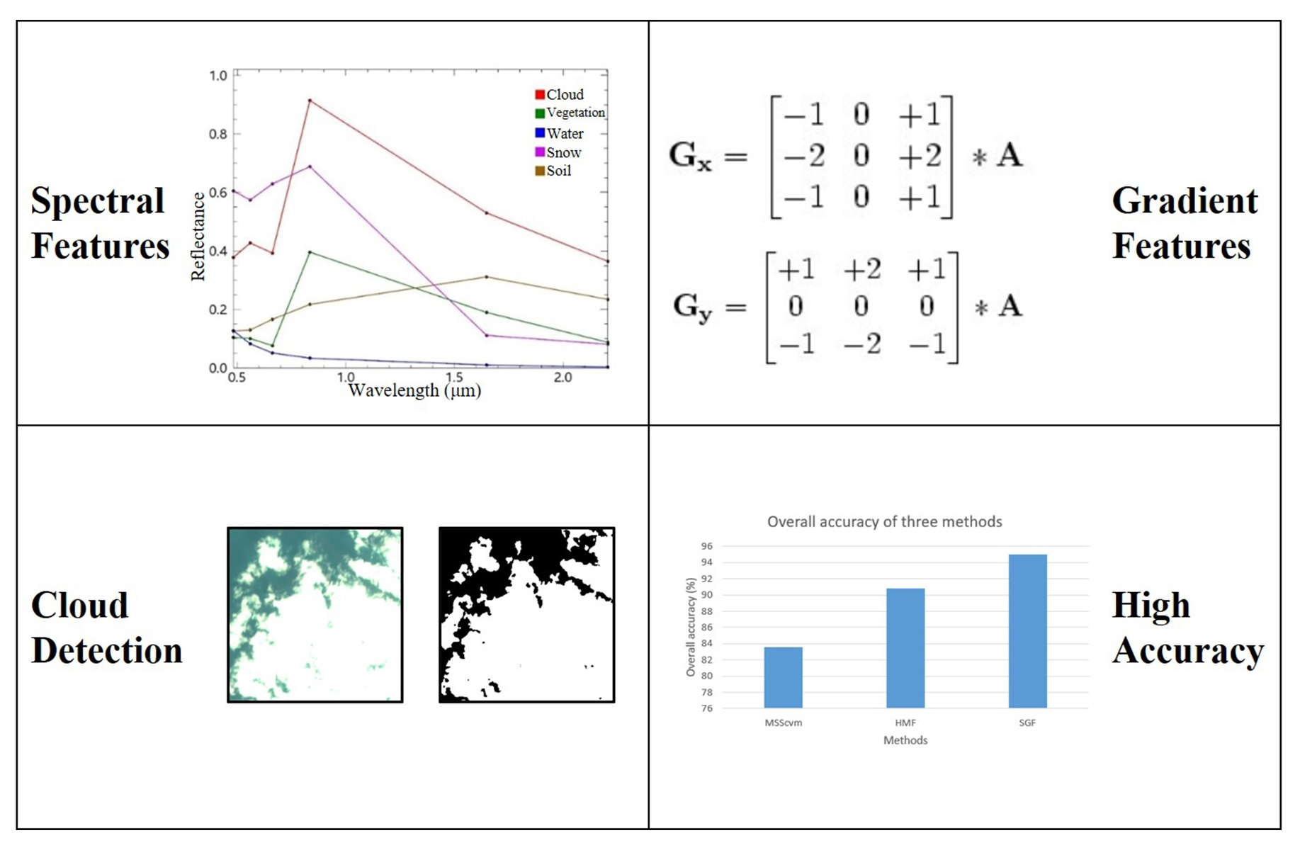
2.2. Spectral Features

In the spectral discriminant, this paper chooses the top of atmosphere (TOA) reflectance as input. TOA reflectance can be calculated based on some parameters, such as gain, bias, Earth–Sun distance and solar irradiancy at the mean Earth–Sun distance [30]. These parameters can be obtained in meta files of each image and some fixed parameters are shown in Table 2.
Due to the bright nature of cloud, TOA reflectance of cloud is high in all the bands, and the brightness can be used as a feature to detect cloud. Analyzing all the bands, this paper finds that TOA reflectance of cloud in band 1 and band 2 is slightly lower than other bands. TOA reflectance of vegetation increases in band 6 and band 7, which lead to misjudgment. Therefore, TOA reflectance of band 3, band 4, and band 5 is adopted. Brightness discriminant is as follows:
M e a n = B 3 + B 4 + B 5 3 > t h r e s h _ M e a n
where, M e a n is average of TOA reflectance, B 3 , B 4 , and B 5 are TOA reflectance of band 3, band 4, and band 5, and t h r e s h _ M e a n is threshold of M e a n .
NDWI proposed by McFeeters [31] is an index to detect water. Because the reflectance of visible bands is slightly higher than that of NIR, NDWI of water is a positive value, while NDWI of cloud is a negative value. From experiments, this paper finds that band 4 can widen NDWI difference between cloud and water, which can improve the accuracy of cloud detection. The NDWI discriminant is as follows:
N D W I = ( B 4 B 7 ) ( B 4 + B 7 ) < t h r e s h _ N D W I
where B 7 is TOA reflectance of band 7, and t h r e s h _ N D W I is threshold of NDWI.
In Figure 1a, a multispectral image of SDGSAT-1 from the East China Sea is shown, where the white area is cloud and the other is water, and NDWI is shown in Figure 1b. It can be seen that cloud and water are roughly divided with NDWI by 0, which is an obvious difference between cloud and water; therefore, NDWI can be well applied to the SDGSAT-1.
NDVI is an index to detect vegetation [32]. The reflectance of vegetation is low in visible bands and there is a large increase from the red band to the NIR band, so the NDVI of vegetation is high. While cloud has high reflectance in both the red band and the NIR band, the NDVI of cloud is lower than that of vegetation. Band 5 and band 7 are selected to calculate NDVI. The NDVI discriminant is as follows:
N D V I = ( B 7 B 5 ) ( B 7 + B 5 ) < t h r e s h _ N D V I
In Figure 2a, a multispectral image of SDGSAT-1 from southwestern Siberia is shown, where the white area is cloud and the other is vegetation, and the NDVI is shown in Figure 2b. From Figure 2, there is a difference between the NDVI of cloud and that of vegetation. There is also the NDVI of thin cloud which lies in between thick cloud and vegetation, and the thin cloud can also be detected using dynamic thresholds. Therefore, cloud and vegetation can be distinguished with NDVI.
Because the observation time, solar zenith angle, and local environment of each image are different, the reflectance of the same ground objects in different images is also different. Compared with the fixed thresholds which cannot be adapted to each image, dynamic thresholds have an excellent advantage. Otsu’s method is a simple and efficient image segmentation algorithm and has good performance. It divides images into foreground and background based on gray-scale values. When the best threshold is selected, the maximum variance between clusters is the largest. Therefore, t h r e s h _ M e a n , t h r e s h _ N D W I , and t h r e s h _ N D V I are obtained with Otsu’s method, which can improve cloud detection accuracy. From the above analysis, there is a large difference between cloud and other ground objects, and thresholds can be obtained quickly and efficiently with Otsu’s method.
HOT, proposed by Zhang et al. [33], is based on the idea that the visible bands for most ground objects are highly correlated, but the spectral response to cloud is different between the blue and red wavelengths. It can be used in detecting cloud, especially thin cloud. HOT was also used in cloud detection by Vermote et al. [34] and Zhu et al. [21] for Landsat 7, and results were successful. However, each band reflectance of SDGSAT-1 is lower than that of Landsat 7. Therefore, after experiments, parameters are changed to adapt to SDGSAT-1. The HOT discriminant is as follows:
H O T = B 3 0.5 × B 5 0.06 > 0
After the above detection with spectral features, most ground objects have been removed and cloud-like pixels are obtained. However, cloud-like may include snow that is mistakenly detected as cloud. The method of how to distinguish cloud and snow will be introduced in the next section.

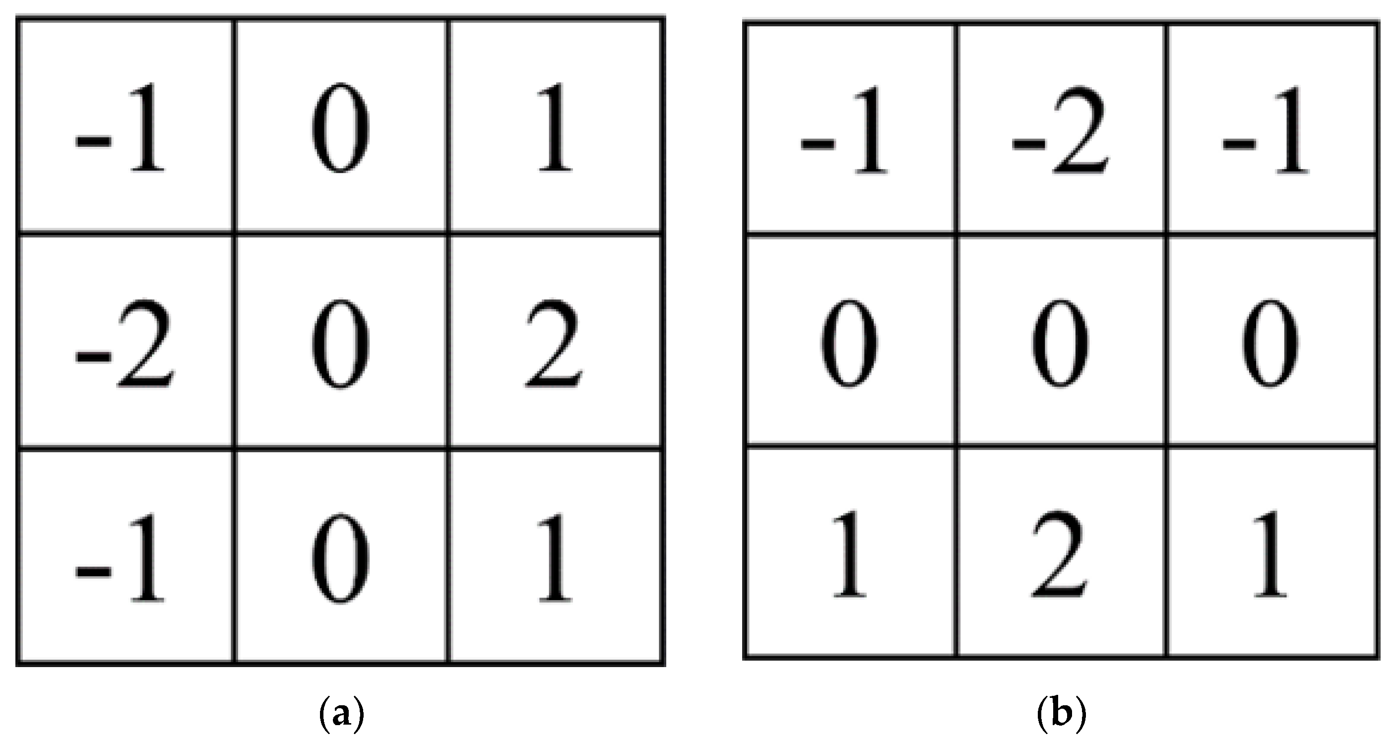
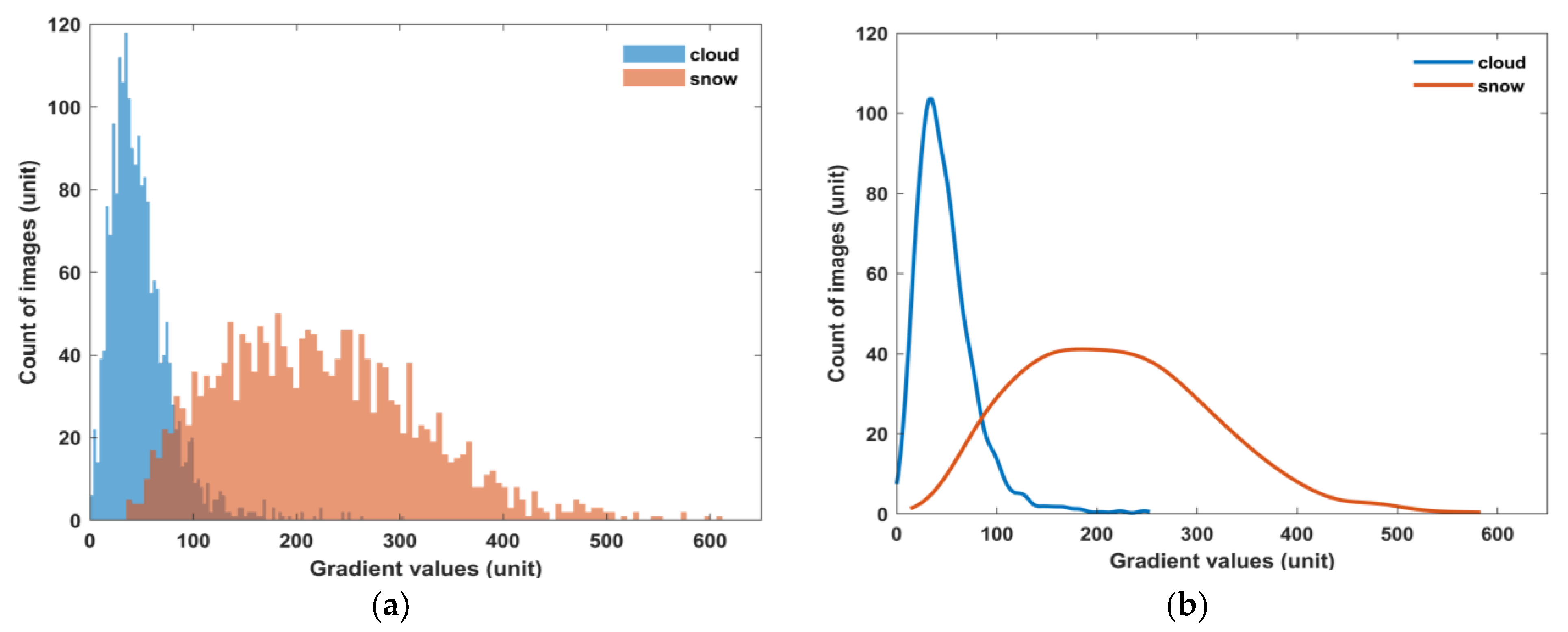
2.3. Gradient Features

The spectral features of snow are similar to that of cloud. For example, cloud and snow have a bright nature, so the reflectance of them is high in many bands. Due to the similar spectral features, cloud and snow are difficult to be distinguished. In cloud detection, how to remove snow is a long-standing problem. Due to the lack of the SWIR band in SDGSAT-1 MII, NDSI cannot be adopted. Therefore, this paper finds other methods to distinguish cloud and snow.
Although cloud and snow are similar in spectral features, there are some differences in gradient features [35]. The images of cloud and snow in band 5 are shown in Figure 3. From Figure 3a, the gray values of the cloud center are large, and that of the thin cloud at the boundary is small. In addition, the gray values of cloud decrease gradually from the center to the boundary, and the edges of the cloud are smooth. It can be seen from Figure 3b that the central area of snow is similar to cloud with large gray values, but the boundary between bright (snow) and dark (no snow) areas is sharper.
The degree of sharpness can be represented by the gradient. The sharper the edge, the larger the gradient. Because digital images are discrete, the gradient is usually represented by first-order difference. The Sobel operator is used in this paper, which is an edge detection operator based on first-order difference. It has the advantages of obtaining gradient in the diagonal direction and suppressing noise [36].
The Sobel operator convolution kernel is shown in Figure 4. The weighted average of the gray-scale values for the 8 connected neighborhoods of each pixel f(x,y) is determined, and the gradient in the x and y directions of the pixel are as follows:
{ g x = f ( x + 1 , y 1 ) + 2 f ( x + 1 , y ) + f ( x + 1 , y + 1 ) f ( x 1 , y 1 ) 2 f ( x 1 , y ) f ( x 1 , y + 1 ) g y = f ( x 1 , y + 1 ) + 2 f ( x , y + 1 ) + f ( x + 1 , y + 1 ) f ( x 1 , y 1 ) 2 f ( x , y 1 ) f ( x + 1 , y 1 )
In image processing, in order to improve computational efficiency, the gradient is as follows:
G = | g x | + | g y |
Band 5 images with the largest contrast are used in gradient calculation in this paper. Firstly, to enhance the contrast of the images and details of ground object edges, histogram equalization for band 5 images is performed. It changes the gray histogram of the original images from a concentrated gray interval to a uniform distribution in the whole gray range. In addition, using a function, the edge detection of cloud-like pixels is performed and edges are obtained. Finally, the gradient average of each cloud-like pixel area is calculated and the threshold judgment is performed; then, cloud pixels are obtained.
In order to obtain the gradient threshold, this paper separately selects some images with cloud and snow, then counts the gradient average of cloud and snow. The histogram of the gradient average of cloud and snow is shown in Figure 5a. From Figure 5a, it can be seen that the gradient average of cloud mainly lies between 0 and 100, and only a few clouds have gradient average above 100. However, the gradient average of most snow is much larger than that of cloud, which mainly lies between 100 and 400, and some are even above 400. This experiment shows that the gradient average of cloud is quite different from that of snow. Although the histogram of cloud and snow have overlapping areas, cloud and snow can be distinguished as much as possible. In Figure 5b, the graph obtained by fitting the histogram of gradient average is shown. From Figure 5b, the intersection of the two curves can be used as the gradient threshold. The gradient discriminant is as follows:
g r a d i e n t < t h r e s h _ g r a d i e n t
where t h r e s h _ g r a d i e n t is the threshold of the gradient.
In order to verify whether snow can be detected with gradient features, this paper selects images with cloud and snow to test. Cloud and snow are difficult to distinguish by the human eye and also based on the spectral features of SDGSAT-1 data. Therefore, the snow flag in the quality assurance band (QA) of Landsat-8 images [37] from the same area is used to distinguish cloud and snow. A multispectral image of SDGSAT-1 from western Norway is shown in Figure 6a, and a Landsat-8 image is shown in Figure 6c. From the QA band of the local zoomed image, it can be known that the white area on the left is cloud and that on the right is snow in Figure 6a. The result of snow detection is shown in Figure 6b, where the white area is snow pixels using the gradient discriminant. It can be seen that most of the snow is successfully detected, and clouds are not mistakenly identified as snow. Therefore, cloud and snow can be effectively distinguished with gradient features, which solves the difficult problem of cloud detection for SDGSAT-1 multispectral images.
There is a problem in gradient discrimination. Due to the overlapping areas of cloud and snow in gradient histogram, a small part of cloud is missing by gradient discrimination for images without snow. Therefore, it is necessary to detect whether there is snow in images before performing gradient discrimination. From Figure 5, it can be seen that the gradient of some snow is larger than 400, while the gradient of cloud is lower than 400. So the gradient of the cloud-like pixels is counted. For each SDGSAT-1 multispectral image, if there are many cloud-like pixels with a gradient above 400, the gradient discrimination will be performed. Otherwise, cloud-like pixels are considered as cloud pixels.
In remote sensing images, cloud areas usually contain multiple pixels. In order to eliminate the influence of bright and small ground objects in images, a filter that removes areas less than 5 pixels is used.
The flowchart of the cloud detection method based on spectral and gradient features is shown as Figure 7. Firstly, TOA reflectance is obtained after preprocessing. In addition, brightness, NDWI, NDVI, and HOT are combined to remove most ground objects with Otsu’s method and cloud-like pixels are obtained, which may contain snow pixels mistakenly identified. Then, snow detection is performed; if there is snow in the image, histogram equalization and edge detection are used on cloud-like pixels. After gradient discriminant, cloud pixels are obtained.

3. Results

3.1. Comparison Experiments with Other Methods

In this section, in order to verify the cloud detection performance of SGF in this paper for SDGSAT-1 multispectral images, the results are shown and compared with multispectral scanner clear-view-mask (MSScvm) [38] and hybrid multispectral features (HMF) [39]. MSScvm is a cloud detection method for the MSS sensor of Landsat, which only uses red and green bands and has good performance. HMF is proposed for Gaofen-1 (GF-1) satellite, which uses three spectral threshold combinations and dynamic thresholds calculated according to solar altitude angle. There are few cloud detection methods for SDGSAT-1, and bands of MSS and GF-1 satellite are similar to that of SDGSAT-1 MII. Therefore, SGF is compared with MSScvm and HMF applied to SDGSAT-1 multispectral images.
Images shown in this section are public SDGSAT-1 multispectral images. Due to excessive pixels in images, a part of the images are selected to show. Meanwhile, in order to verify the performance of SGF in different environments, various underlying surface images are selected, such as vegetation, water, snow, and barren surface. Image information is shown in Table 3.
In Figure 8, cloud detection results for an image from southwestern Siberia are shown. It can be seen that three methods exhibit good cloud detection performance. However, from local images, their detection performance for thin cloud is different. Reflectance of thin cloud is affected by underlying surfaces, but the thresholds of MSScvm are fixed. Therefore, the thin clouds marked with red circles are missing, and detection performance for thin cloud is the poorest. Both SGF and HMF use dynamic thresholds, so detection ability for thin cloud is stronger. From local images, SGF detects more thin clouds than HMF at the same position. Therefore, performance of SGF is better than the MSScvm and HMF.
In Figure 9, cloud detection results for an image with snow surface from western Norway are shown. In Figure 9a, the white area in the bottom left is cloud and the white area on the right is snow. It can be seen that MSScvm and HMF misjudge snow on the right as cloud. This is because the SWIR band is not used in them. The spectral reflectance of cloud and snow are similar in all bands, so MSScvm and HMF cannot distinguish cloud and snow. From Figure 9d, snow is almost removed, and cloud is successfully detected, so SGF has powerful performance for distinguishing cloud and snow. This is because SGF uses gradient features to remove snow, in addition to spectral features, which solves the difficulty of distinguishing cloud and snow for SDGSAT-1 multispectral images.
In Figure 10, cloud detection results for an image from eastern Kazakhstan are shown. MSScvm misjudges a barren surface with high reflectance as cloud because some barren areas have high reflectance in red and green bands, which is similar to cloud. However, HOT is used in SGF and HMF and they have good performance for barren surface detection. Cloud detection results for images from the Yellow Sea and northwestern Canada are shown as Figure 11 and Figure 12. It can be seen that the three methods have good performance for vegetation and water surfaces.
In summary, MSScvm is a method with only two band combinations so it has poor performance for images with barren and snow surfaces. HMF adopts HOT, so the ability for thin clouds and barren surfaces is better. In SGF, four spectral combinations are used in distinguishing most ground objects and thin cloud, and gradient features are used in distinguishing cloud and snow. Therefore, SGF has excellent performance for SDGSAT-1 multispectral images.

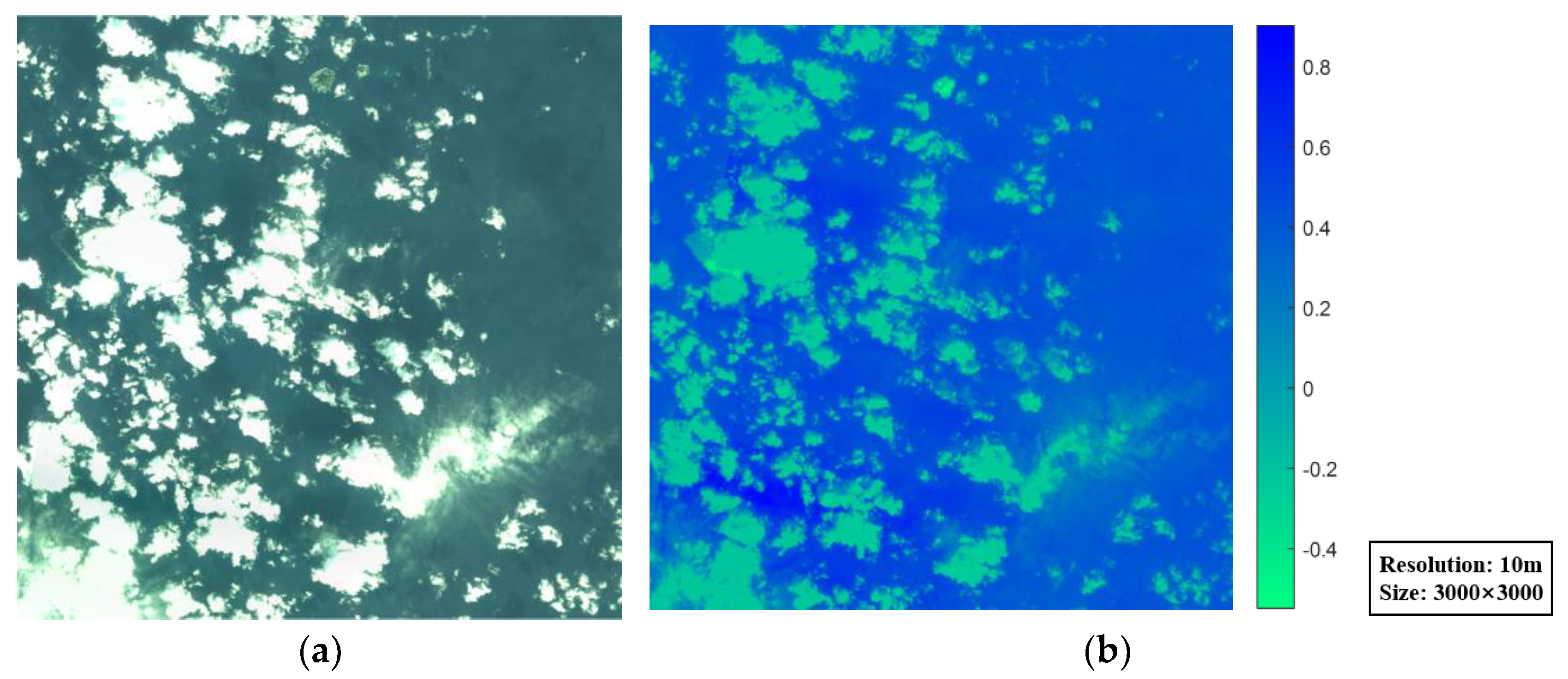
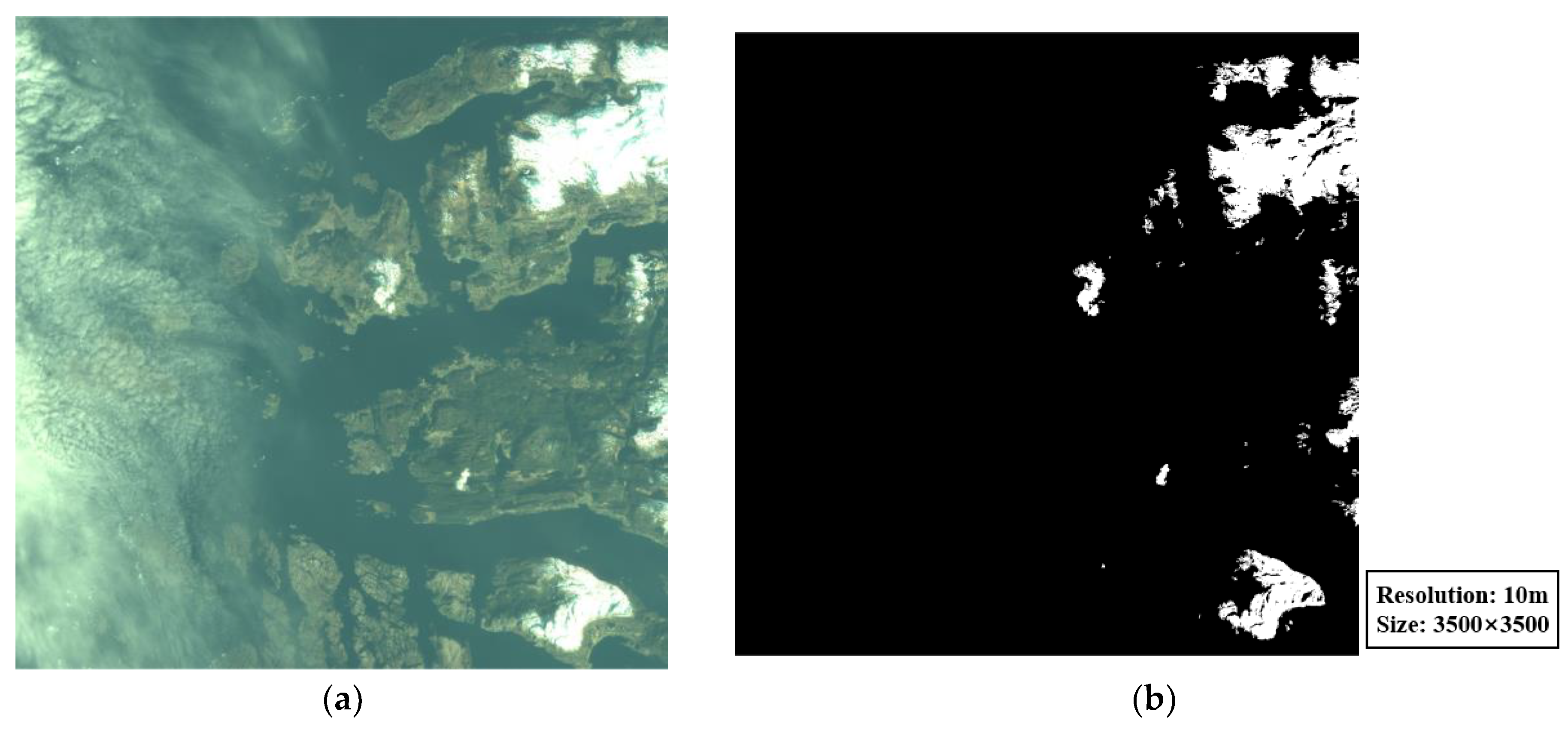
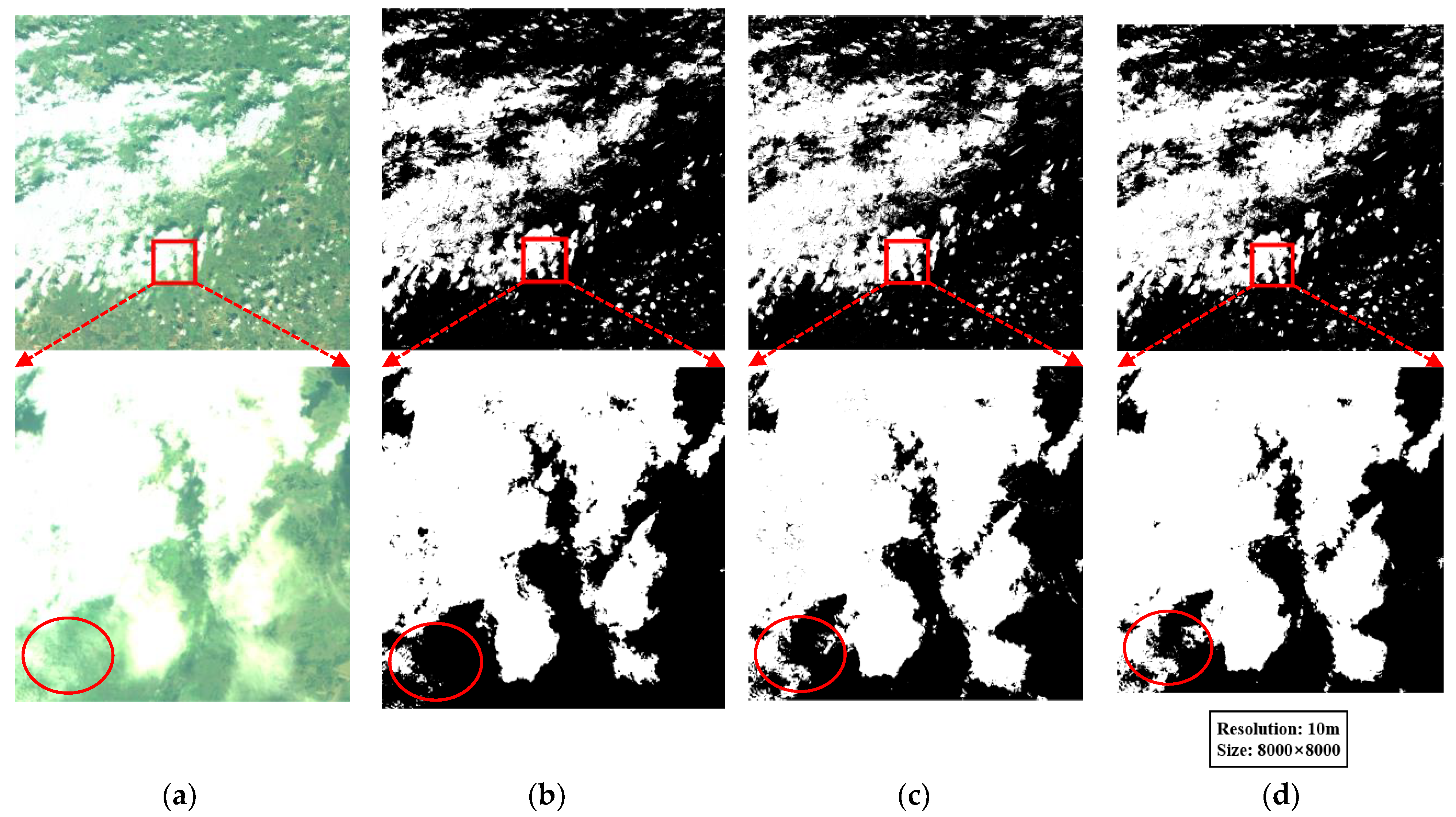
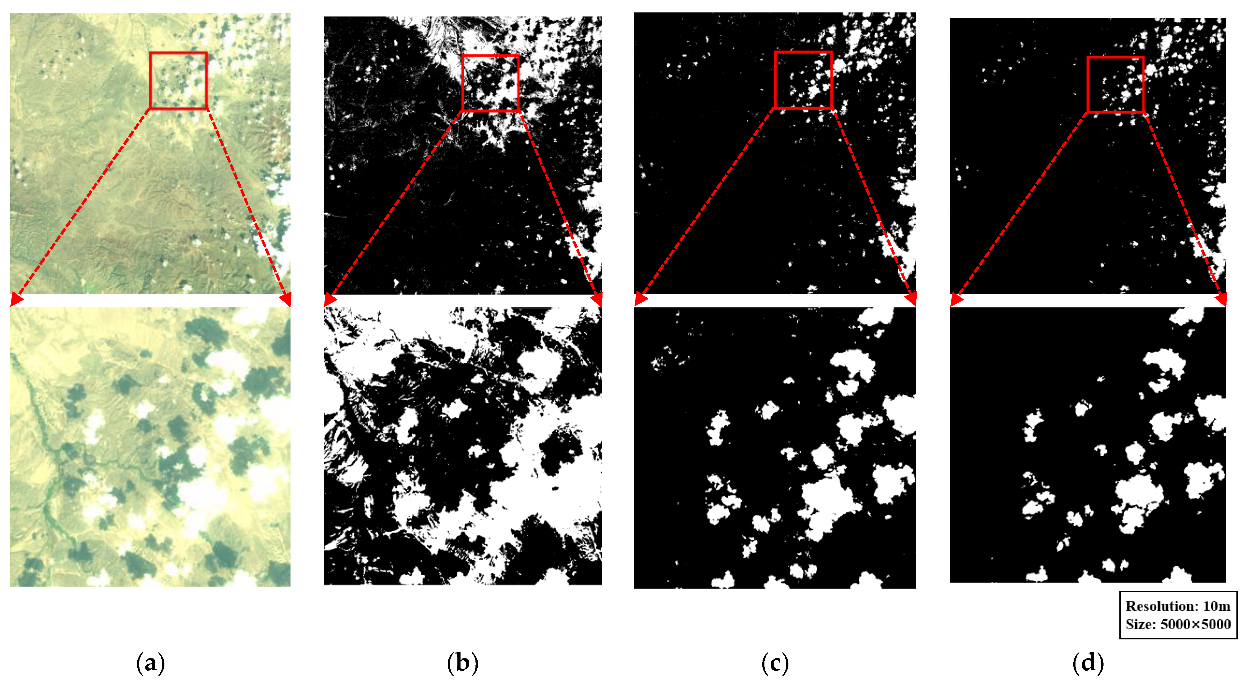
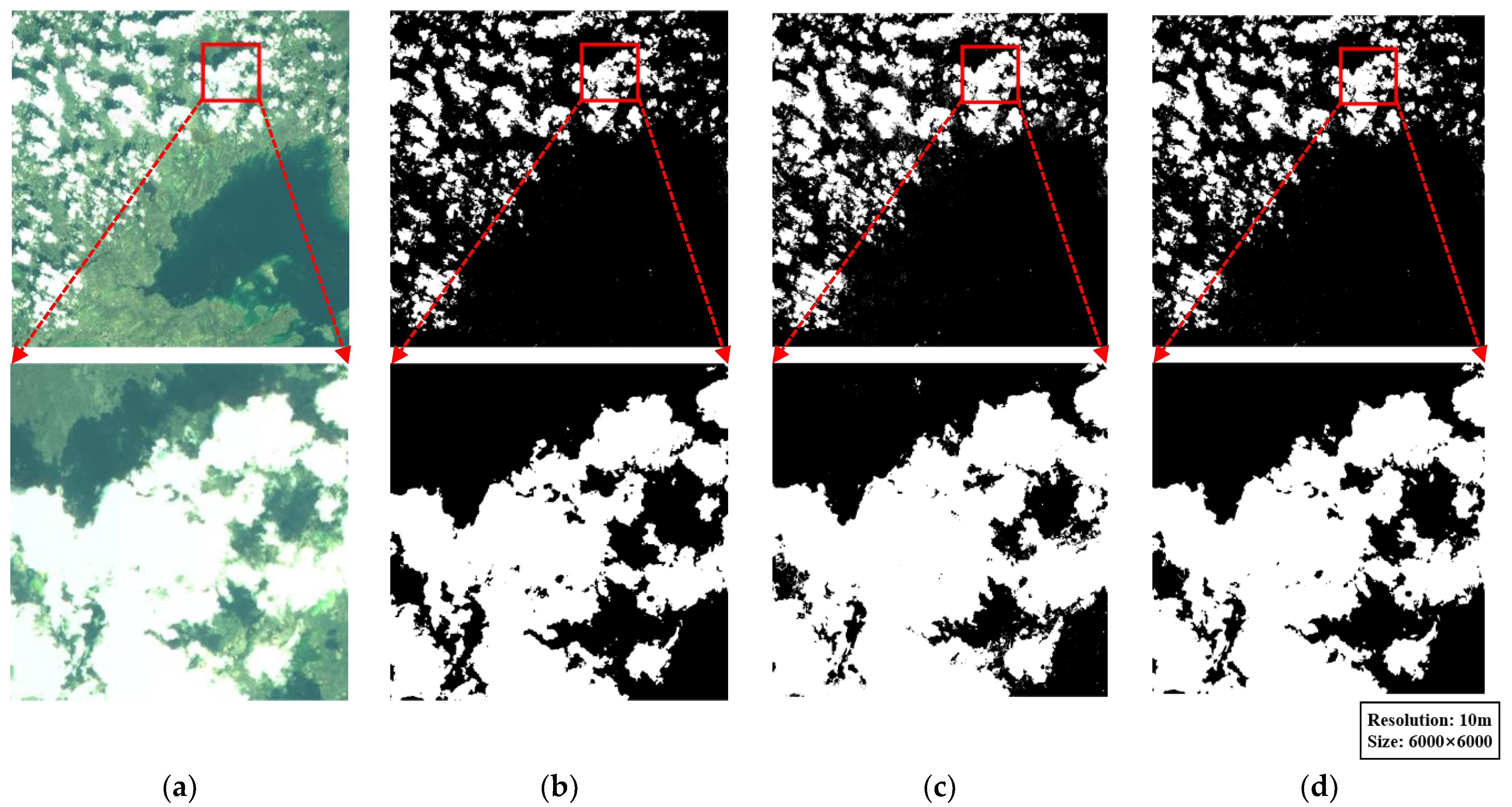
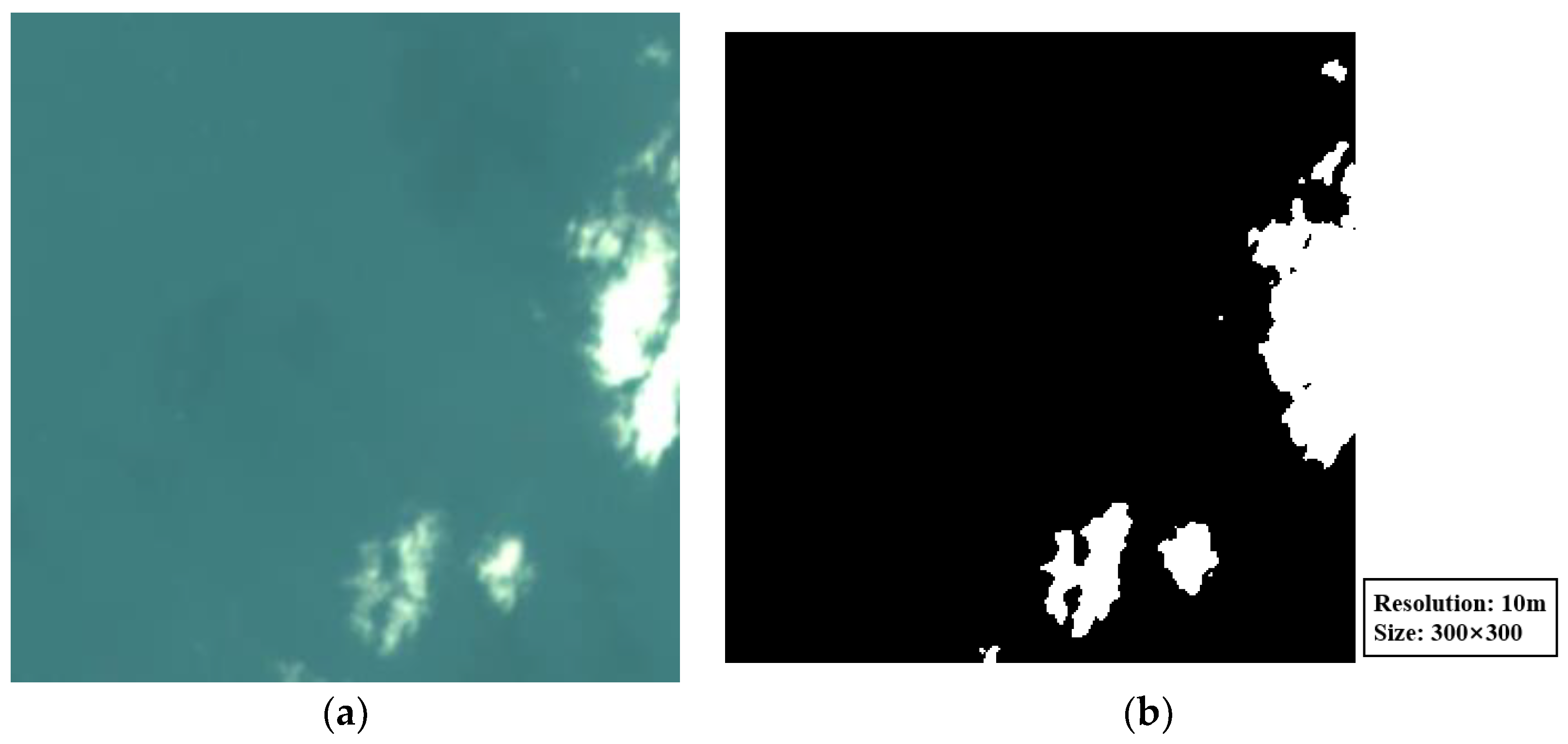
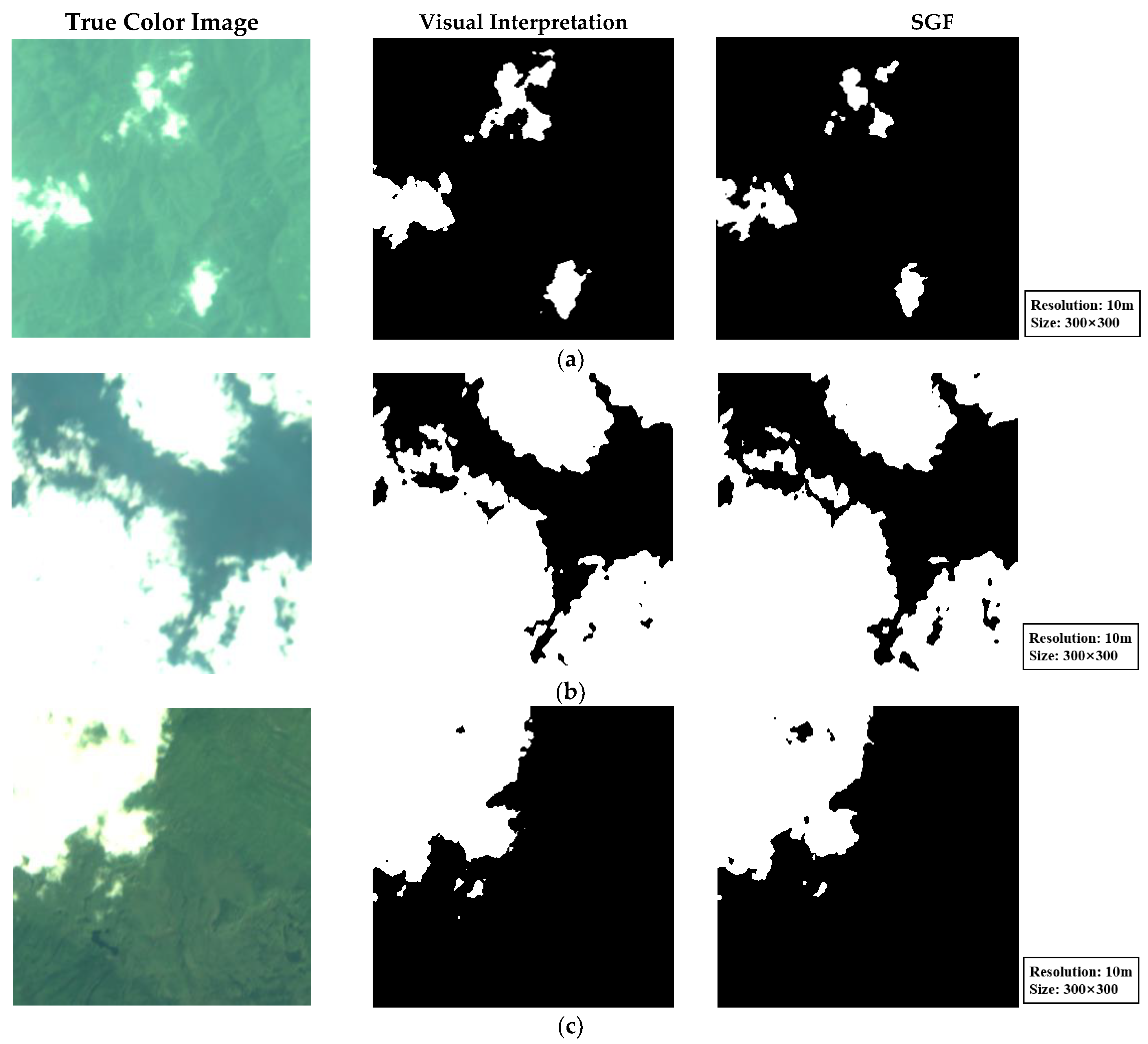
3.2. Visual Interpretation

To evaluate cloud detection accuracy, the real cloud pixels of SDGSAT-1 images need to be obtained and then they can be compared with the cloud detection results. There is no QA band in the SDGSAT-1 images, so the paper combines manual techniques and the QA band of Landsat-8 Level-1 products with similar time and the same area to recognize real cloud pixels. Due to the high reflectance of cloud, a threshold is used and most of the real cloud pixels are obtained. However, some thin cloud around thick cloud has a lower reflectance and may be missing. So we also used manual judgments to recognize the missing cloud.
In addition, the reflectance of snow is similar to that of cloud, so cloud and snow may not be distinguished correctly by the human eye. The paper selects the QA band of Landsat-8 Level-1 products with similar time and the same area to solve this question. Snow pixels are identified by the snow flag in the QA band, so they can be removed from real cloud pixels according to the comparison of SDGSAT-1 images and Landsat-8 images in the same area. Meanwhile, the position of cloud changes quickly, but the position of snow changes slowly. Therefore, cloud can be identified by the contrast of position. Through visual interpretation, the real cloud pixels of SDGSAT-1 images can be obtained. An image and the visual interpretation results are shown as Figure 13. It can be seen that the real cloud pixels are identified.

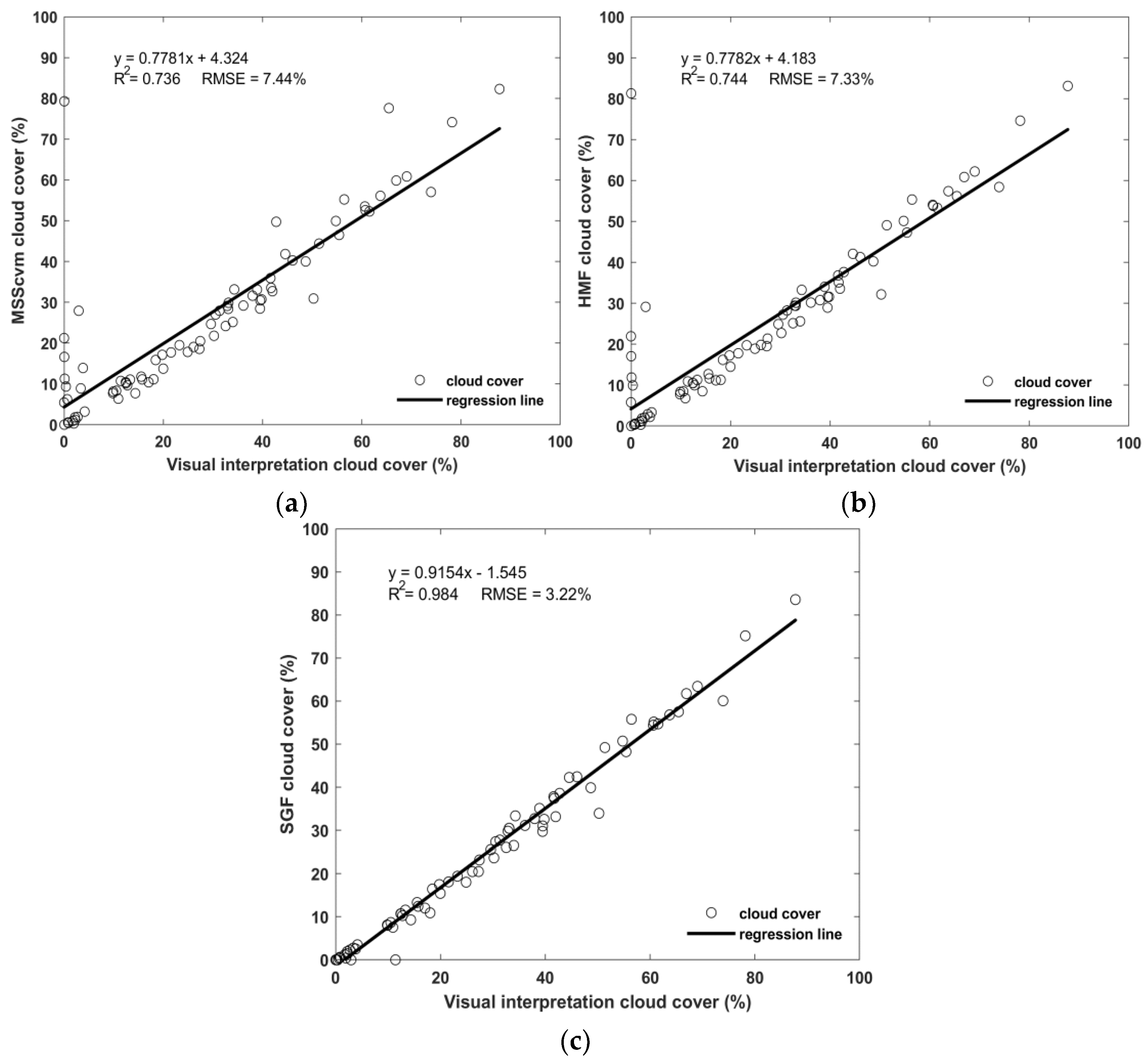
3.3. Accuracy Evaluation

In order to quantitatively evaluate the cloud detection performance of three methods, this paper uses the overall accuracy as the evaluation index [40]. Cloud detection results are compared with visual interpretation results, and overall accuracy of the method is obtained. Due to the large workload of visual interpretation, 300 × 300 pixels in images are randomly selected for visual interpretation, which are compared with cloud detection results. The calculation formula of overall accuracy is as follows:
overall   accuracy = T P + T N N
where T P is the number of cloud pixels that are correctly identified cloud pixels, T N is the number of non-cloud pixels that are correctly identified non-cloud pixels, and N is the total number of image pixels.
SGF overall accuracy based on 85 areas (300 × 300 pixels) that are randomly selected from 10 images is shown as Figure 14, and the average of overall accuracy is 95.00%. Part of the visual interpretation and SGF results are shown in Figure 15. Meanwhile, the overall accuracy average of MSScvm is 83.55% and that of HMF is 90.79%. It can be seen that over 90% of the test images have high overall accuracy in Figure 14. Due to some missing thin clouds, cloud detection overall accuracy decreases. In addition, there are still some test images that have overall accuracy lower than 80%. From an analysis of these test images, this paper finds that the surface of these images is snow. Due to the overlapping areas of cloud and snow in the gradient histogram, some clouds that have a gradient larger than the threshold are mistakenly identified as snow. However, there are also images with snow surface that have an overall accuracy more than 90%, which shows that gradient discriminant has excellent performance for distinguishing cloud and snow.
Comparison of cloud cover between cloud detection methods and visual interpretation is shown in Figure 16. With the linear fit of cloud cover between SGF and true values, the error of SGF can be obtained. It can be seen that the R-square is 0.984, and the root mean square error (RMSE) is 3.22%, which shows that cloud cover of SGF is close to true values and SGF has excellent performance. The R-square of MSScvm and HMF is lower than that of SGF, and the RMSE of MSScvm and HMF is higher than that of SGF, so the performance of SGF is better than that of MSScvm and HMF.
In order to verify cloud detection performance of three methods for different surfaces, images with vegetation, snow, barren, and water surfaces are selected in this section, and over five images for each surface are selected. A total of 20 areas (300 × 300 pixels) in each image were selected to verify. The overall accuracy of cloud detection methods is shown in Table 4.
From cloud detection results and Table 4, MSScvm is only good at cloud detection for vegetation and water surfaces and the overall accuracy is above 93%, while the overall accuracy is only 67.44% and 70.54% for snow and barren surfaces. Because the number of threshold combinations is small, it is difficult to identify ground objects with similar spectral features to cloud. Due to the addition of HOT, HMF can effectively detect cloud with barren surface, and the overall accuracy reaches 93.06%. However, it is also difficult to distinguish cloud and snow. The overall accuracy is only 77.48% for snow surface, which is higher than MSScvm due to the stronger thin cloud detection. Compared with the other two methods, SGF has outstanding advantages in cloud detection for snow surface. Due to the addition of the gradient discrimination, the performance of distinguishing cloud and snow is greatly improved. The overall accuracy for snow surface reaches 90.80%, which is much higher than MSScvm and HMF and can meet the accuracy requirements of cloud mask products. Meanwhile, the stability and accuracy of SGF are improved due to dynamic thresholds, the overall accuracy for other surfaces of SGF is above 94%, which is also higher than MSScvm and HMF.

4. Discussion

SDGSAT-1 can observe global regions and the environment and climate around the world are complex. In order to adapt to images of different regions and improve cloud detection performance, dynamic thresholds are used in the method proposed in this paper. From experimental results, it can be seen that this method has excellent accuracy for images with different surfaces, and the robustness is improved for the subsequent engineering applications. In addition, it is difficult to distinguish cloud and snow with spectral features. Therefore, this paper analyzes gradient features and discusses the difference of the edge gradient between cloud and snow. Then, according to the gradient threshold, cloud and snow are successfully distinguished.
However, there is still a certain error in the cloud detection results: (1) The gradient of cloud and snow have overlapping areas in the gradient histogram, which means that there is a certain error in gradient discrimination. (2) If there is no snow in the image and gradient discrimination is still performed, a small part of cloud will be missing. Therefore, before gradient discrimination, the cloud-like pixels are detected. If there is no snow in the image, gradient discrimination will not be performed so that missing cloud pixels can be avoided. From results for vegetation, water, and barren surfaces, the cloud detection accuracy does not decrease. (3) Gradient features are used in distinguishing cloud and snow, which is already a big improvement for SDGSAT-1. However, there is a situation that cloud and snow overlap. Due to the lack of SWIR band in SDGSAT-1 MII, cloud and snow are difficult to distinguish in this situation. This situation will be studied in our future work. (4) Most thin cloud around thick cloud can be detected by the method, but due to the lack of Cirrus band in SDGSAT-1 MII, some thin cirrus cloud areas are missed. The method of improving thin cloud accuracy will be studied in our future work.

5. Conclusions

In this paper, according to the band characteristics of SDGSAT-1 MII, a cloud detection method based on spectral features and gradient features is proposed for SDGSAT-1 multispectral images. Through the analysis and experiments of spectral features, this paper combines brightness, NDWI, NDVI, and HOT to distinguish cloud and most ground objects. The dynamic threshold using Otsu’s method is adopted to adapt to images with different surfaces and improve the cloud detection accuracy. In addition, this paper finds that the gradient of gray values at the edge of snow areas is larger than that for cloud areas, so the gradient features are used to distinguish cloud and snow.
In experiments, the method proposed in this paper is compared with MSScvm and HMF. Images with different surfaces are selected to verify the cloud detection performance and overall accuracy is used in accuracy evaluation. According to the experiment results, the conclusions are as follows: (1) The method proposed in this paper has excellent performance. The average of overall accuracy reaches 95.00%. From the linear fit of cloud cover between the method and true values, R-square is 0.984 and RMSE is 3.22%. (2) Gradient discriminant can effectively distinguish cloud and snow. It is difficult to remove snow only based on spectral features, so gradient discriminant is proposed in this paper to distinguish cloud and snow, and the overall accuracy for snow surface reaches 90.80%. (3) With the comparison experiments, the overall accuracy for four surfaces is higher than MSScvm and HMF.
The main contributions of this work are as follows: (1) A cloud detection method with excellent performance is proposed for SDGSAT-1 multispectral images. (2) This method solves the difficulty of distinguishing cloud and snow for SDGSAT-1 MII without the SWIR band. (3) Cloud masks and cloud cover can be obtained for subsequent engineering applications. In addition, we will improve snow detection and the dynamic threshold to improve cloud detection accuracy in future works. In addition, images are also contaminated by cloud shadows, so cloud shadow detection will be one of our future works.

Author Contributions

Conceptualization, K.G. and J.L.; methodology, K.G. and J.L.; software, K.G.; validation, K.G., J.L. and F.W.; formal analysis, B.C.; investigation, K.G. and J.L.; resources, K.G., J.L. and F.W.; data curation, K.G. and J.L.; writing—original draft preparation, K.G.; writing—review and editing, J.L., F.W., B.C. and Y.H.; visualization, K.G. and J.L.; supervision, B.C.; project administration, J.L. and F.W.; funding acquisition, Y.H. All authors have read and agreed to the published version of the manuscript.

Funding

This research received no external funding.

Data Availability Statement

The SDGSAT-1 data in this paper are free and can be downloaded from this website: http://124.16.184.48:6008/home (accessed on 1 August 2022).

Conflicts of Interest

The authors declare no conflict of interest.

Abbreviations

The following abbreviations are used in this manuscript.
SDGSAT-1Sustainable Development Science Satellite-1
MIIMulti-spectral imager
SWIRShort-wave infrared
SGFSpectral and gradient features
NDWINormalized difference water index
NDVINormalized difference vegetation index
HOTHaze-optimized transformation
ACCAAutomatic cloud cover assessment
TIRThermal infrared
NIRNear infrared
FmaskFunction of mask
LLLLow-light-level imager
TISThermal infrared spectrometer
NDSINormalized difference snow index
TOATop of atmosphere
QAQuality assurance
MSScvmMultispectral scanner clear-view mask
HMFHybrid multispectral features

References

  1. Nguyen, T.T.; Hoang, T.D.; Pham, M.T.; Vu, T.T.; Nguyen, T.H.; Huynh, Q.-T.; Jo, J. Monitoring Agriculture Areas with Satellite Images and Deep Learning. Appl. Soft Comput. 2020, 95, 106565. [Google Scholar] [CrossRef]
  2. Weiss, M.; Jacob, F.; Duveiller, G. Remote Sensing for Agricultural Applications: A Meta-Review. Remote Sens. Environ. 2020, 236, 111402. [Google Scholar] [CrossRef]
  3. Karthikeyan, L.; Chawla, I.; Mishra, A.K. A Review of Remote Sensing Applications in Agriculture for Food Security: Crop Growth and Yield, Irrigation, and Crop Losses. J. Hydrol. 2020, 586, 124905. [Google Scholar] [CrossRef]
  4. Lv, Z.; Liu, T.; Benediktsson, J.A.; Falco, N. Land Cover Change Detection Techniques: Very-High-Resolution Optical Images: A Review. IEEE Geosci. Remote Sens. Mag. 2022, 10, 44–63. [Google Scholar] [CrossRef]
  5. Luo, H.; Liu, C.; Wu, C.; Guo, X. Urban Change Detection Based on Dempster–Shafer Theory for Multitemporal Very High-Resolution Imagery. Remote Sens. 2018, 10, 980. [Google Scholar] [CrossRef] [Green Version]
  6. Zellweger, F.; De Frenne, P.; Lenoir, J.; Rocchini, D.; Coomes, D. Advances in Microclimate Ecology Arising from Remote Sensing. Trends Ecol. Evol. 2019, 34, 327–341. [Google Scholar] [CrossRef] [Green Version]
  7. Jiang, L.; Huang, X.; Wang, F.; Liu, Y.; An, P. Method for Evaluating Ecological Vulnerability under Climate Change Based on Remote Sensing: A Case Study. Ecol. Indic. 2018, 85, 479–486. [Google Scholar] [CrossRef]
  8. Lu, X.; Zeng, X.; Xu, Z.; Guan, H. Improving the Accuracy of near Real-Time Seismic Loss Estimation Using Post-Earthquake Remote Sensing Images. Earthq. Spectra 2018, 34, 1219–1245. [Google Scholar] [CrossRef]
  9. Ma, H.; Liu, Y.; Ren, Y.; Yu, J. Detection of Collapsed Buildings in Post-Earthquake Remote Sensing Images Based on the Improved Yolov3. Remote Sens. 2019, 12, 44. [Google Scholar] [CrossRef] [Green Version]
  10. Abdollahi, M.; Islam, T.; Gupta, A.; Hassan, Q. An Advanced Forest Fire Danger Forecasting System: Integration of Remote Sensing and Historical Sources of Ignition Data. Remote Sens. 2018, 10, 923. [Google Scholar] [CrossRef]
  11. Barmpoutis, P.; Papaioannou, P.; Dimitropoulos, K.; Grammalidis, N. A Review on Early Forest Fire Detection Systems Using Optical Remote Sensing. Sensors 2020, 20, 6442. [Google Scholar] [CrossRef] [PubMed]
  12. Meng, X.; Shen, H.; Yuan, Q.; Li, H.; Zhang, L.; Sun, W. Pansharpening for Cloud-Contaminated Very High-Resolution Remote Sensing Images. IEEE Trans. Geosci. Remote Sens. 2019, 57, 2840–2854. [Google Scholar] [CrossRef]
  13. Shen, H.; Wu, J.; Cheng, Q.; Aihemaiti, M.; Zhang, C.; Li, Z. A Spatiotemporal Fusion Based Cloud Removal Method for Remote Sensing Images with Land Cover Changes. IEEE J. Sel. Top. Appl. Earth Obs. Remote Sens. 2019, 12, 862–874. [Google Scholar] [CrossRef]
  14. Birk, R.; Camus, W.; Valenti, E.; McCandless, W. Synthetic Aperture Radar Imaging Systems. IEEE Aerosp. Electron. Syst. Mag. 1995, 10, 15–23. [Google Scholar] [CrossRef]
  15. Guo, H. Big Earth Data: A New Frontier in Earth and Information Sciences. Big Earth Data 2017, 1, 4–20. [Google Scholar] [CrossRef] [Green Version]
  16. Jiang, M.; Li, J.; Shen, H. A Deep Learning-Based Heterogeneous Spatio-Temporal-Spectral Fusion: Sar and Optical Images. In Proceedings of the 2021 IEEE International Geoscience and Remote Sensing Symposium IGARSS, Brussels, Belgium, 11–16 July 2021. [Google Scholar]
  17. Li, X.; Feng, R.; Guan, X.; Shen, H.; Zhang, L. Remote Sensing Image Mosaicking: Achievements and Challenges. IEEE Geosci. Remote Sens. Mag. 2019, 7, 8–22. [Google Scholar] [CrossRef]
  18. Luo, Y.; Guan, K.; Peng, J. Stair: A Generic and Fully-Automated Method to Fuse Multiple Sources of Optical Satellite Data to Generate a High-Resolution, Daily and Cloud-/Gap-Free Surface Reflectance Product. Remote Sens. Environ. 2018, 214, 87–99. [Google Scholar] [CrossRef]
  19. Shen, S.S.; Irish, R.R.; Descour, M.R. Landsat 7 Automatic Cloud Cover Assessment. In Proceedings of the SPIE-The International Society for Optical Engineering AeroSense 2000, Orlando, FL, USA, 24–28 April 2000. [Google Scholar]
  20. Luo, Y.; Trishchenko, A.; Khlopenkov, K. Developing Clear-Sky, Cloud and Cloud Shadow Mask for Producing Clear-Sky Composites at 250-Meter Spatial Resolution for the Seven Modis Land Bands over Canada and North America. Remote Sens. Environ. 2008, 112, 4167–4185. [Google Scholar] [CrossRef]
  21. Zhu, Z.; Woodcock, C.E. Object-Based Cloud and Cloud Shadow Detection in Landsat Imagery. Remote Sens. Environ. 2012, 118, 83–94. [Google Scholar] [CrossRef]
  22. Zhu, Z.; Wang, S.; Woodcock, C.E. Improvement and Expansion of the Fmask Algorithm: Cloud, Cloud Shadow, and Snow Detection for Landsats 4–7, 8, and Sentinel 2 Images. Remote Sens. Environ. 2015, 159, 269–277. [Google Scholar] [CrossRef]
  23. Dong, Z.; Wang, M.; Li, D.; Wang, Y.; Zhang, Z. Cloud Detection Method for High Resolution Remote Sensing Imagery Based on the Spectrum and Texture of Superpixels. Photogramm. Eng. Remote Sens. 2019, 85, 257–268. [Google Scholar] [CrossRef]
  24. Li, P.; Dong, L.; Xiao, H.; Xu, M. A Cloud Image Detection Method Based on Svm Vector Machine. Neurocomputing 2015, 169, 34–42. [Google Scholar] [CrossRef]
  25. Hu, K.; Zhang, D.; Xia, M.; Qian, M.; Chen, B. Lcdnet: Light-Weighted Cloud Detection Network for High-Resolution Remote Sensing Images. IEEE J. Sel. Top. Appl. Earth Obs. Remote Sens. 2022, 15, 4809–4823. [Google Scholar] [CrossRef]
  26. Shao, Z.; Pan, Y.; Diao, C.; Cai, J. Cloud Detection in Remote Sensing Images Based on Multiscale Features-Convolutional Neural Network. IEEE Trans. Geosci. Remote Sens. 2019, 57, 4062–4076. [Google Scholar] [CrossRef]
  27. Otsu, N. A Threshold Selection Method from Gray-Level Histograms. IEEE Trans. Syst. Man Cybern. 1979, 9, 62–66. [Google Scholar] [CrossRef] [Green Version]
  28. Salomonson, V.V.; Appel, I. Estimating Fractional Snow Cover from Modis Using the Normalized Difference Snow Index. Remote Sens. Environ. 2004, 89, 351–360. [Google Scholar] [CrossRef]
  29. Warren, S.G. Optical Properties of Ice and Snow. Philos. Trans. A Math Phys. Eng. Sci. 2019, 377, 20180161. [Google Scholar] [CrossRef]
  30. Lu, M.; Li, F.; Zhan, B.; Li, H.; Yang, X.; Lu, X.; Xiao, H. An Improved Cloud Detection Method for Gf-4 Imagery. Remote Sens. 2020, 12, 1525. [Google Scholar] [CrossRef]
  31. McFeeters, S.K. The Use of the Normalized Difference Water Index (Ndwi) in the Delineation of Open Water Features. Int. J. Remote Sens. 1996, 17, 1425–1432. [Google Scholar] [CrossRef]
  32. Carlson, T.N.; Ripley, D.A. On the Relation between Ndvi, Fractional Vegetation Cover, and Leaf Area Index. Remote Sens. Environ. 1997, 62, 241–252. [Google Scholar] [CrossRef]
  33. Zhang, Y.; Guindon, B.; Cihlar, J. An Image Transform to Characterize and Compensate for Spatial Variations in Thin Cloud Contamination of Landsat Images. Remote Sens. Environ. 2002, 82, 173–187. [Google Scholar] [CrossRef]
  34. Vermote, E.; Saleous, N. Ledaps Surface Reflectance Product Description; University of Maryland: College Park, MD, USA, 2007. [Google Scholar]
  35. Guo, Q.; Tong, L.; Yao, X.; Wu, Y.; Wan, G. Cd_Hiefnet: Cloud Detection Network Using Haze Optimized Transformation Index and Edge Feature for Optical Remote Sensing Imagery. Remote Sens. 2022, 14, 3701. [Google Scholar] [CrossRef]
  36. Deng, C.; Ma, W.; Yin, Y. An Edge Detection Approach of Image Fusion Based on Improved Sobel Operator. In Proceedings of the 2011 4th International Congress on Image and Signal Processing, Shanghai, China, 15–17 October 2011. [Google Scholar]
  37. Shen, Y.; Wang, Y.; Lv, H.; Li, H. Removal of Thin Clouds Using Cirrus and Qa Bands of Landsat-8. Photogramm. Eng. Remote Sens. 2015, 81, 721–731. [Google Scholar] [CrossRef]
  38. Braaten, J.D.; Cohen, W.B.; Yang, Z. Automated Cloud and Cloud Shadow Identification in Landsat Mss Imagery for Temperate Ecosystems. Remote Sens. Environ. 2015, 169, 128–138. [Google Scholar] [CrossRef] [Green Version]
  39. Xiong, Q.; Wang, Y.; Liu, D.; Ye, S.; Du, Z.; Liu, W.; Huang, J.; Su, W.; Zhu, D.; Yao, X.; et al. A Cloud Detection Approach Based on Hybrid Multispectral Features with Dynamic Thresholds for Gf-1 Remote Sensing Images. Remote Sens. 2020, 12, 450. [Google Scholar] [CrossRef] [Green Version]
  40. Sun, L.; Mi, X.; Wei, J.; Wang, J.; Tian, X.; Yu, H.; Gan, P. A Cloud Detection Algorithm-Generating Method for Remote Sensing Data at Visible to Short-Wave Infrared Wavelengths. ISPRS J. Photogramm. Remote Sens. 2017, 124, 70–88. [Google Scholar] [CrossRef]
Figure 1. An image from the East China Sea and NDWI (resolution: 10 m; size: 3000 × 3000 pixels): (a) true color image; (b) NDWI.
Remotesensing 15 00024 g001
Figure 2. An image from southwestern Siberia and NDVI (resolution: 10 m; size: 600 × 600 pixels): (a) true color image; (b) NDVI.
Remotesensing 15 00024 g002
Figure 3. Comparison of cloud and snow images from western Norway (resolution: 10 m; size: 40 × 40 pixels): (a) cloud; (b) snow.
Remotesensing 15 00024 g003
Figure 4. Sobel operator convolution kernel: (a) X direction; (b) Y direction.
Remotesensing 15 00024 g004
Figure 5. Gradient average of cloud and snow edges: (a) histogram; (b) fitting graph.
Remotesensing 15 00024 g005
Figure 6. An SDGSAT-1 image from western Norway and snow detection results: (a) true color image of SDGSAT-1 (data: 26 March 2022; resolution: 10 m; size: 3500 × 3500 pixels); (b) snow detection results; (c) an image of Landsat-8 (left); local zoomed image (upper right); snow flag in the QA band of local zoomed image (lower right) (data: 20 March 2022; path: 201; row: 017; resolution: 30 m; Size: 8011 × 8081 pixels).
Remotesensing 15 00024 g006aRemotesensing 15 00024 g006b
Figure 7. The method flowchart.
Remotesensing 15 00024 g007
Figure 8. Cloud detection results for vegetation surface (resolution: 10 m; size: 8000 × 8000 pixels): (a) true color image; (b) MSScvm; (c) HMF; (d) SGF.
Remotesensing 15 00024 g008
Figure 9. Cloud detection results for snow surface (resolution: 10 m; size: 7000 × 7000 pixels): (a) true color image; (b) MSScvm; (c) HMF; (d) SGF.
Remotesensing 15 00024 g009
Figure 10. Cloud detection results for barren surface (resolution: 10 m; size: 5000 × 5000 pixels): (a) true color image; (b) MSScvm; (c) HMF; (d) SGF.
Remotesensing 15 00024 g010
Figure 11. Cloud detection results for water surface (resolution: 10 m; size: 5000 × 5000 pixels): (a) true color image; (b) MSScvm; (c) HMF; (d) SGF.
Remotesensing 15 00024 g011
Figure 12. Cloud detection results for vegetation and water surfaces (resolution: 10 m; size: 6000 × 6000 pixels): (a) true color image; (b) MSScvm; (c) HMF; (d) SGF.
Remotesensing 15 00024 g012
Figure 13. An image from the Indian Ocean and visual interpretation (resolution: 10 m; size: 300 × 300 pixels): (a) true color image; (b) visual interpretation.
Remotesensing 15 00024 g013
Figure 14. Histogram of overall accuracy: (a) MSScvm; (b) HMF; (c) SGF.
Remotesensing 15 00024 g014
Figure 15. Part of visual interpretation and SGF results (resolution: 10 m; size: 300 × 300 pixels): (a) an image from Hunan province; (b) an image from the Indian Ocean; (c) an image from northwestern Canada.
Remotesensing 15 00024 g015
Figure 16. Comparison of cloud cover between cloud detection methods and visual interpretation: (a) MSScvm; (b) HMF; (c) SGF.
Remotesensing 15 00024 g016
Table 1. SDGSAT-1 MII bands.
PayloadBandsTypeWavelength (μm)Resolution (m)
MIIB1Deep blue 10.374–0.42710
B2Deep blue 20.410–0.467
B3Blue0.457–0.529
B4Green0.510–0.597
B5Red0.618–0.696
B6Red edge0.744–0.813
B7Near infrared0.798–0.911
Table 2. Solar irradiancy, gain, and bias of SDGSAT-1 MII.
BandsWavelength (μm)Solar Irradiancy (W/m2/µm)GainBias
B10.374–0.4271532.00.0515601330
B20.410–0.4671893.10.0362413530
B30.457–0.5291978.40.0233168350
B40.510–0.5971883.40.0158496660
B50.618–0.6961613.00.0160963810
B60.744–0.8131224.60.0197190390
B70.798–0.911993.510.0138114580
Table 3. Image information.
SceneDateCenter LongitudeCenter LatitudeSurface
Figure 810 August 202273.5354.88Vegetation
Figure 926 March 20224.2460.82Snow, vegetation, water
Figure 1028 August 202281.3446.27Barren
Figure 118 February 2022123.4236.65Water
Figure 1217 June 2022−118.7964.38Vegetation, water
Table 4. Overall accuracy of cloud detection methods for different surfaces.
SurfaceMSScvmHMFSGF
Vegetation93.93%94.86%95.76%
Snow67.44%77.48%90.80%
Barren70.54%93.06%96.53%
Water94.45%94.51%94.87%
Disclaimer/Publisher’s Note: The statements, opinions and data contained in all publications are solely those of the individual author(s) and contributor(s) and not of MDPI and/or the editor(s). MDPI and/or the editor(s) disclaim responsibility for any injury to people or property resulting from any ideas, methods, instructions or products referred to in the content.

