Article

Dropsonde-Based Heat Fluxes and Mixed Layer Height over the Sea Surface near the Korean Peninsula

1
Observation Research Department, National Institute of Meteorological Sciences, 33, Seohobuk-ro, Seogwipo 63568, Jeju-do, Republic of Korea
2
Department of Environmental Atmospheric Sciences, Pukyong National University, 45, Yongso-Ro, Nam-Gu, Busan 48513, Republic of Korea
*
Author to whom correspondence should be addressed.
Remote Sens. 2023, 15(1), 25; https://doi.org/10.3390/rs15010025
Submission received: 23 October 2022 / Revised: 6 December 2022 / Accepted: 15 December 2022 / Published: 21 December 2022
(This article belongs to the Section Atmospheric Remote Sensing)

Abstract

:
Dropsonde-based sensible heat flux, latent heat flux, and buoyancy flux were estimated over the sea around the Korean Peninsula in 2021. During a preceding severe weather (SW) mission, a total of 243 dropsondes were released from a National Institute of Meteorological Sciences (NIMS) Atmospheric Research Aircraft (NARA). The heat fluxes were indirectly validated by comparison with model-based heat fluxes. The sensible heat flux calculated by the bulk transfer method depended entirely on the temperature difference between the sea level and atmosphere, whereas the latent heat flux was mainly affected by wind speed. Boundary layer heights above 800 m are closely related to buoyancy flux, which is greater in regions with higher sea surface temperatures. Furthermore, the utility of the dropsonde was confirmed in the marine atmospheric boundary layer (MABL) growth, which is difficult to observe in situ and, a relationship was proposed for estimating MABL based on mean meteorological data over the sea level.

1. Introduction

Korea is located in the eastern part of the Eurasian continent, between China and Japan and is protected from the Pacific Ocean by Japan. The three-sided seas of Korea are distinctly affected by regional natural conditions including dynamic oceanographic settings and active mixing by cold and warm currents [1]. The sea is characterized by the Kuroshio currents which transport moisture and heat from the tropics. Oceanic mesoscale such as eddies which act like a biological pump and coastal upwelling are transporting heat budget and water mass and interacting with the atmosphere in the MABL [2,3].
Surface fluxes over the ocean are required to evaluate coupled ocean-atmosphere and weather forecasting models and to provide surface forcing for ocean models. This is useful in understanding the temporal and regional variations in the exchange of heat between the atmosphere and ocean, and provides a large-scale context for field experiments [4]. Ocean-atmosphere heat fluxes are important components of the climate system through which the atmosphere and ocean exchange energy and contribute to maintaining the Earth’s climate system in a state of climate equilibrium. [5]. Ocean heat flux parameters linked to the sea surface temperature (SST) are critical for simulating typhoon structure and intensity [6,7]. Before a typhoon passes through a certain area, the latent and sensible heat fluxes from the warm ocean to the atmosphere supply moisture to the atmosphere [8,9]. The exchange of vapor and heat, consequently caused by the SST, affect heat fluxes and atmospheric boundary layer stability owing to changes in atmospheric fields such as temperature, atmospheric pressure, and wind within the ocean-atmospheric boundary layer [10,11]. For example, a sea heat flux is the amount of heat that evaporates water from the sea surface that results in SST cooling, which is then released to warm the atmosphere when water vapor condenses to form clouds [5]. Sea surface wind can be modified by SST, sea surface currents, and changes in MABL stability.
The heat fluxes can be calculated using the eddy covariance system, which directly estimates the turbulence that exchanges energy and physical quantities between the atmosphere and sea level [12]. However, direct observation of heat flux at sea is limited in space and time because it is performed only at specific points, such as at ships or ocean observation stations [13]. Previous studies have been conducted in which heat fluxes have been calculated by using ship or buoy observation data to the bulk transfer method [14,15,16,17]. Petersen and Renfrew [18] compared the direct heat fluxes (eddy heat fluxes) to the model heat fluxes based on the Coupled Ocean-Atmosphere Response Experiment (COARE) 3.0 algorithm using neutral heat transfer coefficients for moisture and heat. The model-induced heat fluxes were consistently less than the eddy heat fluxes, with a difference of up to 50 W m−2 at times. Bharti et al. [19] reported that heat transfer coefficients over mid-latitudes and strong-wind regimes are still being improved. However, these bulk heat fluxes are not without bias. The model’s input parameters were progressively corrected. They also reported a difference in the buoy-and ship-based heat transfer coefficients. Petersen and Renfrew [20] reported an evident requirement for ocean-atmosphere flux observations. The authors emphasized the importance of eddy heat fluxes over the sea because a lack of direct observations may result in an underestimation of the bulk transfer coefficients and, thus, of model heat fluxes. Fairall et al. [21] stated that sea spray droplet effects are expected to become significant at wind speeds exceeding 15–20 m s−1 and have ignored sea spray droplet effects on the bulk transfer coefficient.
The marine atmospheric boundary layer (MABL) development is strongly related to surface heat fluxes; however identifying MABL over the sea is challenging. Unlike on land where the atmospheric boundary layer height is confirmed by a wind profiler or lidar as well as a radiosonde, MABL has been verified by a radiosonde released from a ship. Aircraft-based observations have some advantages over ship-based observations such as being independent of the sea surface and having more information flow distortion effects for any given run. With the recent development of aircraft-based weather observation technology, data collection by dropsondes, which can determine the vertical profile and height of MABL, is increasing. Zhang et al. [7] estimated the surface flux by applying 2242 Global Positioning System dropsonde observation data to the bulk transfer method. They suggested that sea surface heat fluxes play an important role in strengthening or weakening hurricanes and emphasized the important role of heat flux-based boundary layer recovery in adjusting low-level thermodynamic structures. Bharti et al. [19] calculated bulk heat fluxes using the COARE 3.5 bulk algorithm with in situ data from a ship and used the bulk heat fluxes as in situ heat flux observations to validate model heat fluxes such as Australian Integrated Marine Observing System (IMOS) fluxes, European Centre for Medium-Range Weather Forecasts ReAnalysis-Interim (ERA-Interim) fluxes, and Objectively Analyzed Air-Sea Heat Fluxes (OAFlux).
There remains a lack of a platform capable of directly measuring heat fluxes or estimating MABL over the sea around the Korean Peninsula. The Korea Meteorological Administration (KMA)/NIMS initiated the annual operation of NARA over the sea with the aim of reducing the uncertainty of atmospheric observations as of January 2018 [22]. This study aims to present a method for calculating bulk heat fluxes using a dropsonde and determining the MABL height. We discussed the relationship between SST and heat fluxes. Section 1 describes the development of the MABL based on the dropsonde-based buoyancy flux (BFD) and proposes a method for estimating the MABL height using only simpler measured mean quantities (SST, air temperature, humidity, and wind speed). Section 2 describes the data and a method for estimating the heat fluxes using the bulk transfer method. Section 3 shows dropsonde-based estimates of heat fluxes and verifies the dropsonde-based estimates of heat fluxes with the satellite and model-based heat fluxes. We also suggest a relationship between dropsonde-based estimates of heat fluxes and dropsonde-observed MABL height in Section 4. The conclusions made from these evaluations are given in Section 5.

2. Materials and Method

2.1. Dropsonde

Since 2017, the KMA/NIMS has employed the NARA with the objective of observing for more than 300 h [23]. The NARA used is the Kingair350 from Beechcraft Corporation of the United States, with a maximum operating altitude of approximately 9 km and a maximum operating time of approximately five hours. The NARA observations were conducted in the West Sea (WS), East Sea (ES), and South Seas (SS) of the Korea Air Defense Identification Zone from Gimpo Airport base (Figure 1). The WS is part of the East Asian Marginal Sea, bordering Korea and Japan (north), Taiwan (south), China (west), and the Ryukyu Islands (east). The WS acts as a large reservoir as well as a source and sink of heat energy for transferring the sea to the atmosphere and vice versa [24]. The ES is a semi-enclosed marginal sea that is bounded by the Asian continent, Sakhalin Island, and Japanese islands [25]. Enhancing severe weather (SW) predictability requires aircraft dropsonde data assimilation. The SW predicting mission had four sub-missions: SW-01 (a heavy rain pre-observation mission), SW-02 (a typhoon pre-observation mission), SW-03 (a heavy snow pre-observation mission), and SW-04 (a basic meteorological element comparison of satellite output). The observations for the SW missions were conducted in the areas of WS, ES, and SS. The SW-03 mission was mainly carried out over the ES in the winter, with additional submissions carried out in the WS and the SS. Dropsondes are sensors that measure air temperature (°C), humidity (%), barometric pressure (hPa), and GPS signals to analyze horizontal wind speed (ms−1), wind direction (°). The dropsondes descend at a rate of 11 m s−1 from meteorological aircraft to sea level, thereby providing the aforementioned measurements along the way. Data from Vaisala’s dropsonde (RD-94) data were collected on a NARA using Advanced Vertical Atmospheric Profiling System (UCAR/NCAR, 1993), which receives radio signals transmitted from in-flight dropsondes. The raw data were processed using the Atmospheric Sounding Processing Environment (ASPEN), version 3.3-668, which provides sounding data where provided after applying standard quality control algorithms and corrections [26]. We also compared the dropsonde vertical profile with NARA atmospheric instrument (e.g., AIMMS-20) and confirmed good agreement [22].
Dropsondes were launched from NARA at altitudes ranging from 4 to 9 km in each sea area. In 2021, a total of 49 single day flights were completed, and 243 vertical profiles were obtained (Table 1). Out of which, 115 dropsondes were released from 21 flights during the cyclone period, and 128 dropsondes were released from 28 flights during the anticyclone period. The primary scientific goal of this SW predicting mission was to investigate the atmosphere-ocean interaction for SW [22].

2.2. Sea Surface Temperature

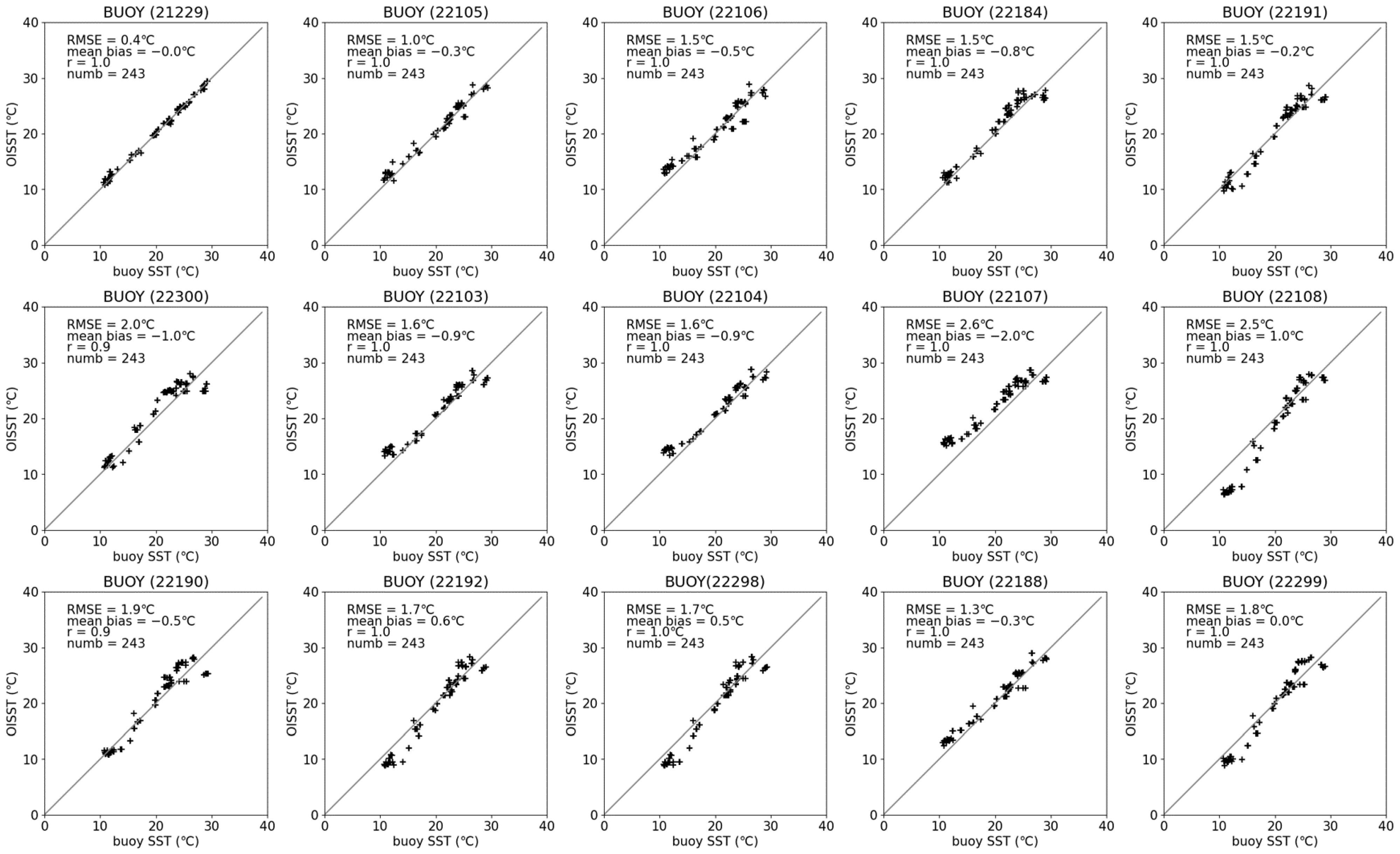
The National Oceanic and Atmospheric Administration (NOAA) provided Optimum Interpolation (OI) SST (v2.1) with a spatial resolution of 0.25° and a temporal resolution of 1 day. The daily mean OISST (from here forward, OISST) was established using a methodology that included bias correction of in situ (ship and buoy) and satellite observations [27,28]. The OISST is based on the combination of both satellite observations from the Advanced Very High Resolution Radiometer (AVHRR), an infrared sensor mounted on NOAA satellite, and in situ observations from ships and buoys. The OISST was compared with the hourly SST measured by 15 KMA marine atmospheric buoys positioned around the Korean Peninsula. Since the KMA buoy data observed by unmanned operating systems may include some anomalous observations, we used in situ measurements obtained after the quality control process [29]. The closest OISST grid data within 0.25° were selected spatially at each buoy point, and the closest buoy SST data were used when the dropsonde observation was performed. The total number of data points used for the comparison was 3810, with a RMSE accuracy of 1.4 °C, a mean bias of −0.3 °C, and a correlation coefficient of 1.0 (Figure 2). When compared with dependent Argo float observations [30], the final v2.1′s mean bias and root mean square error (RMSE) were −0.04 °C and 0.24 °C, respectively [31,32,33]. The mean bias and RMSE are larger than in previous studies due to the different characteristics of the seas around the Korean Peninsula, such as water depth and currents [24,25] and the use of observation data for all four seasons. We assumed that the magnitude of the diurnal fluctuation in sea surface temperature is small and used this as input data for the heat flux calculation alongside dropsonde data.

2.3. Model-Based Heat Fluxes

The model-based sensible heat flux (SHFN) and latent heat flux (LHFN) were provided by the SeaFlux-Climate Data Record (CDR) version 2, which is an ocean surface flux developed with near-surface meteorology derived from passive microwave satellite observations. SeaFlux-CDR version 2 is a significant improvement over SeaFlux-CDR version 1. A novel model-based interpolation approach was used to generate the turbulent heat fluxes and associated values at temporal resolutions of 3-h (01:30, 04:30, 07:30, 10:30, 13:30, 16:30, 19:30, and 22:30 KST, which is the mid-timepoint of each 3-h period in the elapsed-time format from 1988 to the present) and spatial resolution of 0.25°. The dataset is available from the NOAA Climate Data Records repository (https://www.ncei.noaa.gov/products/climate-data-records/ocean-heat-fluxes, accessed on 18 December 2022), which has been widely used in surface energy budget analyses and water cycle research [13,34,35]. We referred to the satellite and model-based sensible heat flux (SHFN) and latent heat flux (LHFN) at the time closest to the launch of each dropsonde (Table 1).

2.4. Bulk Transfer Method

The bulk transfer method was used to calculate the heat fluxes over the sea around the Korean Peninsula. In practical applications, the sensible heat flux and the latent heat flux were estimated directly from the data obtained using eddy covariance equipment using left Equations (1) and (2). The buoyancy flux was estimated using Equation (3) [36]. In addition, it is often related to the mean atmospheric variables via bulk transfer parameterization using right Equations (1) and (2):
SHF = c p ρ a   θ w ¯   c p ρ a C h u 10 ( θ 0 θ 10 )
LHF = L v ρ a   θ w ¯   L v ρ a C q u 10 ( Q 0 Q 10 )
BF = SHF + 0.07 LHF  
where cp (1004 J K−1 kg−1) is the constant pressure-specific heat, L v (2.44 × 10⁶ J kg−1) is the latent heat of vaporization [5,20], and Ch, Cq are the sensible and latent heat transfer coefficients, respectively. ρ a is the atmospheric density of air (1.25 kg m−3),   θ is the fluctuation in air temperature,   w is the fluctuation in vertical wind speed, and the overbar indicates the time-averaged property. θ 0 is the virtual potential temperature (K) at the sea surface and θ 10 is the virtual potential temperature (K) at a reference height (approximately 10 m). Q 0 is the dropsonde-based saturation mixing ratio (g kg−1) closest to sea level using the OISST, and Q 10 is the dropsonde-based mixing ratio (g kg−1) at a reference height (approximately 10 m). u 10 is the dropsonde-based wind speed (m s−1) at the reference height (near 10 m).
The Ch, Cq should be modified regarding the stability of atmospheric conditions to consider the effects of atmospheric stability on the SHF and LHF. This can be achieved by applying dimensionless stability functions [37]. Stability functions ( ψ ) for stable and unstable atmospheric conditions were used in this study. All stability functions for momentum ( ψ m ) , heat ( ψ h ), and moisture ( ψ e ) were assumed to be equal under stable conditions and can be expressed by Equation (4):
0 < z r L ,   ψ m =   ψ h =   ψ e = 5 z r L
The stability functions for momentum ( ψ m ) , heat ( ψ h ), and moisture ( ψ e ) were used under unstable conditions and were expressed as Equation (5):
z r L < 0 ,   ψ m = ln [ ( 1 + x 2 2 ) ( 1 + x 2 ) 2 ] 2 tan 1 x + π 2 z r L < 0 ,   ψ h =   ψ e = 2 ln ( 1 + x 2 2 )  
where x = (1–15 ( z r L ))0.25 [37,38]. Ch, represented by Equation (6), was generally determined before the SHF and LHF can be estimated using Equations (1b) and (2b). The bulk transfer coefficients Ch and Cq for heat and moisture were assumed to be the same [19]. The well-known Monin–Obukhov similarity theory is mostly used to close the bulk transfer parameterization [39,40,41,42]:
C h = k 2 [ ln ( z r z 0 m ) ψ m ( z r L ) ] 1 [ ln ( z r z 0 m ) ψ h ( z r L ) ] 1
C h = C q
where k is the von Karman constant (0.4), zr is the observation reference height (m), and z0m is the roughness length (m). Geernaert et al. [43] used a roughness length of 2.0 × 10⁻⁵ m to calculate the SHF and LHF. Hussein [44] used a roughness length of 7.3 × 10⁻⁴ m to calculate the SHF and LHF. Therefore, according to the surface conditions, we used 1.0 × 10⁻⁴ m as the roughness length over the WS, ES, and SS within the range classified by Stull [43].
u * = ku 10 ln ( z r z 0 m ) ψ m ( z r L )
The Monin–Obukhov length L can be expressed as Equation (8).
L = u * 3 ρ a T av kg [ SHF c p + 0.61 ( T a + 273.16 ) LHF L v ]
where g is the gravitational acceleration (=9.8 m s−2), T av is the virtual air temperature (K) at approximately 10 m, T a is the air temperature (°C) at approximately 10 m, and u * is the friction speed (m s−1) [38,45].
The u * , SHF, and LHF must be estimated to determine L and vice versa. Therefore, L was calculated using an iterative method. When the initial value of L is assumed to be neutral atmospheric stability (=1015), ψ m and ψ h are equal to zero. Based on these variables, u * , Ch, SHF, and LHF can be calculated iteratively using Equations (1)–(8) and substituted into Equation (9) to obtain a new value of L under the condition that the ratio (Ln − Ln−1)/Ln−1 is less than 1% [46,47].

3. Results

3.1. Sea Surface Temperature Field

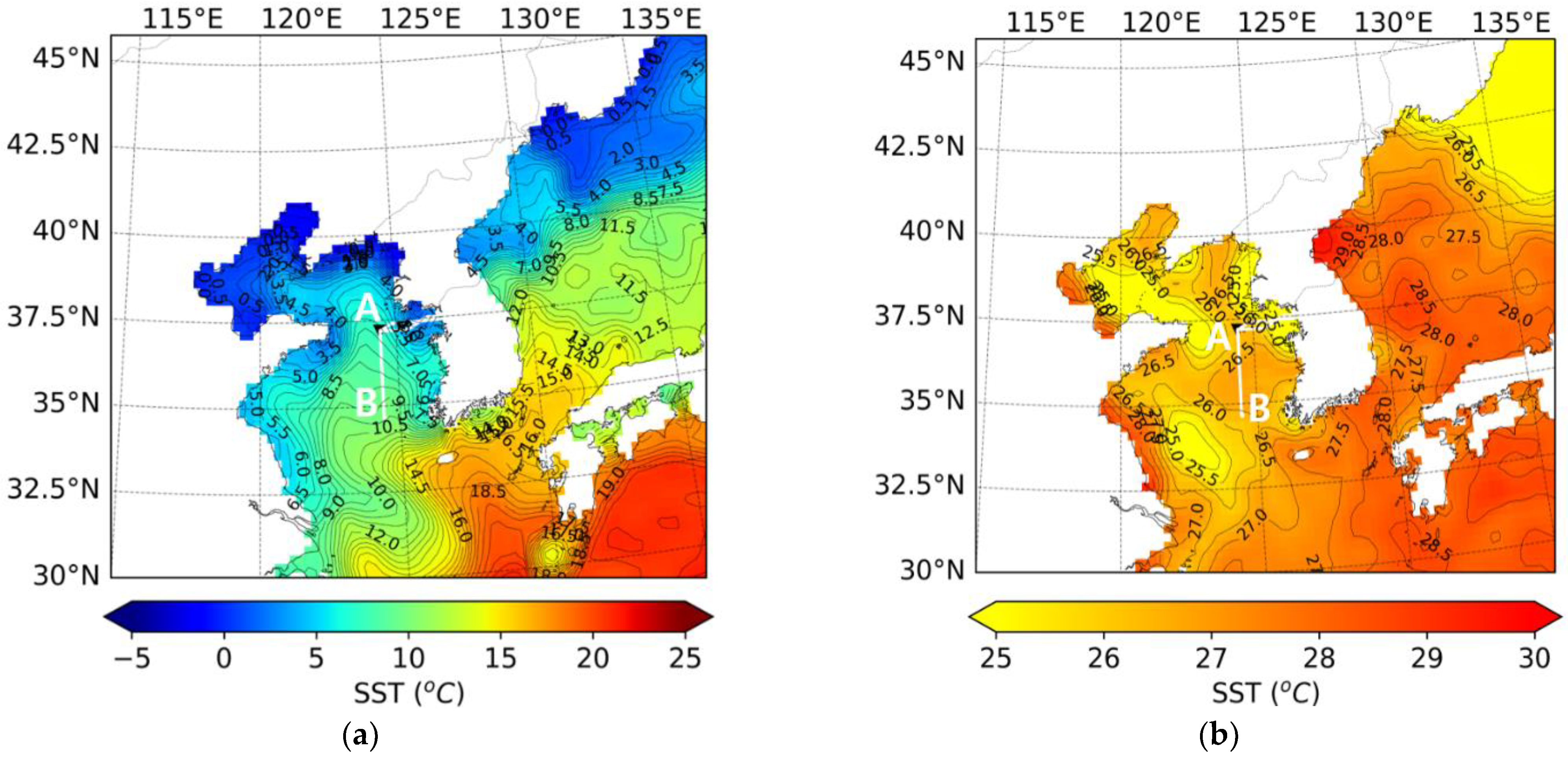
The bulk transfer coefficient, Ch, is influenced by atmospheric stability conditions over the water surface and, as a result, may be affected by the temperature and humidity gradients [20]. Figure 3a,b shows the SST distribution on 3 February (Case 1) and 2 August (Case 2), respectively. Each dropsonde (black triangle) was launched on 37.18°N, 124.43°E and 37.18°N, 124.41°E respectively at an altitude of approximately 4 km in the West Sea (WS). The gradient of SST distribution in winter was greater than the gradient of SST distribution in summer. For each case, the closest SST to where the dropsonde was launched was 7.3 °C and 26.4 °C, respectively.
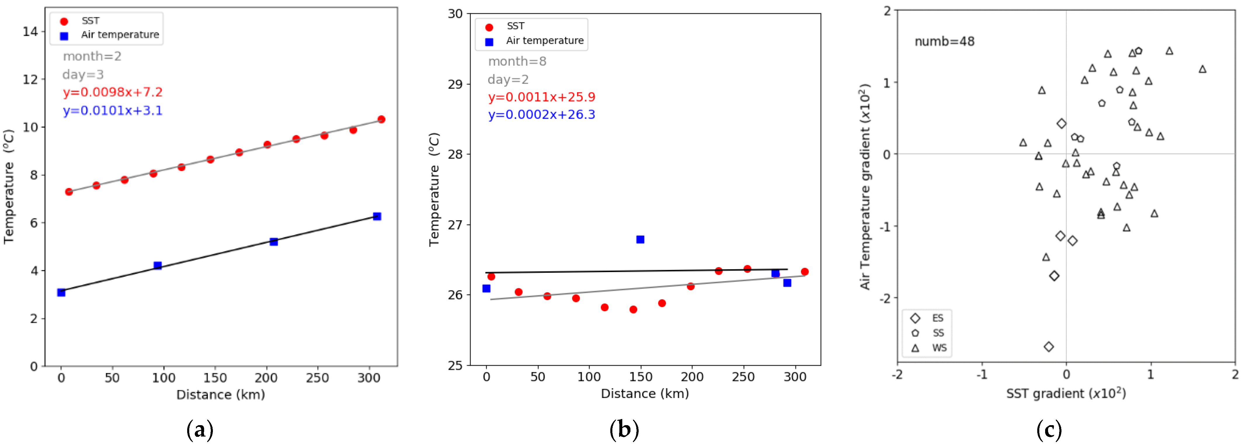
Figure 4a,b shows the SST and dropsonde-based air temperature near 10 m at the point where the dropsonde was launched. In Case 1, both SST and air temperature increased from the initial launch A to the final point B, with SST and air temperature gradients (slope of linear regression) of 0.01 °C km−1. In Case 2, the SST decreased from A to 150 km south and then increased, whereas the air temperature increased and then decreased. This is because the spatial change in water temperature in the shallow West Sea (WS) of the Korea Air Defense Identification Zone was small during summer, hence the SST gradient was not discernible, thus the air temperature gradient could not be obtained.
Figure 4c shows the scatter plot between SST and air temperature gradients in 48 cases (Table 1), except for the 21 January case (because there was only one dropsonde data). The values of SST and air temperature gradient mean the slopes of the linear regression of SST and air temperature in each case. When SST increased, air temperature increased in 29 cases, and when SST decreased, air temperature decreased. When the SST gradient (°C km−1) increased, the air temperature gradient (°C km−1) decreased in four cases, while when it decreased, the temperature gradient increased in 15 cases. In the WS in May, June, and September, the direction of increase and decrease in SST and air temperature did not coincide. This is because the atmosphere was affected by the change in the synoptic scale caused by the approaching cyclone but not by the local sea surface temperature. Kwon et al. [48] reported that during the cyclone period, the MABL structure was primarily affected by synoptic effects, whereas during the anticyclone period, the MABL structure was predominantly affected by local effects. The response of the MABL to mesoscale SST is often characterized by a link between downwind SST gradients [49] and wind stress divergence.

3.2. Sensible and Latent Heat Fluxes

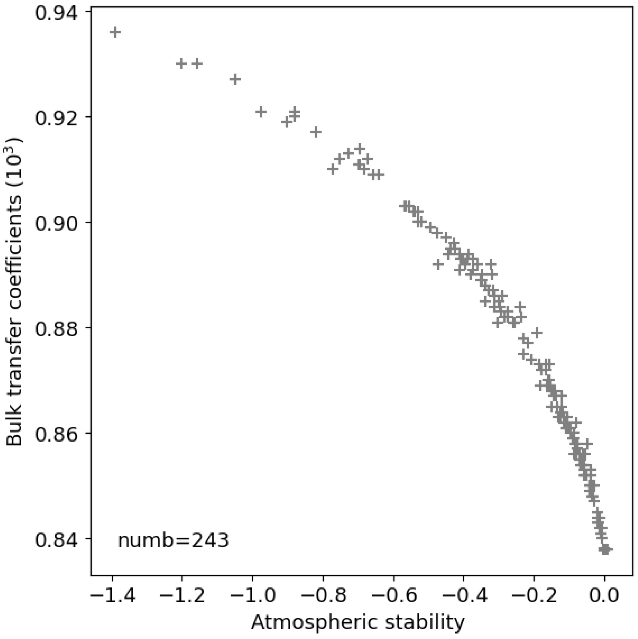
The bulk transfer coefficient Ch, was calculated indirectly using the bulk transfer method [47]. The Ch clearly varies in response to temporal changes in atmospheric stability (Figure 5). The Ch varied depending on atmospheric stability, as can be seen from Equation (6). The atmospheric stability was mostly unstable, probably because most dropsonde observations were made around 1:00 PM, when SST was higher than the air temperature. The Ch varied from 0.84 × 10⁻³ to 0.94 × 10⁻³, which was not significantly different from the values proposed in previous studies over the sea [5,7,50,51,52].
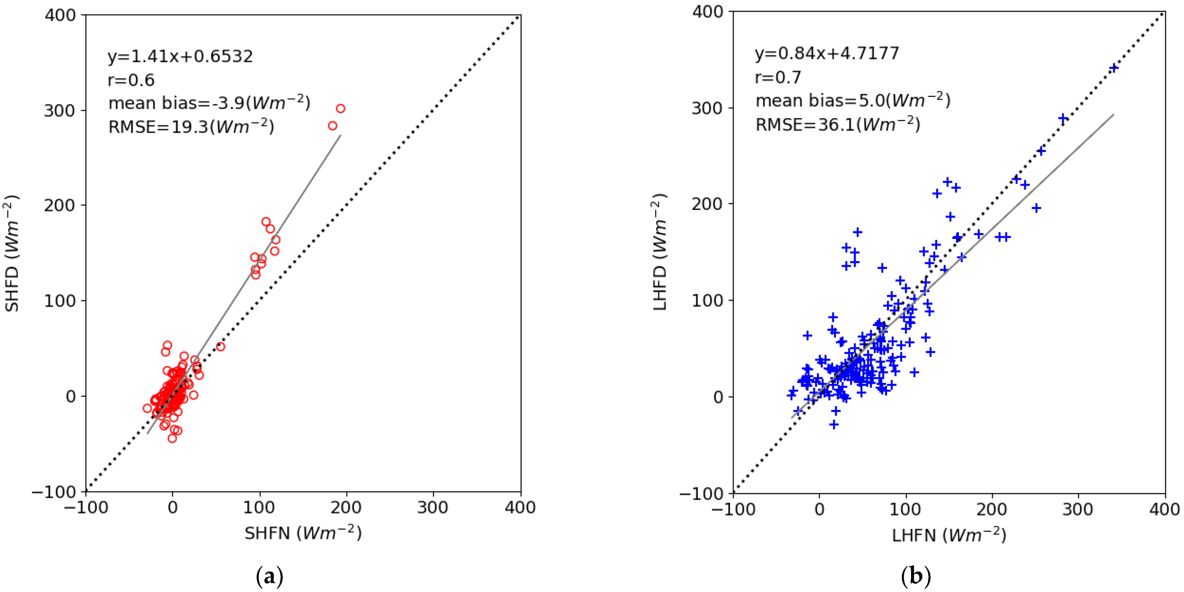
The dropsonde-based SHF (SHFD) and dropsonde-based LHF (LHFD) were estimated using Ch and compared with SHFN and LHFN, respectively. Figure 6 shows a linear relationship between the SHFD and the SHFN, with a correlation coefficient of 0.6, a mean bias of −3.9 W m−2, and a RMSE of 19.3 W m−2, which is less than approximately 10% of the maximum SHFN. In the presence of high sensible heat flux, the difference increased, and SHFD exceeded 100 W m−2. The comparison of the LHFD and LHFN shows good agreement, with a correlation coefficient of 0.7, a mean bias of 5.0 W m−2, and a RMSE of 36.1 W m−2, which is less than approximately 10% of the maximum LHFN. We confirmed that the bulk transfer method is useful for estimating SHFD and LHFD. Petersen and Renfrew [16] reported that model-based heat fluxes were over 100 W m−2 less than the aircraft-based direct flux measurements (i.e., eddy covariance method). Furthermore, they suggested that the lack of direct observations in extreme situations (i.e., in conditions of high wind speed, at high latitudes, and in a region where there are frequently large ocean-atmosphere temperature and humidity gradients) may result in an underestimation of the transfer coefficients in such situations, and thus an underestimation of model-based heat fluxes. They also suggested that flux parameterization schemes are based on large observational datasets, mostly ship-based observations, and that many of these observations are from the less direct inertial dissipation method. Bharti et al. [19] reported that reanalysis flux products perform poorly, with biases as high as 100 W m−2 over the Southern Ocean. The biases in model-based heat flux can be attributed to a higher bias in air temperature (10 m) and wind speed (10 m) at lower latitudes and in SST at higher latitudes. According to Bae et al. [53], the lack of ocean observation platforms contributes to uncertainty in calculating the heat transfer coefficient based on the heat flux parameterization. Given that the systematic limit, such as coarse spatial resolution and interpolation smoothing is the cause of model-based heat flux underestimation, SHFD and LHFD can be regarded as in situ observations obtained using the direct eddy covariance method [19].
Figure 7a shows the sensible heat flux depending on the difference (△ θ ) between the OISST-based virtual potential temperature θ 0 (K) and dropsonde-based virtual potential temperature θ 10 (K) based on 243 dropsonde profiles. The SHFD tended to increase when △ θ was increased and decrease when it was decreased. A negative SHFD indicates that heat is transferred to the sea from the atmosphere. In spring and summer, when △ θ is small, there is almost no heat exchange via SHFD, whereas the heat inflow from the ocean to the atmosphere significantly increases in late autumn and winter when the △ θ is relatively large, and the wind speed is high. In particular, the magnitudes of SHFD and LHFD in winter were nearly twice as large as those estimated in summer. Figure 7b shows a scatter plot of seasonal LHFD and the difference (ΔQ) between the dropsonde-based saturation mixing ratio Q 0 (g kg−1) closest to the sea level using OISST and the dropsonde-based mixing ratio Q 10 (g kg−1) at a reference height (approximately 10 m). In general, as ΔQ increases, so does the LHFD. The △Q remained low in the spring but increased from summer to autumn and winter when the atmosphere was dry. The amount of evaporation in the ocean due to the difference in humidity between the ocean and the atmosphere greatly affects the LHFD during the season when ΔQ is high. Unlike the SHFD, the wind speed difference (Figure 7c) contributed proportionally to the LHFD. Ritcher et al. [54] stated that they found no statistically significant trend, of the bulk transfer coefficient Ch with wind speeds up to roughly 20 m s−1. They also hypothesize that the influence spray is nonexistent in some way to yield unchanged flux coefficient. Fairall et al. [21] reported that spray droplet effects on the order of 10 W m−2 for the Humidity Exchange Over the Sea program-type conditions where direct evaporation is about 250 W m−2 and stated that bulk heat fluxes to be accurate within 5% for wind speeds of 0–10 m s−1 and 10% for wind speeds of between 10 and 20 m s−1. It was assumed that the dropsonde wind speed at the altitude of 10 m used in this study was less than 20 m s−1 and that the sea-spray effect could be ignored. From spring to autumn, the SHFD in all sea areas is less than 20 W m−2. In particular, a negative SHFD partially appears in the southern ES and WS during the summer. A negative SHFD indicates that heat flows from the atmosphere into the ocean. From autumn, the SHFD gradually increased from high latitudes, and it can be seen that the largest SHFD appeared in winter. Considering the characteristics of the LHFD shown in Figure 6 similar to the SHFD, it shows a low value in spring and summer but increases from autumn, showing the highest value of 160–360 W m−2 in winter. Sobel et al. [55] suggest that stronger (weaker) wind speeds over the off-equatorial regions increase (reduce) the LHFD and increase (decrease) SST. High (low) LHFD over the warm pool can be sustained because the incoming solar radiation is partially offset by ocean heat flux convergence (divergence) [55,56].
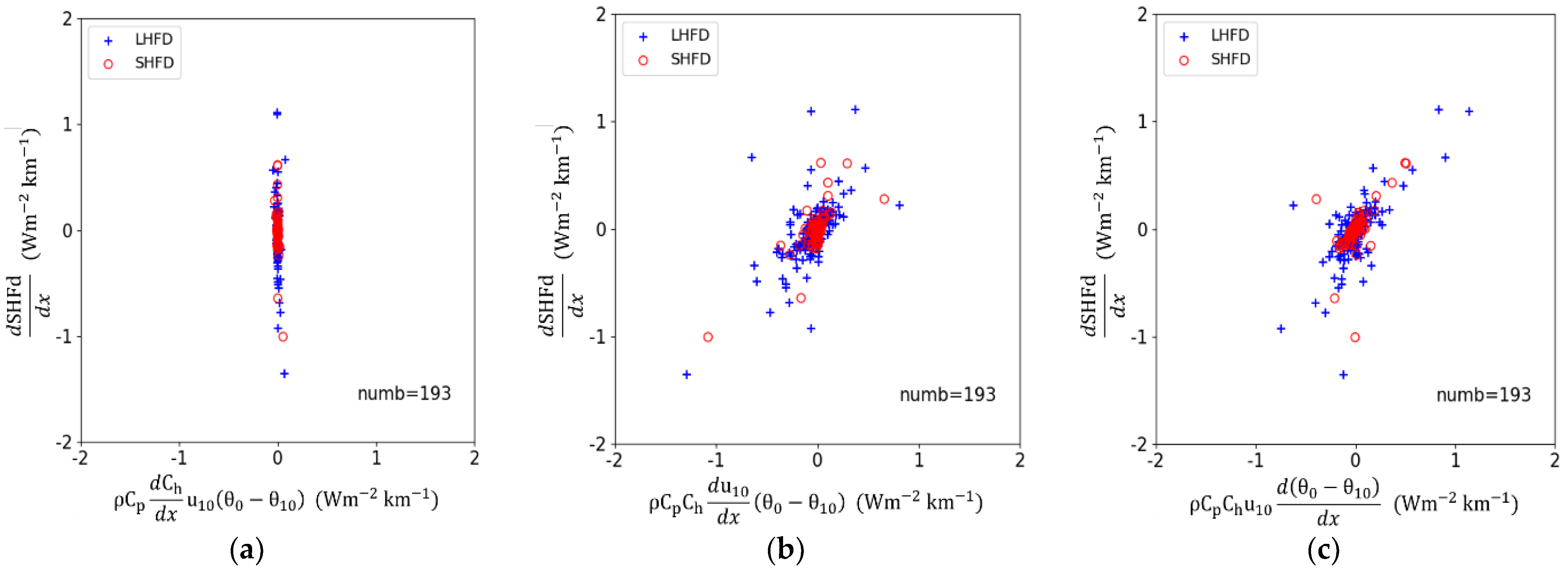
We also evaluated the contribution of spatial bulk parameters, variation of Ch, wind speed (dynamic term), △ θ = θ 0 θ 10 and △Q = Q 0 Q 10 (thermodynamic term) to the heat flux variation. These terms were derived from Equations (1) and (2) with respect to the horizontal distance (Figure 8). The spatial variation of SHFD and LHFD was investigated using 193 dropsonde observations (Table 1). Since the bulk transfer coefficients are a function of stability (see Figure 5), the first term on the right side indicates the variation in stability. This stability term is negligible in the heat flux along the flight axis (Figure 8a). Figure 8b shows the variation in heat fluxes based on the wind force. Heat fluxes increase as the wind speed increases. The heat flux, in particular, appears to decrease as the wind weakens. Figure 8c shows the variation of sensible heat flux based on the variation of △T and the variation of latent heat flux based on △Q. Notably, as the vertical difference of thermodynamic parameters increased, so did the variation of heat fluxes. Kwon et al. [48] reported that the dynamic and thermodynamic terms can operate in the same or opposite sense and that the heat fluxes during the low-pressure period were completely dependent on the thermodynamic characteristics of the incoming air mass during the low-pressure period. In this study, the thermodynamic term prevailed and resulted from the southward flight trajectories from the cold to warm zone. The increase in the thermodynamic term was associated with an increase in SST across the SST gradient. The air temperature increased in relatively quickly where the SST is higher and △ θ increases. When the air temperature increases, the saturated vapor pressure and △Q increase. SST horizontal gradients cause surface turbulent heat fluxes to have horizontal gradients [57].
dSHFD dx =   ρ C p { dC h dx [   u 10 ( θ 0 θ 10 ) ] + C h du 10 dx ( θ 0 θ 10 ) +   C h u 10 d dx ( θ 0 θ 10 ) }  
dLHFD dx =   ρ L v { dC q dx [   u 10 ( Q 0 Q 10 ) ] + C q du 10 dx ( Q 0 Q 10 ) +   C q u 10 d dx ( Q 0 Q 10 ) }

3.3. Marine Atmospheric Boundary Layer

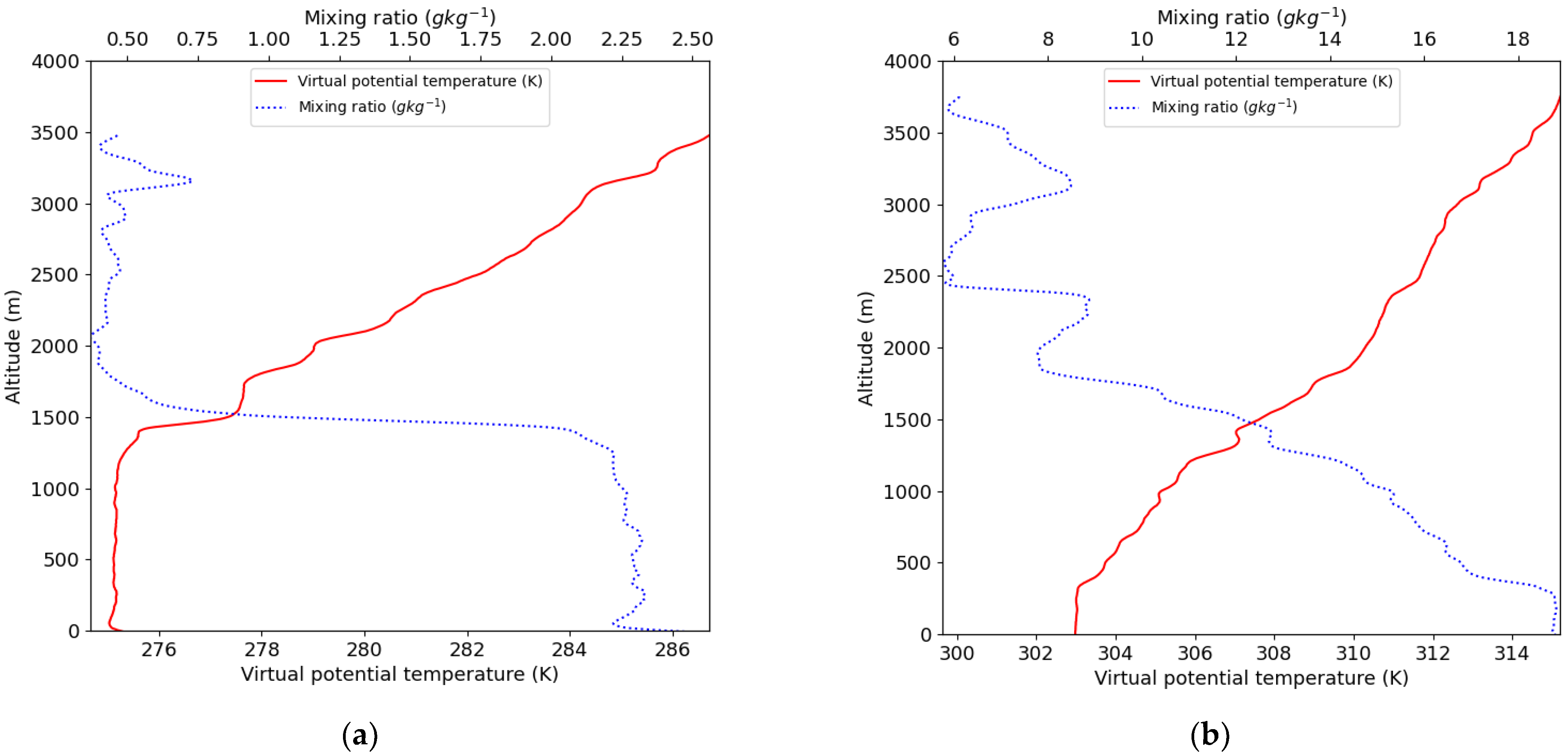
Figure 9 shows the dropsonde-based virtual potential temperature (red solid) and mixing ratio (blue dotted) profiles launched from the NARA at 13:51:41 KST in Case 1 and 14:16:59 KST in Case 2, respectively, and the dropsonde-induced MABL height was 1250 m and 250 m, respectively. The MABL in Case 1 was greater than that in Case 2 because both SHFD and LHFD were greater. The SHFD of Case 1 and Case 2 was 41.5 W m−2 and 0.3 W m−2, respectively, and the LHFD was 94.6 W m−2 and 28.9 W m−2, respectively. The SHFD and LHFD in Case 1 were higher than those in Case 2; △ θ and △Q during winter were larger than △ θ and △Q in summer. The dropsonde-based buoyancy flux (BFD) in Case 1 (42.2 W m−2) was also greater than that in Case 2 (0.5 W m−2). The △ θ in winter and summer was approximately 4.2 °C and 0.2 °C, respectively, and the △Q was approximately 4 g kg−1 and 3 g kg−1, respectively. The wind speeds at approximately 10 m were approximately 8.9 m s−1 and 3.1 m s−1 in winter and summer, respectively.

4. Discussion

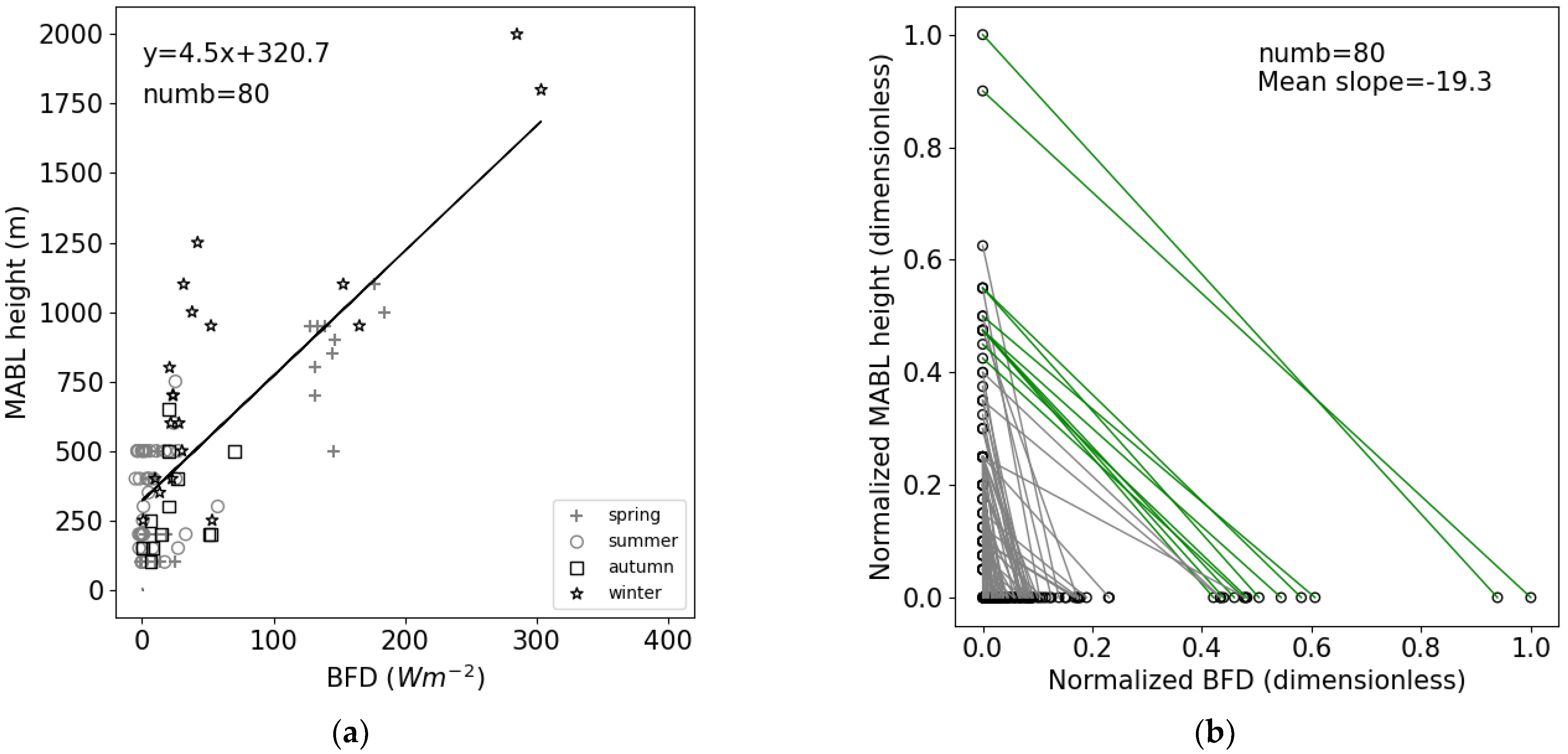
The BFD was estimated using SHFD and LHFD from Equation (3). The dependence of the MABL height on the BFD is illustrated in Figure 10a. As BFD increased, the MABL height also increased. The BFD ranged from 0 W m−2 to 300 W m−2 with the MABL height increasing up to 2 km. Because △ θ , △Q, and wind speed were higher in the ES than in the WS, MABL height and BFD were mainly higher in the ES in winter (Figure 10a). In summer, BFD reached 57.5 W m−2, with a mean MABL height of 358.3 m (Figure 10a). The lower the latitude in summer, the smaller the BFD, owing to the smaller ΔT. In autumn, the BFD ranged from 0.3–70.0 W m−2 with the mean BFD being 20.6 W m−2, and the mean MABL height being 300.0 m. Summer and autumn MABL heights were generally lower than spring MABL heights. In winter, the BFD values were 0.1–303.6 W m−2, the mean BFD was 65.1 W m−2, and the mean MABL height was 826.3 m. When the BFD increased, the MABL height also tended to increase. In particular, when △ θ , △Q, and wind speed were larger in the ES in winter, the MABL depth also increased owing to the transfer of much heat from the sea level to the atmosphere. In winter, the value of BFD, such as in spring, was higher in the ES than in the WS. The summer had the lowest mean BFD, while the winter had the highest. Especially during spring and summer, the BFD values were often negative, indicating heat transfer from the atmosphere to sea level. It was confirmed that most MABL heights were also high during the season when BFD was high. Kim et al. [58] reported that the buoyancy flux can be erroneously underestimated due to an underestimation of SST, especially in summer when the temperature difference between the atmosphere and the ocean is small.
The BFD is assumed to decrease with height and reach zero at the top of the MABL. The vertical profiles of the BFD normalized by the maximum BFD, according to the MABL height normalized by the maximum MABL height, using 80 vertical profiles that can determine the MABL height, are shown in Figure 10b. The slope is close to −1 at 120 W m−2 or more, which is 0.4 times the maximum value of BFD, and at 800 m or more, which is 0.4 times the maximum value of the MABL height. Therefore, it is possible to estimate the MABL height if the BFD is greater than 120 W m−2 (green lines). Specifically, if the bulk transfer method is used without directly measuring the turbulence, the MABL height can be determined using only the more easily measured mean quantities (sea surface temperature, air temperature, humidity, and wind speed). However, future studies should focus on the relationship between BFD and MABL height using more dropsonde observation cases. Although the comparison of the dropsonde and NARA atmospheric instrument (e.g., AIMMS-20) showed good agreement [22], it is not easy to obtain an accurate SST to determine heat fluxes based on the Monin-Obukhov similarity. This is a limitation of estimating dropsonde-based heat fluxes. Possible solutions could include using the gradient method [37] or the profile method [58] which does not require SST, and using dropsonde with infrared sensor to estimate SST [7,47].

5. Conclusions

The seas serve as a large source/sink and reservoir of heat energy, transferring it from the sea to the atmosphere and vice versa. For the first time in Korea, the dropsonde-based sensible heat flux (SHFD) and latent heat flux (LHFD) were estimated using dropsonde observation data from the NARA in this study. The SHFD and LHFD over the seas were estimated using the bulk transfer method, and they were compared and analyzed with model-based sensible heat flux (SHFN) and latent heat flux (LHFN). The SHFD and LHFD were found to be overestimated when compared with SHFN and LHFN. When the sensible heat flux is high, the difference grows, and SHFD exceeds up to 100 W m−2. We can consider SHFD and LHFD as in situ observations obtained by the direct eddy covariance method by considering that the cause of the underestimation of model-based heat fluxes is the systematic limit, such as coarse spatial resolution and smoothing by interpolation. The SHFD showed a tendency to increase when △ θ increased and to decrease when it decreased. The LHFD and △Q showed the same tendency to increase/decrease and were relatively more sensitive to wind speed than SHFD. We also evaluated the contribution of the spatial bulk parameters, variation in stability, dynamic term, and thermodynamic term to the heat flux variation. The increase in the thermodynamic term is linked to an increase in SST across the SST gradient. The air temperature increases relatively quickly when the SST is higher and △ θ increases. When the air temperature increases, the saturated vapor pressure and △Q increase. In addition, a method for estimating MABL height using dropsonde-based buoyancy flux data was proposed. The slope was close to −1 at 120 W m−2 or more, which was 0.4 times the maximum value of BFD, and at 800 m or more, which was 0.4 times the maximum value of the MABL height. This study proposes a relationship between the heat flux estimates derived from dropsondes and the MABL height observed by dropsondes as guides for estimating MABL height using only more easily measured mean quantities. Since dropsondes data have been accumulated, it will be possible to determine the threshold of buoyancy flux to estimate the MABL height in future studies. This study could contribute to enhancing the scientific understanding of heat fluxes and MABL over the sea around the Korean.
This study also calls for further analyses of the uncertainty in the mean measurements such as dropsonde and SST, heat transfer coefficients, and heat fluxes. We plan to investigate the further analyses of the sensitivity experiments by using eddy covariance heat fluxes and SST observation data from the Ieodo Ocean Research Station (32.12°N, 125.18°E) and also perform a seasonal analysis.

Author Contributions

Conceptualization, M.-S.K. and B.H.K.; methodology, M.-S.K. and B.H.K.; formal analysis, M.-S.K. and B.H.K.; validation, M.-S.K.; investigation, M.-S.K.; visualization, M.-S.K.; writing—original draft preparation, M.-S.K.; writing—review and editing, M.-S.K. and B.H.K.; supervision, T.-Y.G. and B.H.K.; project administration, S.-P.J. and T.-Y.G.; funding acquisition, S.-P.J. and T.-Y.G. All authors have read and agreed to the published version of the manuscript.

Funding

This work was funded by the Korea Meteorological Administration Research and Development Program ‘Developing Application Technology for Atmospheric Research Aircraft’ under Grant (KMA2018-00222).

Data Availability Statement

The OISST v2.1 data are available at NOAA/NCEI (https://www.ncei.noaa.gov/products/optimum-interpolation-sst, accessed on 18 December 2022). The SeaFlux-CDR data are provided at NOAA National Center for Environmental Information (doi:10.7289/V59K4885).

Acknowledgments

We would like to thank the editors and the anonymous reviewers for their comments, which helped in the substantial improvement of this manuscript. We thank the Korea Meteorological Administration, National Oceanic and Atmospheric Administration and National Center for Environmental Information for the dataset.

Conflicts of Interest

The authors declare no conflict of interest.

References

  1. Khim, J.S.; Lee, C.; Song, S.J.; Bae, H.; Noh, J.; Lee, J.; Kim, H.G.; Choi, J.W.; Seong Khim, J.; Lee, C.; et al. Marine biodiversity in Korea: A review of macrozoobenthic assemblages, their distributions, and long-term community changes from human impacts. In Oceanography and Marine Biology: An Annual Review; CRC Press: Boca Raton, FL, USA, 2021. [Google Scholar]
  2. Farach-Espinoza, E.B.; López-Martínez, J.; García-Morales, R.; Otilio Nevárez-Martínez, M.; Lluch-Cota, D.B.; Ortega-García, S. Temporal variability of oceanic mesoscale events in the Gulf of California. Remote Sens. 2021, 13, 1774. [Google Scholar] [CrossRef]
  3. Park, J.E.; Park, K.A.; Kang, C.K.; Park, Y.J. Short-Term Response of Chlorophyll-a Concentration to Change in Sea Surface Wind Field over Mesoscale Eddy. Estuaries Coasts 2020, 43, 646–660. [Google Scholar] [CrossRef]
  4. Curry, J.A.; Bentamy, A.; Bourassa, M.A.; Bourras, D.; Bradley, E.F.; Brunke, M.; Castro, S.; Chou, S.H.; Clayson, C.A.; Emery, W.J.; et al. SEAFLUX. Bull. Am. Meteorol. Soc. 2004, 85, 409–424. [Google Scholar] [CrossRef] [Green Version]
  5. Praveen Kumar, B.; Cronin, M.F.; Joseph, S.; Ravichandran, M.; Sureshkumar, N. Latent Heat Flux Sensitivity to Sea Surface Temperature: Regional Perspectives. J. Clim. 2017, 30, 129–143. [Google Scholar] [CrossRef]
  6. Ming, J.; Zhang, J.A. Effects of surface flux parameterization on the numerically simulated intensity and structure of Typhoon Morakot (2009). Adv. Atmos. Sci. 2015, 33, 58–72. [Google Scholar] [CrossRef]
  7. Zhang, J.A.; Cione, J.J.; Kalina, E.A.; Uhlhorn, E.W.; Hock, T.; Smith, J.A. Observations of Infrared Sea Surface Temperature and Air–Sea Interaction in Hurricane Edouard (2014) Using GPS Dropsondes. J. Atmos. Ocean. Technol. 2017, 34, 1333–1349. [Google Scholar] [CrossRef]
  8. Wu, L.; Wang, B.; Braun, S.A. Impacts of Air–Sea Interaction on Tropical Cyclone Track and Intensity. Mon. Weather Rev. 2005, 133, 3299–3314. [Google Scholar] [CrossRef] [Green Version]
  9. Yun, K.S.; Chan, J.C.L.; Ha, K.J. Effects of SST magnitude and gradient on typhoon tracks around East Asia: Acase study for Typhoon Maemi (2003). Atmos. Res. 2012, 109–110, 36–51. [Google Scholar] [CrossRef]
  10. Song, Q.; Cornillon, P.; Hara, T. Surface wind response to oceanic fronts. J. Geophys. Res. Ocean. 2006, 111, 12006. [Google Scholar] [CrossRef]
  11. Liu, W.T.; Xie, X.; Niiler, P.P. Ocean–Atmosphere Interaction over Agulhas Extension Meanders. J. Clim. 2007, 20, 5784–5797. [Google Scholar] [CrossRef]
  12. Businger, J.A. Evaluation of the Accuracy with Which Dry Deposition Can Be Measured with Current Micrometeorological Techniques. J. Appl. Meteorol. Climatol. 1986, 25, 1100–1124. [Google Scholar] [CrossRef]
  13. Cronin, M.F.; Gentemann, C.L.; Edson, J.B.; Ueki, I.; Bourassa, M.; Brown, S.; Clayson, C.A.; Fairall, C.; T. Farrar, J.; Gille, S.T.; et al. Air-sea fluxes with a focus on heat and momentum. Front. Mar. Sci. 2019, 6, 430. [Google Scholar] [CrossRef] [Green Version]
  14. Kubota, M.; Iwasaka, N.; Kizu, S.; Konda, M.; Kutsuwada, K. Japanese Ocean Flux Data Sets with Use of Remote Sensing Observations (J-OFURO). J. Oceanogr. 2002, 58, 213–225. [Google Scholar] [CrossRef]
  15. Shie, C.L.; Chiu, L.S.; Adler, R.; Nelkin, E.; Lin, I.I.; Xie, P.; Wang, F.C.; Chokngamwong, R.; Olson, W.; Chu, D.A. A note on reviving the Goddard Satellite-based Surface Turbulent Fluxes (GSSTF) dataset. Adv. Atmos. Sci. 2009, 26, 1071–1080. [Google Scholar] [CrossRef]
  16. Andersson, A.; Fennig, K.; Klepp, C.; Bakan, S.; Graßl, H.; Schulz, J. The Hamburg ocean atmosphere parameters and fluxes from satellite data-HOAPS-3. Earth Syst. Sci. Data 2010, 2, 215–234. [Google Scholar] [CrossRef] [Green Version]
  17. Bentamy, A.; Desbiolles, F.; Grodsky, S.A.; Katsaros, K.; Mestas-Nuñez, A.M.; Blanke, B.; Desbiolles, F. Improvement in air–sea flux estimates derived from satellite observations. Int. J. Remote Sens. 2013, 34, 5243–5261. [Google Scholar] [CrossRef] [Green Version]
  18. Renfrew, I.A.; Petersen, G.N.; Sproson, D.A.J.; Moore, G.W.K.; Adiwidjaja, H.; Zhang, S.; North, R. A comparison of aircraft-based surface-layer observations over Denmark Strait and the Irminger Sea with meteorological analyses and QuikSCAT winds. Q. J. R. Meteorol. Soc. 2009, 135, 2046–2066. [Google Scholar] [CrossRef] [Green Version]
  19. Bharti, V.; Schulz, E.; Fairall, C.W.; Blomquist, B.W.; Huang, Y.I.; Protat, A.; Siems, S.T.; Manton, M.J. Assessing Surface Heat Flux Products with In Situ Observations over the Australian Sector of the Southern Ocean. J. Atmos. Ocean. Technol. 2019, 36, 1849–1861. [Google Scholar] [CrossRef] [Green Version]
  20. Petersen, G.N.; Renfrew, I.A. Aircraft-based observations of air–sea fluxes over Denmark Strait and the Irminger Sea during high wind speed conditions. Q. J. R. Meteorol. Soc. 2009, 135, 2030–2045. [Google Scholar] [CrossRef]
  21. Fairall, C.W.; Bradley, E.F.; Hare, J.E.; Grachev, A.A.; Edson, J.B. Bulk parameterization of air-sea fluxes: Updates and verification for the COARE algorithm. J. Clim. 2003, 16, 571–591. [Google Scholar] [CrossRef]
  22. Kim, J.-H.; Goo, T.-Y.; Jung, S.-P.; Kim, M.-S.; Lee, K.; Kang, M.; Lee, C.; Yang, J.; Hong, S.; Ko, H.; et al. Overview of the KMA/NIMS Atmospheric Research Aircraft (NARA) and its data archive: Annual airborne observations over the Korean peninsula. Geosci. Data J. 2022, in press. [Google Scholar] [CrossRef]
  23. Li, S.; Kim, Y.; Kim, J.; Takele, S.; Goo, T.Y.; Labzovskii, L.D.; Byun, Y.H. In Situ Aircraft Measurements of CO2 and CH4: Mapping Spatio-Temporal Variations over Western Korea in High-Resolutions. Remote Sens. 2020, 12, 3093. [Google Scholar] [CrossRef]
  24. Yeh, S.W.; Kim, C.H. Recent warming in the Yellow/East China Sea during winter and the associated atmospheric circulation. Cont. Shelf Res. 2010, 30, 1428–1434. [Google Scholar] [CrossRef]
  25. Kim, K.; Kim, K.R.; Kim, Y.G.; Cho, Y.K.; Kang, D.J.; Takematsu, M.; Volkov, Y. Water masses and decadal variability in the East Sea (Sea of Japan). Prog. Oceanogr. 2004, 61, 157–174. [Google Scholar] [CrossRef]
  26. George, G.; Stevens, B.; Bony, S.; Klingebiel, M.; Vogel, R. Observed Impact of Mesoscale Vertical Motion on Cloudiness. J. Atmos. Sci. 2021, 78, 2413–2427. [Google Scholar]
  27. Reynolds, R.W.; Smith, T.M.; Liu, C.; Chelton, D.B.; Casey, K.S.; Schlax, M.G. Daily High-Resolution-Blended Analyses for Sea Surface Temperature. J. Clim. 2007, 20, 5473–5496. [Google Scholar] [CrossRef]
  28. Banzon, V.; Smith, T.M.; Mike Chin, T.; Liu, C.; Hankins, W. A long-term record of blended satellite and in situ sea-surface temperature for climate monitoring, modeling and environmental studies. Earth Syst. Sci. Data 2016, 8, 165–176. [Google Scholar] [CrossRef] [Green Version]
  29. Jang, J.C.; Park, K.A. High-Resolution Sea Surface Temperature Retrieval from Landsat 8 OLI/TIRS Data at Coastal Regions. Remote Sens. 2019, 11, 2687. [Google Scholar] [CrossRef] [Green Version]
  30. Stolzenberger, S.; Rietbroek, R.; Wekerle, C.; Uebbing, B.; Kusche, J. Simulated signatures of Greenland melting in the North Atlantic: A model comparison with Argo floats, satellite observations, and ocean reanalysis. J. Geophys. Res. Ocean. 2022, 127, e2022JC018528. [Google Scholar] [CrossRef]
  31. Huang, B.; Liu, C.; Freeman, E.; Graham, G.; Smith, T.; Zhang, H.M. Assessment and Intercomparison of NOAA Daily Optimum Interpolation Sea Surface Temperature (DOISST) Version 2.1. J. Clim. 2021, 34, 7421–7441. [Google Scholar] [CrossRef]
  32. Huang, B.; Liu, C.; Banzon, V.; Freeman, E.; Graham, G.; Hankins, B.; Smith, T.; Zhang, H.M. Improvements of the Daily Optimum Interpolation Sea Surface Temperature (DOISST) Version 2.1. J. Clim. 2021, 34, 2923–2939. [Google Scholar] [CrossRef]
  33. Lee, E.Y.; Park, K.A. Validation of Satellite Sea Surface Temperatures and Long-Term Trends in Korean Coastal Regions over Past Decades (1982–2018). Remote Sens. 2020, 12, 3742. [Google Scholar] [CrossRef]
  34. Yang, W.; John, V.O.; Zhao, X.; Lu, H.; Knapp, K.R. Satellite climate data records: Development, applications, and societal benefits. Remote Sens. 2016, 8, 331. [Google Scholar] [CrossRef] [Green Version]
  35. Rodell, M.; Beaudoing, H.K.; L’Ecuyer, T.S.; Olson, W.S.; Famiglietti, J.S.; Houser, P.R.; Adler, R.; Bosilovich, M.G.; Clayson, C.A.; Chambers, D.; et al. The Observed State of the Water Cycle in the Early Twenty-First Century. J. Clim. 2015, 28, 8289–8318. [Google Scholar] [CrossRef] [Green Version]
  36. Cuijpers, J.W.M.; Bechtold, P. A simple parameterization of cloud water related variables for use in boundary layer models. J. Atmos. Sci. 1995, 52, 2486–2490. [Google Scholar] [CrossRef]
  37. Businger, J.A.; Wyngaard, J.C.; Izumi, Y.; Bradley, E.F.; Businger, J.A.; Wyngaard, J.C.; Izumi, Y.; Bradley, E.F. Flux-Profile Relationships in the Atmospheric Surface Layer. J. Atmos. Sci. 1971, 28, 181–189. [Google Scholar] [CrossRef]
  38. Abbasi, A.; Annor, F.O.; van de Giesen, N. Effects of atmospheric stability conditions on heat fluxes from small water surfaces in (semi-)arid regions. Hydrol. Sci. J. 2017, 62, 1422–1439. [Google Scholar] [CrossRef] [Green Version]
  39. Arya, S.P. Introduction to Micrometeorology; Academic Press: Cambridge, MA, USA, 1988; ISBN 9788578110796. [Google Scholar]
  40. Deardorff, J.W. Parameterization of the Planetary Boundary layer for Use in General Circulation Models 1. Mon. Weather Rev. 1972, 100, 93–106. [Google Scholar] [CrossRef]
  41. Katz, J.; Zhu, P. Evaluation of surface layer flux parameterizations using in-situ observations. Atmos. Res. 2017, 194, 150–163. [Google Scholar] [CrossRef]
  42. Monin, A.S.; Obukhov, A.M. Basic laws of turbulent mixing in the surface layer of the atmosphere. Tr. Akad. Nauk SSSR Geophiz. Inst. 1954, 151, e187. [Google Scholar]
  43. Geernaert, G.L.; Larsen, S.E.; Hansen, F. Measurements of the wind stress, heat flux, and turbulence intensity during storm conditions over the North Sea. J. Geophys. Res. Ocean. 1987, 92, 13127–13139. [Google Scholar] [CrossRef]
  44. Hussein, M.M.A. Impact of atmospheric stability conditions on heat fluxes from Alexandria Eastern Harbor, Egypt. Egypt. J. Aquat. Res. 2019, 45, 313–319. [Google Scholar] [CrossRef]
  45. Verburg, P.; Antenucci, J.P. Persistent unstable atmospheric boundary layer enhances sensible and latent heat loss in a tropical great lake: Lake Tanganyika. J. Geophys. Res. Atmos. 2010, 115, 11109. [Google Scholar] [CrossRef]
  46. Launiainen, J.; Vihma, T. Derivation of turbulent surface fluxes—An iterative flux-profile method allowing arbitrary observing heights. Environ. Softw. 1990, 5, 113–124. [Google Scholar] [CrossRef]
  47. Kim, M.-S.; Kwon, B.H. Estimation of sensible heat flux and atmospheric boundary layer height using an unmanned aerial vehicle. Atmosphere 2019, 10, 363. [Google Scholar] [CrossRef] [Green Version]
  48. Kwon, B.H.; Bénech, B.; Lambert, D.; Durand, P.; Druilhet, A.; Giordani, H.; Planton, S. Structure of the marine atmospheric boundary layer over an oceanic thermal front: SEMAPHORE experiment. J. Geophys. Res. Ocean. 1998, 103, 25159–25180. [Google Scholar] [CrossRef]
  49. Foussard, A.; Lapeyre, G.; Plougonven, R. Response of Surface Wind Divergence to Mesoscale SST Anomalies under Different Wind Conditions. J. Atmos. Sci. 2019, 76, 2065–2082. [Google Scholar] [CrossRef]
  50. Zhang, J.A.; Black, P.G.; French, J.R.; Drennan, W.M. First direct measurements of enthalpy flux in the hurricane boundary layer: The CBLAST results. Geophys. Res. Lett. 2008, 35, L14813. [Google Scholar] [CrossRef] [Green Version]
  51. Haus, B.K.; Jeong, D.; Donelan, M.A.; Zhang, J.A.; Savelyev, I. Relative rates of sea-air heat transfer and frictional drag in very high winds. Geophys. Res. Lett. 2010, 37. [Google Scholar] [CrossRef]
  52. Bell, M.M.; Montgomery, M.T.; Emanuel, K.A. Air–Sea Enthalpy and Momentum Exchange at Major Hurricane Wind Speeds Observed during CBLAST. J. Atmos. Sci. 2012, 69, 3197–3222. [Google Scholar] [CrossRef]
  53. Bae, H.J.; Yang, S.; Jeong, T.B.; Yang, A.R.; Cha, D.H.; Lee, G.; Lee, H.Y.; Byun, D.S.; Kim, B.M. An Estimation of Ocean Surface Heat Fluxes during the Passage of Typhoon at the Ieodo Ocean Research Station: Typhoon Lingling Case Study 2019. Asia-Pac. J. Atmos. Sci. 2022, 58, 305–314. [Google Scholar] [CrossRef]
  54. Richter, D.H.; Bohac, R.; Stern, D.P. An assessment of the flux profile method for determining air–sea momentum and enthalpy fluxes from dropsonde data in tropical cyclones. J. Atmos. Sci. 2016, 73, 2665–2682. [Google Scholar] [CrossRef]
  55. Sobel, A.H. On the Coexistence of an Evaporation Minimum and Precipitation Maximum in the Warm Pool. J. Clim. 2003, 16, 1003–1009. [Google Scholar] [CrossRef]
  56. DiNezio, P.N.; Clement, A.C.; Vecchi, G.A.; Soden, B.J.; Kirtman, B.P.; Lee, S.K. Climate Response of the Equatorial Pacific to Global Warming. J. Clim. 2009, 22, 4873–4892. [Google Scholar] [CrossRef]
  57. Kim, M.S.; Kwon, B.H.; Goo, T.Y. Comparisons between Mean and Turbulent Parameters of Aircraft-Based and Ship-Based Measurements in the Marine Atmospheric Boundary Layer. Atmosphere 2021, 12, 1088. [Google Scholar] [CrossRef]
  58. Nieuwstadt, F. The computation of the friction velocity u * and the temperature scale T * from temperature and wind velocity profiles by least-square methods. Boundary-Layer Meteorol. 1978, 14, 235–246. [Google Scholar] [CrossRef]
Figure 1. Location of dropsondes release zones (gray circles) in the WS, ES, and SS of the Korea and buoy positions (black triangles).
Remotesensing 15 00025 g001
Figure 2. Comparison of OISST with the SST from buoys operating in the WS, ES, and SS of Korea.
Remotesensing 15 00025 g002
Figure 3. SST field and aircraft trajectories on (a) 3 February 2021, and (b) 2 August 2021. Each black triangle represents the point at which the dropsonde was launched from the NARA at an altitude of approximately 4 km in the WS. The solid white line represents the flight path of the aircraft.
Remotesensing 15 00025 g003
Figure 4. Variation in SST (red circle) and air temperature (blue square) along the flight path. The x-axis of (a) and (b) represents the distance from the initial launch point A of the dropsonde to the final point B over the West Sea. (a) 3 February 2021; (b) 2 August 2021; (c) the gradient of SST and air temperature.
Remotesensing 15 00025 g004
Figure 5. Bulk transfer coefficient Ch as a function of atmospheric stability.
Remotesensing 15 00025 g005
Figure 6. Comparison of dropsonde-based SHF (SHFD) and dropsonde-based LHF (LHFD) with model-based sensible heat flux (SHFN) and model-based latent heat flux (LHFN), respectively. (a) sensible heat flux (b) latent heat flux.
Remotesensing 15 00025 g006
Figure 7. Scatter plots of (a) sensible heat flux (SHFD) and ΔT, (b) latent heat flux (LHFD) and ΔQ, and (c) heat fluxes (SHFD and LHFD) and wind speed. (a) sensible heat flux; (b) latent heat flux; (c) wind effect.
Remotesensing 15 00025 g007
Figure 8. Contribution of spatial variation of bulk transfer coefficient Ch (stability term), wind speed (dynamic term), △ θ = θ 0 θ 10 and △Q = Q 0 Q 10 (thermodynamic term) to the heat fluxes variation. (a) stability term; (b) dynamic term; (c) thermodynamic term.
Remotesensing 15 00025 g008
Figure 9. Dropsonde-based virtual potential temperature and mixing ratio profiles. The blue dotted and red solid lines represent mixing ratio and virtual potential temperature profiles. (a) 3 February 2021; (b) 2 August 2021.
Remotesensing 15 00025 g009
Figure 10. Development of MABL heights depending on the (a) BFD, and (b) the relationship between the normalized MABL height and the normalized BFD.
Remotesensing 15 00025 g010
Table 1. List of dropsondes launched in 2021.
Date Time
(KST)
SiteAvailable
Profile
DateTime
(LST)
SiteAvailable ProfileDateTime
(LST)
SiteAvailable
Profile
21 January 15WS127 May 13–14WS52 August13–14WS4
22 January13–14ES48 June 13–14WS67 August13–14WS3
27 January13–14WS210 June 13–14WS69 August 13–14WS3
29 January 13ES218 June14–15SS712 August13–14WS6
1 February14WS222 June 13–14WS620 August 09–10WS6
3 February14WS423 June13–14WS621 August 08–09WS4
4 February13ES225 June13–14WS623 August 08–09WS6
25 February13–14WS428 June 13–14WS624 August 08–09WS5
2 March14ES429 June 13–14WS631 August 08–10WS6
6 March13–14ES61 July 13–15SS81 September08–09WS6
9 March13WS23 July13–14SS 46 September09–10WS6
17 March13–14WS45 July 13–15SS712 September09–10SS10
26 March13–14WS47 July13–14SS813 September09–10WS6
30 March13–14WS39 July13–14SS814 September09–10WS6
23 April 13–14WS627 July 13–14WS618 November15WS2
11 May 13–14WS529 July13–14WS5
20 May 13–14WS630 July13–14WS3
Disclaimer/Publisher’s Note: The statements, opinions and data contained in all publications are solely those of the individual author(s) and contributor(s) and not of MDPI and/or the editor(s). MDPI and/or the editor(s) disclaim responsibility for any injury to people or property resulting from any ideas, methods, instructions or products referred to in the content.