Satellite Imaging Techniques for Ground Movement Monitoring of a Deep Pipeline Trench Backfilled with Recycled Materials

Abstract

The damage to pipeline infrastructures caused by reactive soils has been a critical challenge for asset owners. Sustainable backfilling materials have recently gained interest to stabilize highly reactive zones as a pre-emptive approach towards sustainability. In this study, two adjacent sections of a sewer pipeline trench in Melbourne, Australia were backfilled with two blends of 100% recycled aggregates. The sites were monitored for ground deformations during October 2020–February 2022 (17 months) using surveying techniques. Interferometric synthetic aperture radar (InSAR) techniques and algorithms were also employed to estimate the ground movements of the sites and surrounding regions. The cross-validation of deformation results achieved from both techniques enabled an in-depth analysis of the effectiveness of the recycled aggregates to address reactive soil issues in urban developments. Observational deformation data and their spatiotemporal variation in the field were satisfactorily captured by the InSAR techniques: differential InSAR (DInSAR), persistent scatterer interferometry (PSI), and small baseline subset (SBAS). The SBAS estimations were found to be the closest to field measurements, primarily due to the analysis of zones without well-defined geometries. This study’s contribution to existing knowledge defines the spatiotemporal influence of sustainable backfill in areas with reactive soil through field data and satellite imaging. The relationship between InSAR techniques and actual field behavior of sustainable backfill can be a baseline for the growing construction that may be challenging to perform field monitoring due to resource constraints.

1. Introduction

The shrink–swell ground movement of reactive soils, in response to their moisture content variations, threatens the structural integrity of lightweight infrastructures leading to detrimental social and economic impacts on the community [1,2]. A common challenge presented by reactive soil movements involves the damage to urban and suburban sewer pipeline infrastructures [3]. The significant volume change of reactive soils due to the changes in moisture content causes severe damage to sewer pipe networks [3]. The 2008 report by [4] estimated the total annual cost for maintenance, repair, and replacement of buried pipes in Australia to be more than 7.5 billion over five years, which is almost 10% of the cost required to replace the entire Australian pipe networks. Furthermore, there is an increased risk of reactive soil damage to sewer pipe infrastructures in Australia since these reactive clays vastly cover developed and growth areas, with approximately 20% of the land area covering the entirety of Australia [5,6].

Sewer pipe infrastructures backfilled with available reactive soils on site are more susceptible to damage caused by the seasonal shrinking and swelling [7,8,9]. Rajeev and Kodikara [3] observed that the pipelines buried in areas having high-plasticity clays experienced a high frequency of damage, which portrays the role of significant volume change in reactive soils on pipe damage. Moreover, most of the damage that occurred in the buried pipes was when soil moisture abruptly increased after the dry season. The damage was more severe on small-diameter sewer pipes in narrow trenches installed deeper than 1.5 m [3]. This is mainly because of safety limitations and a lack of acceptable quality control in the field.

Various blends of recycled materials have been identified as a viable alternative to problematic reactive soil backfill due to their low moisture sensitivity and compaction requirement contributing to sustainable construction [10,11]. Recycled plastic, glass, and tire have been investigated as replacement materials for various applications, with most studies only partially replacing conventional materials [12,13,14]. In contrast, [15] utilized blends that comprised 100% recycled material as trench backfill materials. Their study proposed two sustainable blends with optimum performances for backfilling deep sewer trenches in non-trafficable areas through extensive environmental and geotechnical testing programs [15]. Ref. [16] investigated the field performance of the proposed blends by the construction of two full-scale trial sites in two adjacent areas in the west of Melbourne, Australia. Surveying techniques were used to measure the ground deformation in the sites using surveying techniques at a limited number of locations where settlement plates were installed. However, the spatiotemporal impact of the sustainable backfill (SB) on the two locations has not been thoroughly assessed.

Field monitoring of spatiotemporal ground movements is labor-intensive, time-consuming, and typically of low resolution. On the other hand, recent advancements in active remote sensing technology such as synthetic aperture radar (SAR), complemented with open-access software and improved computer capabilities, have enabled ground movement estimation in high resolution. SAR uses the phase difference between two or more complex satellite image acquisitions of the same area taken from almost similar satellite positions can be used to form interferometric SAR (InSAR). This technique measures the spatiotemporal changes in the ground surface [17].

Three main InSAR techniques have been used to obtain ground surface displacements in the literature. First, the differential InSAR (DInSAR) estimates the ground surface displacements that occurred between two acquisition dates considered as the reference and the secondary images [18]. Through the years, the methodology has improved and developed more advanced time-series techniques considering multiple satellite images collected within a specific period [19,20,21]. The remaining two techniques are persistent scatterer interferometry (PSI) and small baseline subset (SBAS). These time-series InSAR techniques alleviate the issues in the DInSAR method such as limitations in differentiating between the effect of displacement and the atmospheric signature [19]. The application of PSI and SBAS can exploit the phase history over a long period that can identify meaningful spatiotemporal trends. DInSAR, PSI, and SBAS have been applied to earthquakes [22], ground subsidence and heaving [23], landslides [24], mining [25], and volcanic activities [26].

This study investigates the feasibility of using InSAR analyses to estimate the spatiotemporal ground movements of a relatively smaller site where an SB was used to backfill a sewer trench detailed in [16]. The availability of field ground movement measurements for verification prompted the authors of the current study to select this site for InSAR analyses. Innovative applications of InSAR techniques (i.e., DInSAR, PSI, and SBAS) can enable a deeper understanding of the behavior and the impact of SB on the surrounding area. The outcomes of this study provide novel and robust analysis to evaluate the global applicability of blends of recycled aggregates as alternatives for conventional backfilling construction materials in highly reactive sites. Overall, the paired satellite imaging and field data collection presented in this study facilitate an efficient spatiotemporal evaluation of the effectiveness of novel applications of recycled materials contributing to a more resilient and sustainable geotechnical infrastructure.

2. Materials and Methods

Spatiotemporal field measurements of ground movements in the vicinity of sewer pipe trench sections in the west of Melbourne backfilled using blends of recycled materials were used in this study as the benchmarks for evaluating the reliability of InSAR estimations. The authors in [15,16] detail the blends used and the construction procedures. Below is a summary of the construction and field monitoring works followed by the InSAR analyzing procedure.

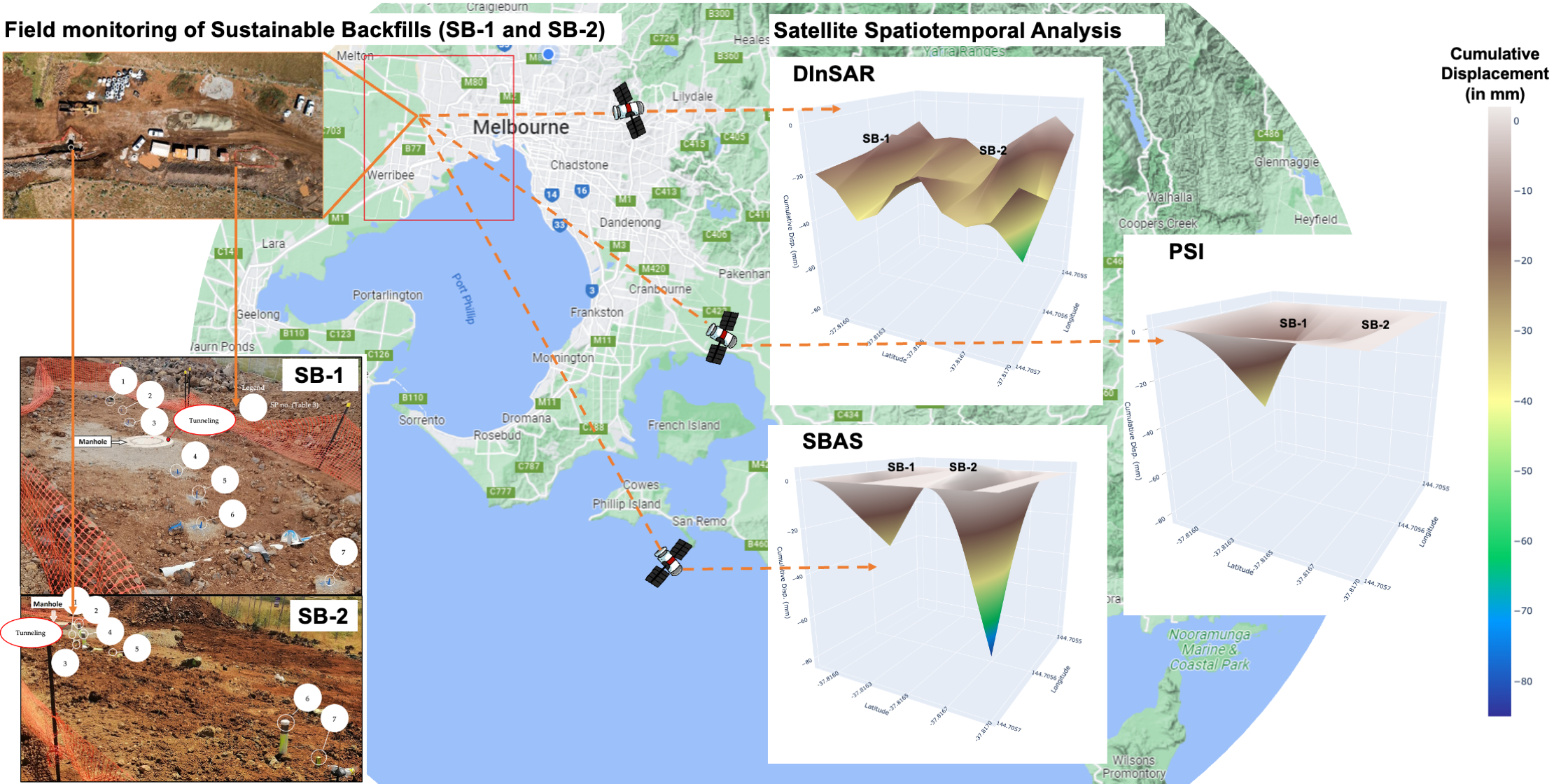
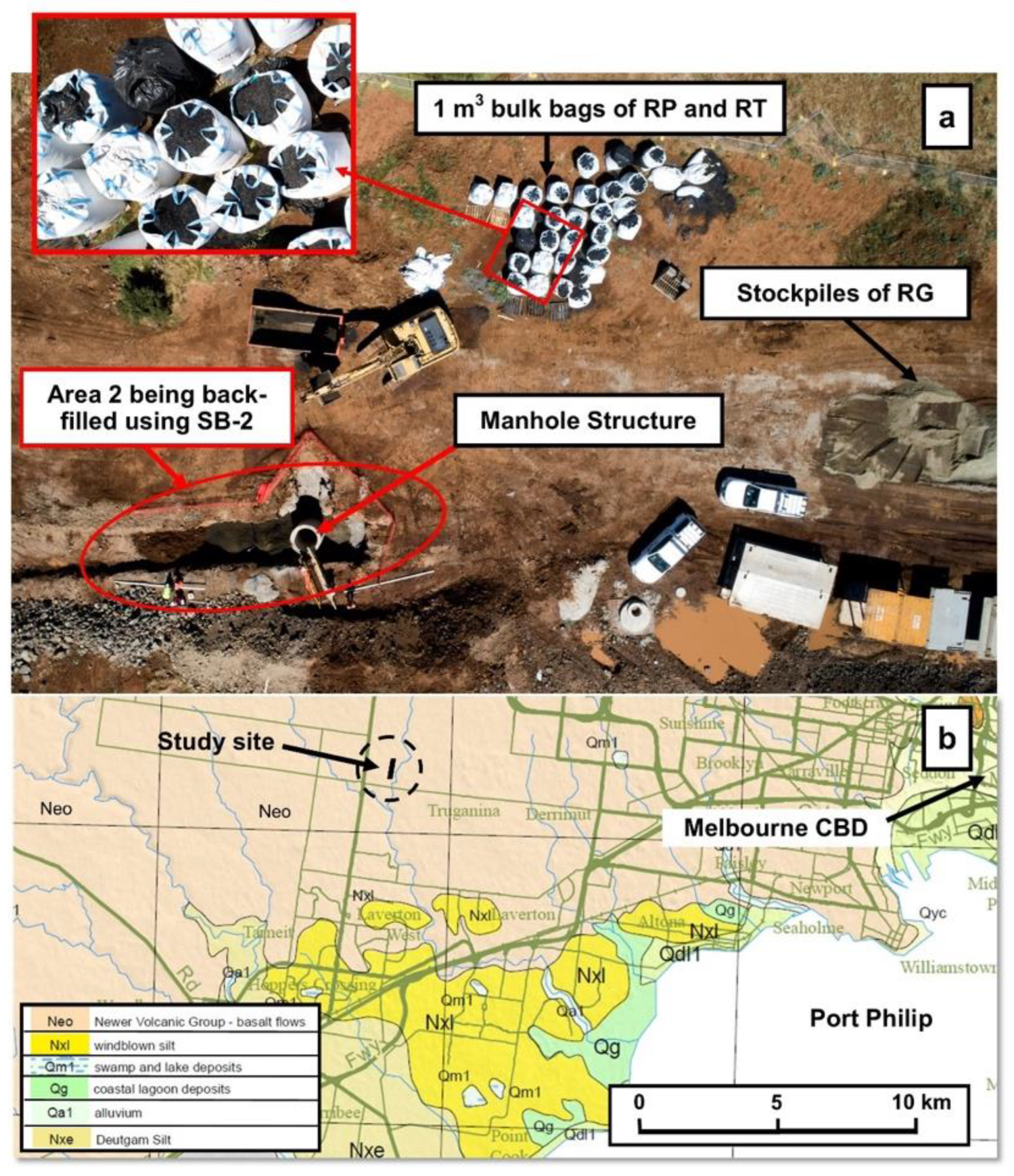
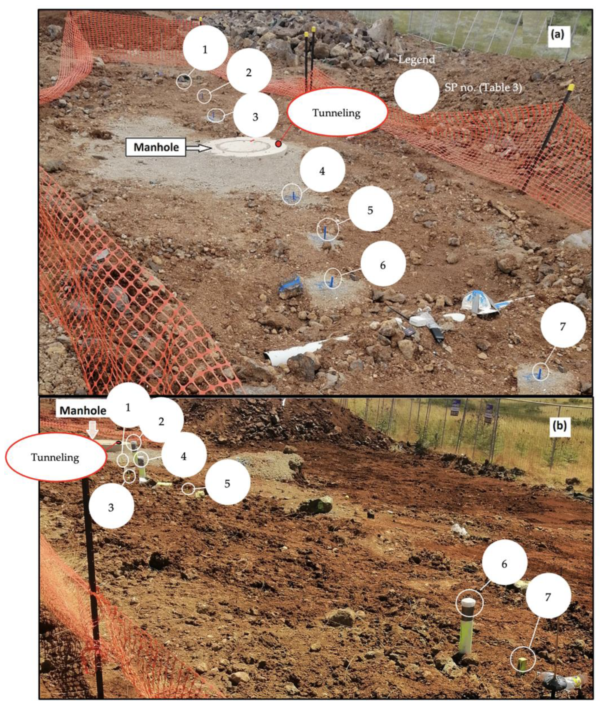
2.1. Summary of Materials, Construction, and Instrumentation

The recycled material blends comprised recycled glass (RG), recycled plastic (RP), and recycled tire (RT) and were supplied by local waste recovery/recycling plants in Victoria, Australia. Figure 1 demonstrates a geological map of the west of Melbourne indicating the study site and the materials transported to the site location for mixing and backfilling the selected areas.

Before the construction stage, several mixtures of RG, RP, and RT were prepared and investigated through extensive environmental and geotechnical testing programs, the details of which can be found in [15]. Two optimum mix designs, labeled SB-1 and SB-2 with (RG:RP:RT) content of (77:09:14) and (84:05:11), respectively, were proposed for the construction of the full-scale trials. The physical properties of SB-1 and SB-2 are presented in

Table 1. Physical properties of SB-1 and SB-2 blends.

Material		SB-1	SB-2	Specification
RG:RP:RT content (% by mass)		77:09:14	84:05:11	--
Particle composition (%)	>4.75 mm	29	22	ASTM-D422 (2007) [30]
	4.75–0.075 mm	69	76
	<0.075 mm	2	2
Maximum particle size (Dmax), mm		19.0	19.0	--
Specific gravity (Gs)		1.93	2.07	ASTM-C127 (2012) [31]
Coefficient of uniformity (Cu)		10.00	9.06
Coefficient of curvature (Cc)		1.49	1.30
USCS classification		SW	SW	ASTM-D2487 (2011) [32]
Standard Proctor compaction	OMC (%)	9.50	7.9	ASTM-D698 (2012) [33]
	MDD (kN/m3)	1.36	1.37

USCS: Unified soil classification system; SW: well-graded sand.

. These blends exhibited a relative density greater than 80% and also showed the least compressibility when undergoing the estimated surcharges of real-life applications (i.e., up to 200 kPa). Relative densities over 80% were reported to correlate with relative compaction greater than 90% [27,28], which is typically the minimum required density for fill earthworks [29].

The natural soil available on the construction site was classified as reactive soil (RS) with high plasticity (CH) after a series of laboratory testing as presented in

Table 2. Physical properties of RS.

Soil Property	Value	Specification
Specific gravity Gs	2.71	ASTM-D854 (2010) [34]
Sand (4.75–0.075) mm	3	ASTM-D422 (2007) [30]
Fine content (<0.075 mm)	97
Liquid limit (LL) (%)	61	ASTM-D4318 (2017) [35]
Plastic limit (PL) (%)	30
Plasticity index (PI) (%)	31
USCS classification	CH	ASTM-D2487 (2011) [32]

.

In the sections selected for the test areas, a 1.5–2 m wide trench was excavated to bury the sewer pipelines and the width of the excavation around the manhole structure of 1.5 m diameter was approximately 1 m, as per the contractor’s construction plan. The depth of the excavation was 3.5 m in test Area 1 and 4.5 m in test Area 2. The sewer pipe was placed within the bottom 1 m of the trench known as the embedment zone and was encapsulated with the standard crushed rock as specified by Melbourne Retail Water Agencies (MRWA) [36]. The test areas were backfilled to 2 m and 3 m above the embedment zone with SB-1 (Area 1) and SB-2 (Area 2), respectively. The top 0.5 m was backfilled with available natural soils of the site for future landscaping purposes. The RS of the site for backfilling consisted of clay with traces of gravel. Up to about 6 and 12 m lengths of the trenches were backfilled using SB-1 and SB-2, respectively, while the rest of the trench was backfilled with RS as per the normal practice, which was considered the benchmark area. More construction details can be found in [16]. The RS used for backfilling in areas 1 and 2 of the trenches are referred to as RS-1 and RS-2, respectively, hereafter.

In both areas 1 and 2, settlement plates (SPs), each comprising a rod and a steel plate were installed. The rods were 15 mm in diameter and 250, 1600, and 3100 mm in length. The dimensions of the steel plate were 200 × 200 × 10 mm (width × length × thickness). During the construction, settlement plates were installed at an appropriate depth and about 100 mm of the rod was left above the ground surface to allow the settlement monitoring using surveying techniques. The SPs in Area 1 were installed at a depth of 0.2 m from the ground surface. In Area 2, the SPs were installed at depths of 0.2, 1.5, and 3 m to investigate the change in settlement with depth, as well as the surface. The SPs in the benchmark site were installed at depths of 0.2 and 1.5 m. The locations of the SPs in areas 1 and 2 are illustrated in Figure 2 and

Table 3. SP distribution in Area 1 and Area 2.

SP No.	Area 1			Area 2
	Depth (m)	Distance * (m)	Material	Depth (m)	Distance * (m)	Material
1	0.2	5.36	RS-1	0.2	1.50	SB-2
2	0.2	3.25	RS-1	3.0	2.50	SB-2
3	0.2	2.13	RS-1	0.2	3.25	SB-2
4	0.2	1.82	SB-1	1.5	4.00	SB-2
5	0.2	2.92	SB-1	0.2	5.50	SB-2
6	0.2	3.84	SB-1	1.5	16.75	RS-2
7	0.2	6.50	RS-1	0.2	18.25	RS-2

* Distance from a particular SP to the manhole center.

.

The deformation monitoring using surveying techniques was carried out from 1 October 2020 to 15 February 2022 for Area 1, and from 26 November 2020 to 15 February 2022 for Area 2. The readings were recorded once a week during the first month after installation to capture potentially frequent early deformations, followed by monthly readings.

2.2. Satellite Data

The European Space Agency (ESA) provides a global SAR dataset from the Sentinel-1 (S-1) mission [37]. This mission is a constellation of two SAR satellites (S-1A and S-1B) carrying C-band instruments with 5.405 GHz. Interferometric wide (IW) swaths with a single look complex (SLC) are used with terrain observation with progressive scans (TOPS) in azimuth for DInSAR, PSI, and SBAS analyses. The S-1 products offer a large swath width of up to 5 by 20 m spatial resolution [38]. S-1A descending data were used in this study with an average 12-day repeat orbit cycle for each satellite and vertical transmission and vertical reception (VV) polarimetric configuration. The S-1A data sensed between October 2020 and February 2022 were analyzed to calculate the ground movement of reactive soil in the west Metro Melbourne, Victoria, Australia, as shown in Figure 1. The S-1A products were from path 118 and frame 719 in sub-swath IW2.

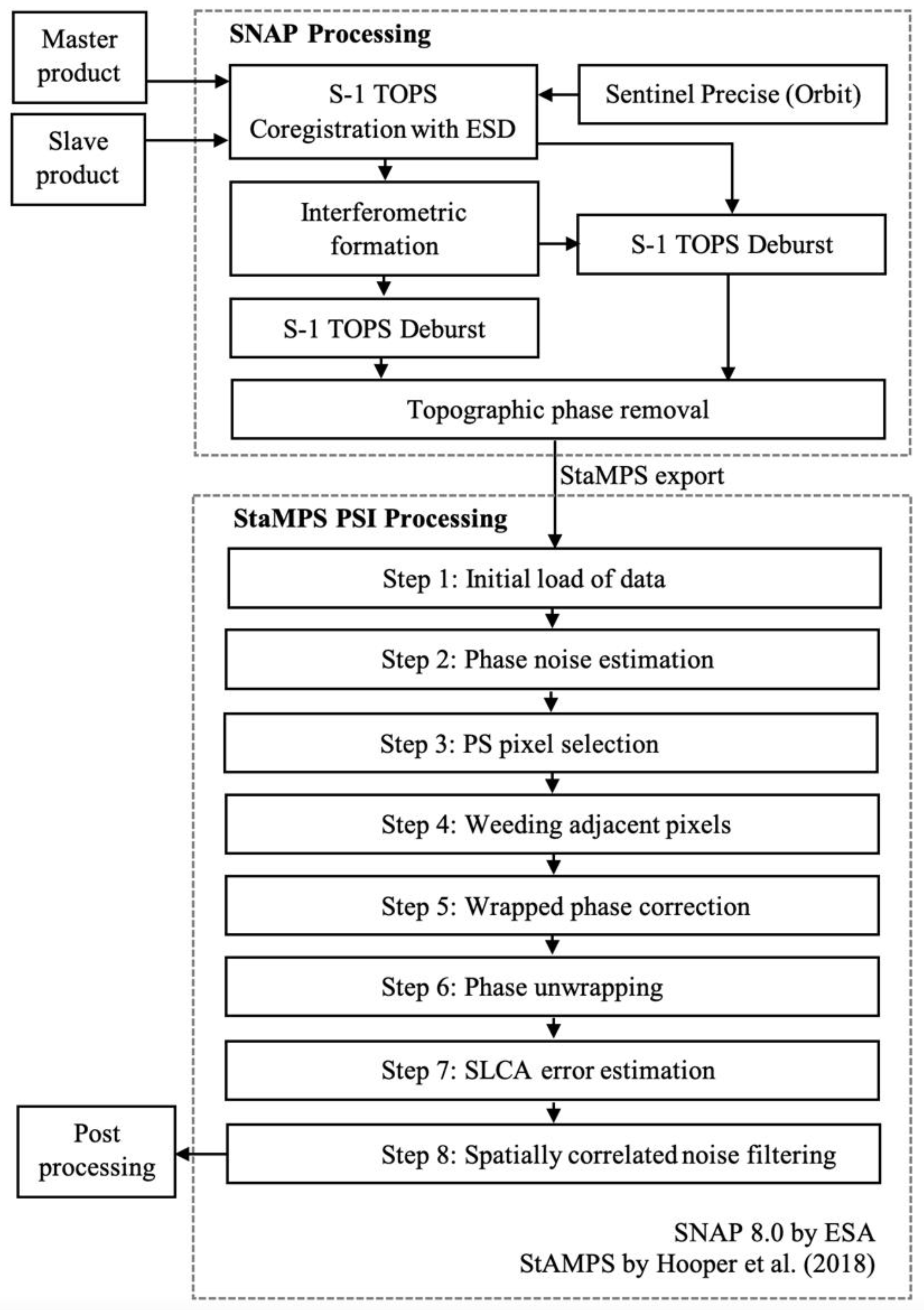
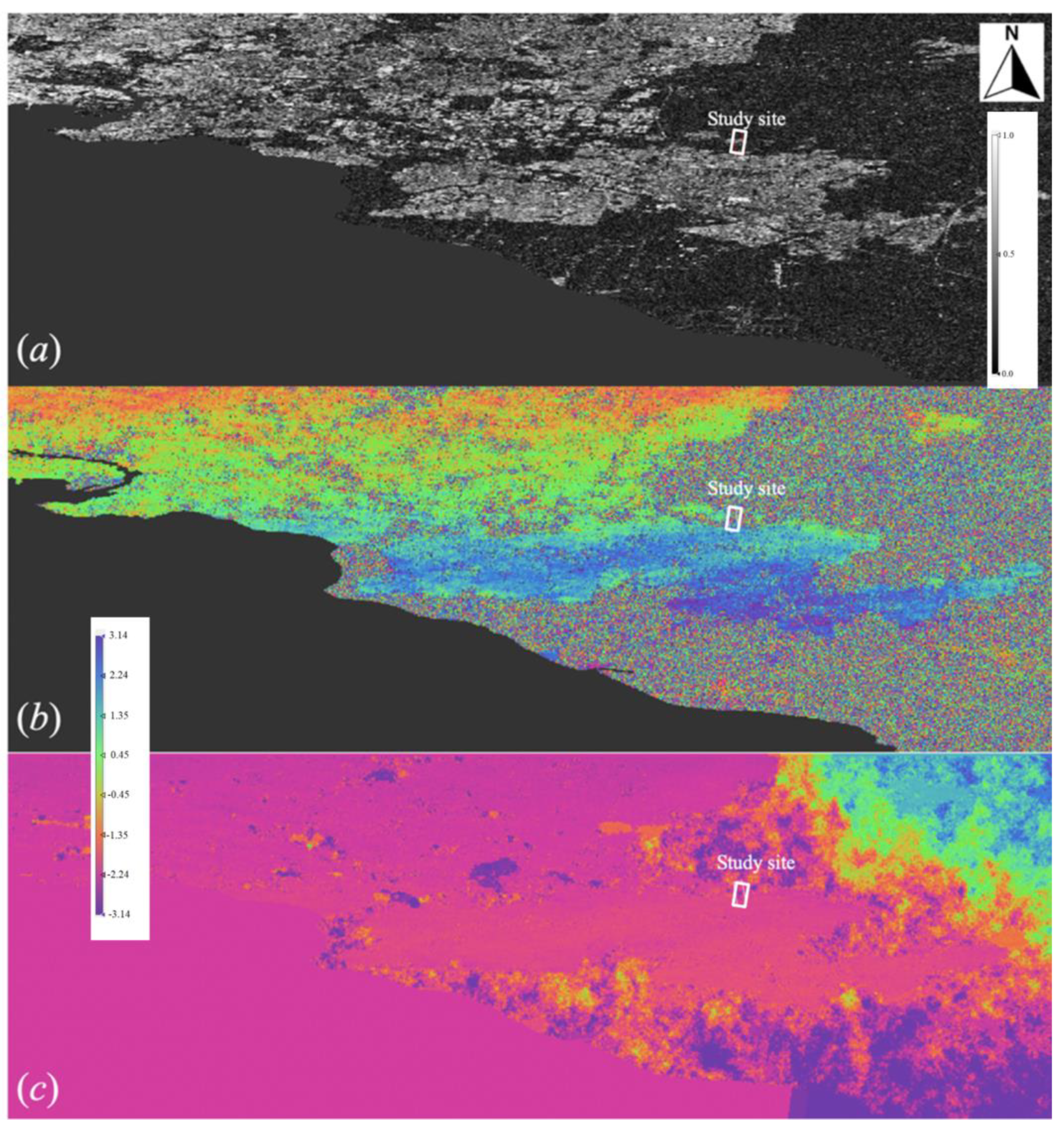
2.3. Satellite Imaging and Analysis

Interferometric SAR (InSAR) uses the phase difference between two or more complex SAR acquisitions of the same area taken from almost similar satellite positions [39]. This can be used to measure changes in the Earth’s surface topography and deformation from geohazard events by setting one image as master and the other as slave. An interferogram (I) is generated through the multiplication of the values of A described as:

$$I=A_r{A}_{\mathrm{s}}{e}^{i\left({\phi }_{\mathrm{m}}-{\phi }_{\mathrm{s}}\right)}={\phi }_{topo}+{\phi }_{defo}+{\phi }_{flat}+{\phi }_{atm}+{\phi }_{noise},$$

(1)

where A_r and A_s are the amplitudes for the reference and secondary SAR images, φ_r and φ_s are the phase information for the reference and secondary SAR images, respectively, φ_topo is the topographic phase, φ_defo is the phase contribution due to surface deformation, φ_flat is the flat-earth phase, φ_atm is the atmospheric phase and φ_noise is the noise-related phase. The value of φ_r can be estimated as:

$${\phi }_r=-\frac{4\pi }{\lambda }{R}_1+{\phi }_{\mathrm{scatt}-1},$$

(2)

where R₁ is the range distance between the location of the reference SAR image and the target surface, and φ_scatt−1 is the backscattering property at the first acquisition time. Similarly, the secondary SAR image φ_s can be calculated as:

$${\phi }_{\mathrm{s}}=-\frac{4\pi }{\lambda }(R_2)+{\phi }_{\mathrm{scatt}-2}=-\frac{4\pi }{\lambda }(R_1+\mathsf{\Delta }R)+{\phi }_{\mathrm{scatt}-2},$$

(3)

where R₂ is the range distance between the location of the secondary SAR image and the target surface and φ_scatt−2 is the backscattering property at the second acquisition time. The value of R₂ can be substituted by R₁ + ΔR, and the value of ΔR can be estimated as:

$$\Delta R=B_{┴} \tan \left(\alpha \right),$$

(4)

where $B_{┴}$ is the perpendicular baseline between the reference and the secondary SAR images, and the angle α is the angle between $B_{┴}$ and the actual distance between the reference and the secondary SAR images. Assuming that there is a constant backscattering property for the targeted surface, φ_scatt−1 and φ_scatt−2 can also be assumed to have similar values. Hence, the interferometric phase can be described as [17]:

$${\phi }_r-{\phi }_{\mathrm{s}}=\frac{4\pi }{\lambda }\mathsf{\Delta }R.$$

(5)

The interferometric phase, φ_m − φ_s, can be used to estimate the height of the object on the ground. The temporal baseline (B_t), which is the time delay between the reference and the secondary SAR images, is important to consider. This influences the probability of changes in backscattering properties, φ_scatt−1 and φ_scatt−2, primarily due to changes in the land cover or vegetation and wind-induced tree movements [23].

The S-1 data were processed using SNAP 8.0 by ESA with an implemented workflow described in Figure 3. The first stage was the coregistration between the reference and secondary SAR images. The 3-sec digital elevation model (DEM) and the sentinel precise orbit data were implemented in this initial step. The next stage was the interferogram generation between the reference and secondary products, flat-earth subtraction, and coherence (γ) estimation. Topographic phase removal was employed to obtain DInSAR results. The Goldstein phase filtering by [40] for phase noise reduction was then performed. The resulting product was exported for the statistical-cost network-flow algorithm for the phase unwrapping (SNAPHU) [41]. Phase unwrapping with SNAPHU recovers the original phase values by adding appropriate multiples of 2π to each phase input. The result of the unwrapping was imported back to SNAP and then converted to displacements [18].

The PSI processing enables the measurement of surface displacement sub-millimeter accuracy using pixels with a more stable phase called the permanent scatterers [19]. Using the combined SNAP and Stanford method for persistent scatterers (StaMPS) workflow, these scatterers are analyzed as part of the PSI processing as shown in Figure 4. The first stage in PSI processing uses SNAP to determine the reference image using the InSAR stack overview tool. The reference image was selected such that $B_{┴}$ is minimized and the γ of the stack is maximized. The secondary images were then coregistered with the reference image. Interferograms were generated and debursting was conducted. The topographic phase was removed and then the resulting product was exported to a format that is readable by StaMPS. The StaMPS processing has eight steps, as shown in Figure 4. The linear correction of the toolbox for reducing atmospheric InSAR noise (TRAIN) by [41] was used for tropospheric adjustment. The estimated time series displacement (d) and mean annual velocity (v) were then obtained.

The SBAS method is comparable to the PSI method with the key difference in the pairing of InSAR images. The SBAS method produces differential interferograms from all the input InSAR images stacked with varying pairing combinations that fulfil the criteria of temporal and geometric baseline, whilst the PS method assigns one reference InSAR image to be paired with all secondary InSAR images. The SBAS processing using the combined SNAP and StaMPS workflow is shown in Figure 5.

3. Results

3.1. Field Monitoring

Figure 6 shows the displacements measured at settlement plate (SP) locations in areas 1 and 2. The negative and positive values indicate settlement and heaving with respect to the initial position of the SPs, respectively. Figure 6 shows that the maximum ground movements recorded in SB-1 and SB-2 areas were −15 and −17 mm, respectively, whereas for the RS-1 and RS-2, the maximum ground movements detected were −48 mm and −110 mm, respectively, over the 17 months of the monitoring period. This indicates strikingly smaller settlements of SBs compared to the RS backfills (about six times lower). It should be noted that RS-1 and RS-2 movements were different both in the magnitudes and trends, in spite of being the same soil types located close to each other. This was potentially attributed to the poor quality and lack of consistency in compacting clay in deep excavated trenches which is a challenging task. In fact, challenges associated with backfilling deep trenches with site-won clay was the problem [4] tried to resolve by developing blends of recycled materials that exhibited self-compacting properties or at least required less compactive effort to reach the desired density and a more consistent manner along the backfilled trench. Another potential reason for inconsistent settlements in the two areas could be the difference in the drainage that affected the stormwater flow and hence, different deformations on the surface.

The values of the cumulative soil movement of SB and RS in Areas 1 and 2 measured at 0.2 m depth were averaged as shown in Figure 7 for the purpose of fair comparison with the spatial resolution of the satellite image analyses.

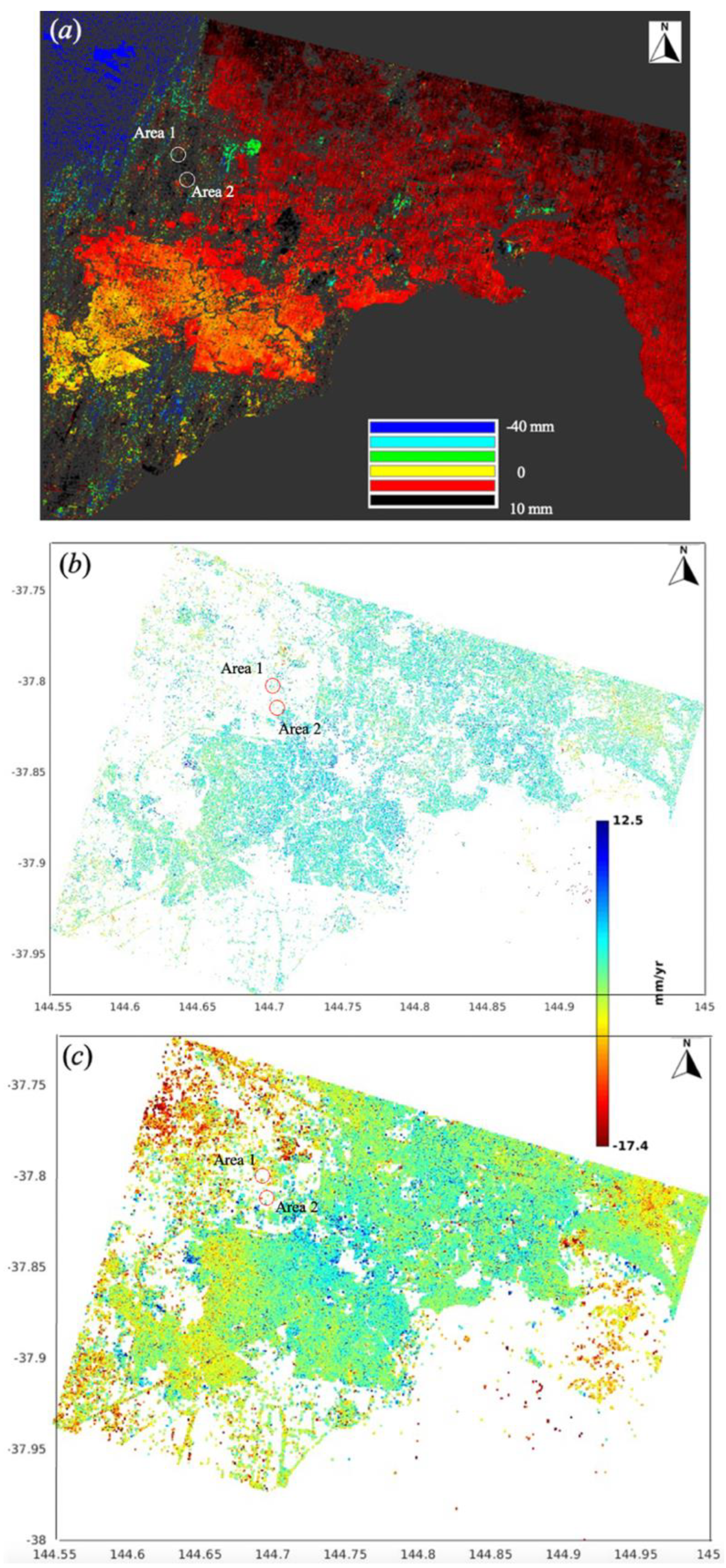
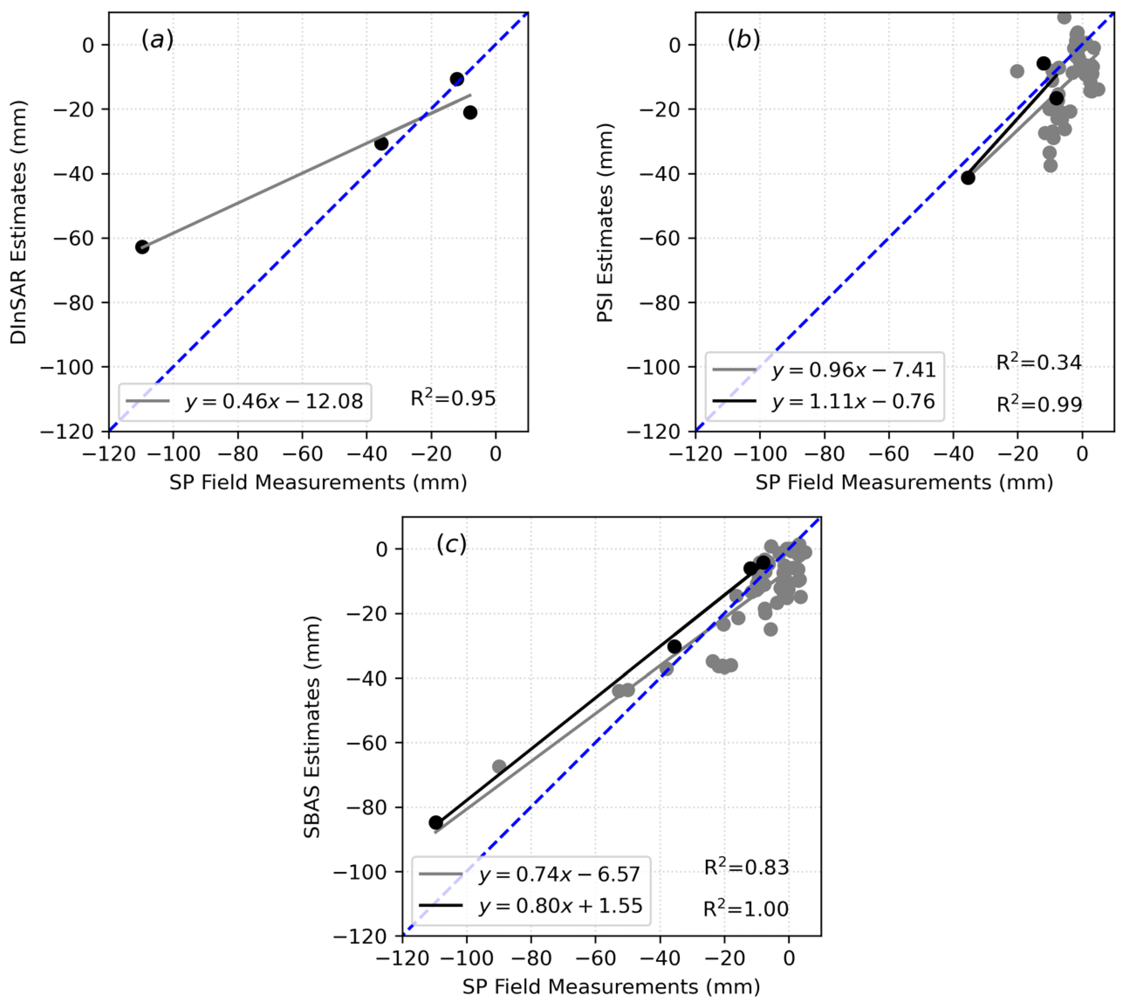
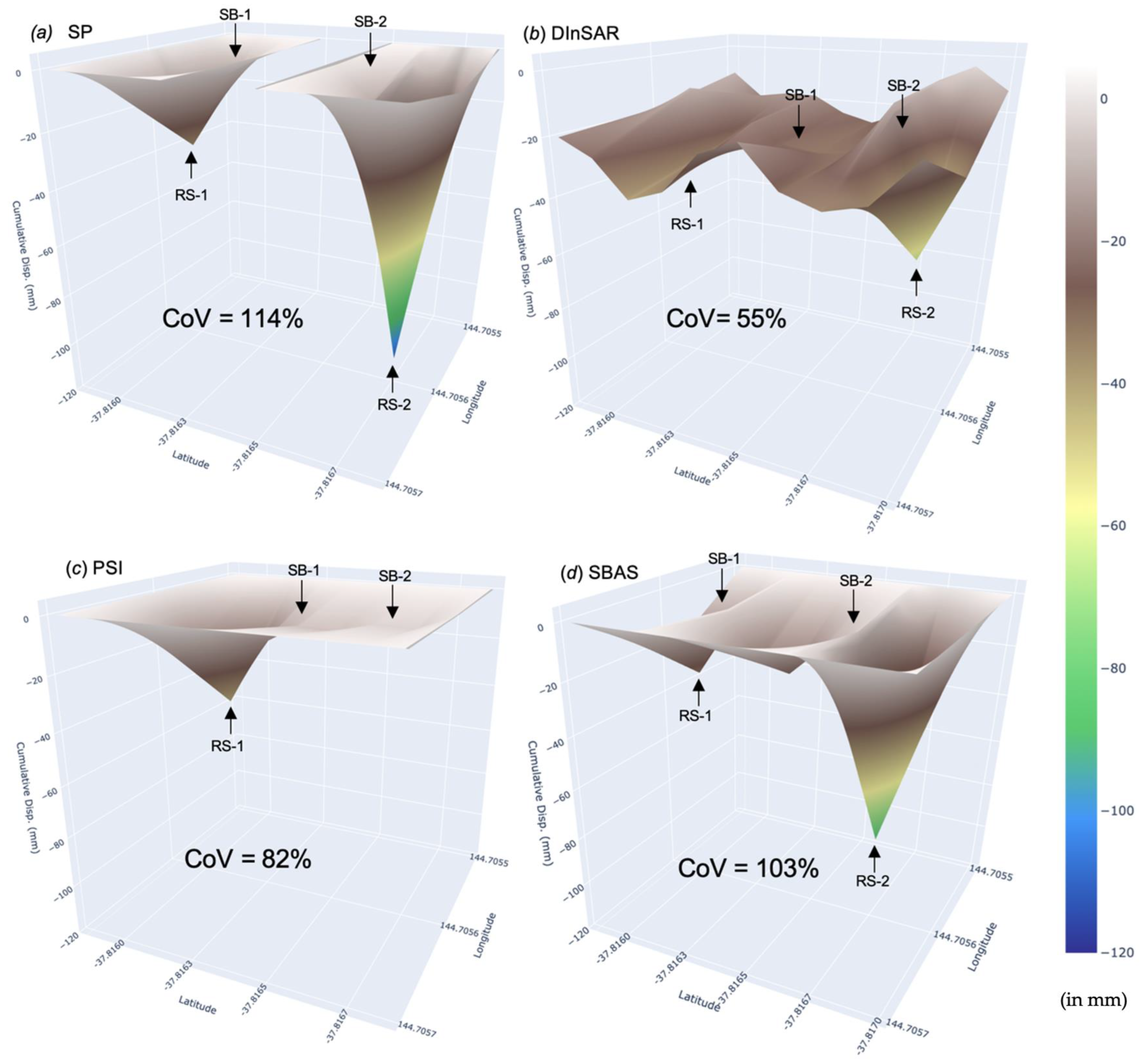
3.2. InSAR Estimates

The ground movements of the trial site of this project were also investigated using InSAR techniques. Sample results of the InSAR analyses showing the coherence, wrapped phase, and unwrapped phase maps are presented in Figure 8.

First, DInSAR was used to estimate the final cumulative estimates of ground movement (Figure 9a). Two S-1A satellite images were used which were sensed on 6 October 2020 and on 25 February 2022 for Area 1. Similarly, two S-1A satellite images were analyzed for Area 2 obtained on 19 November 2020 and on 25 February 2022. The selected satellite images for Area 1 and Area 2 were the closest available sentinel data from the field monitoring commencement and completion dates. This is based on the 12-day orbit cycle of S-1A described in Section 2.2. The difference in the used S-1A satellite images for each area is due to the dissimilar completion of the trench excavation and backfilling in the area. The DInSAR estimates for each location are shown in Figure 10. The results of the DInSAR analysis overestimated the ground movements of SB-1 and SB-2 (Figure 10a,c), whilst underestimating that of RS-1 and RS-2 (Figure 10b,d). The estimated values of the ground movement were −21 and −11 mm for SB-1 and SB-2, respectively. On the other hand, RS-1 and RS-2 observed higher ground movement estimates equal to −31 mm and −63 mm. Despite the difference in magnitudes, the trends of the estimated DInSAR values are comparable to the field measurements using SPs, where lower ground surface movements were recorded in SB than those in RS.

The PSI and SBAS techniques were also performed to estimate the ground movement of the two study areas. These techniques enabled the time-series analysis of S-1A images between 6 October 2020 and 25 February 2022 for Area 1 and between 19 November 2020 and 25 February 2022 for SB-2 for Area 2 (Figure 9b,c).

The results of the PSI analysis are shown in Figure 10 where ground movements of −17, −6, and −41 mm were observed for SB-1 and SB-2, and RS-1, respectively. The pixel for RS-2 exceeded the temporal and baseline limit leading to spatiotemporal decorrelation, which caused the specific persistent scatterer to be disregarded, as shown in Figure 10d. This is a known limitation of the PSI technique, which focuses on scatterers that have defined geometry such as developed or urban environments [43]. This was evident in Figure 9b where limited permanent pixel scatterers were selected. Overall, PSI results are more comparable to field measurements than those of DInSAR.

The SBAS analysis estimated ground movements of −4 and −6 mm for SB-1 and SB-2, and −30 and −85 mm for RS-1 and RS-2, respectively. These results had the closest values to the SP field measurements, except for SB-2. The better accuracy can be attributed to the fact that the SBAS technique is more reliable in areas without well-defined geometry such as vegetation and open fields [44]. This is due to the ability of the SBAS analysis to consider small temporal baselines and backscattered signals of distributed scatterers reducing the influence of the spatiotemporal decorrelation [45].

4. Discussions

4.1. Comparison between the Field Monitoring and InSAR Analysis

The accuracy of the methods used, namely SP field measurements and InSAR techniques, to investigate the performance of the two adjacent areas with SBs and RS were compared in Figure 11. This helped to assess the reliability of each method and understanding their limitations. It is important to note that for the DInSAR estimates, only the magnitude of the final ground movement can be estimated. This is reflected in Figure 11a with only four points showing the estimated values for the four areas, SB-1, SB-2, RS-1, and RS-2. Conversely, PSI and SBAS techniques are time-series InSAR analyses that can capture the temporal changes of ground movements represented by the data points in Figure 11b,c.

In general, the results of the comparison using scatter plots between the measured SP and InSAR estimates suggested an acceptable regression coefficient. The DInSAR estimates were observed to have the lowest regression coefficient equivalent to 0.46 (Figure 11a). It can be observed that there are three distinguishable regions of the comparison in Figure 11a. The first subsection is where the value of the ground movement is less than −50 mm. Within this zone, the DInSAR estimate seems to underestimate the measured SP values. The second subsection is between −50 and −30 mm, where the DInSAR estimate obtained comparable values with the SP field measurement. Lastly, the third zone is where the values of the ground movement are greater than −30 mm. Within this zone, the ground movement values obtained in the field using SP were slightly overestimated. The scatterplot of the data points was not dispersed due to the limited number of points being compared. This led to a high calculated value of R² being 0.95. However, the calculated root mean square error (RMSE) between the DInSAR estimates and the collected SP data was exorbitant, equal to 24.47.

The comparative analysis between the PSI estimates and the measured SP field data was divided into two, as presented in Figure 11b. The comparative analysis for RS-2 was neglected due to the spatiotemporal decorrelation of the pixel where it is located. The first comparison was between the final cumulative values of the ground movement. The accuracy of the result of this analysis surpassed that of the DInSAR and SP comparison. The regression coefficient of the final cumulative values of the ground movement between PSI and SP was 1.11. It can be observed in Figure 11b that the PSI technique overestimated the final values of the ground movement in comparison with the measured SP data. The calculated value of R² was 0.99 and this closer to the unity value may have been influenced by the limited available data points, similar to the previous DInSAR and SP comparison. However, the value of the calculated RMSE was half of the DInSAR and SP comparison, which was equal to 7.02. The second PSI and SP comparison considered all the time-series data points (Figure 11b). When all the time-series data points were considered, the regression coefficient remained acceptable equaling 0.96 with the PSI values overestimating the SP data. Conversely, the value of R² significantly decreased from 0.99 to 0.34, showing the overall dataset’s high dispersion. Similarly, the value of RMSE was negatively influenced by considering all the data points, increasing from 6.04 to 11.34. This value was comparable to the RMSE value calculated from the DInSAR and SP comparison.

The comparison between the SBAS estimates and the measured SP field data led to an acceptable match for both the final cumulative values of the ground movement and all the time-series data points (Figure 11c). The accuracy of the result of the final cumulative values was analogous to the results of the PSI and SP comparison. The regression coefficient of the final cumulative values of the ground movement between SBAS and SP was 0.80 and the calculated value of R² was 1.00. However, the value of the calculated RMSE was almost twice that of the PSI and SP comparison, which was equal to 13.20 with consideration of RS-2. When all the time-series data points were considered, the regression coefficient remained acceptable equal to 0.74. Conversely, the value of R² decreased from 1.00 to 0.83, which is still an acceptable value with the SBAS values overestimating the SP data. The value of RMSE decreased from 13.20 to 9.26.

4.2. Temporal Variation

The values of the coefficient of variation (CoV), which is the ratio of the standard deviation to the mean, of the temporal measurements of SPs and estimates of PSI, and SBAS were calculated to demonstrate the extent of variability of the ground movement values within SB and RS areas. The calculated values of CoV will allow the determination of the temporal volatility or risk associated when using SP field data and InSAR estimates. The temporal variation of the measurements using SP and estimates using PSI and SBAS varied depending on the magnitude of the ground movement, as depicted in Figure 12. Due to the small values of recorded ground movements, the earlier monitored and estimated values of ground movement closer to the commencement date of the study around 1 November 2020 for Area 1 and 3 December 2020 for Area 2 exhibited high values of CoV.

The surface movement of SB-1 in Figure 12a calculated consistently high values of CoV with an average of 170%. The most volatile measurements and calculations were obtained on 13 July 2021 equal to a CoV of 490%, whilst the most stable was the values of final cumulative ground movement on 15 February 2022 with a CoV of 70%. Similarly in SB-2 (Figure 12b), the calculated values of CoV were constantly high with an average of around 100%. The highest CoV was on 3 December 2021 equivalent to 450%, whilst the lowest was obtained on 22 June 2021 approximately 10%. It can be observed that the temporal values of CoV were generally higher in areas with constructed SB due to lower magnitudes of ground surface movements.

In the locations with RS, the calculated values of CoV were relatively lower compared to that with SB. This is due to the higher magnitudes of the measured and estimated ground surface movements in RS-1 and RS-2 (Figure 12c,d). The average values of CoV for RS-1 and RS-2 were around 130% and 40%, respectively. Due to the similar reason of having ground movement values close to zero, the earlier monitored and estimated values of ground movement closer to the commencement date of the study from 1 November 2020 for Area 1 and from 3 December 2020 for Area 2 exhibited high values of CoV. After the early investigation stage, the CoV values were consistently low reaching values close to 1% for both RS-1 and RS-2 around the final stage. Overall, the temporal volatility of ground movement values, either measured or estimated, was lowest in RS-2.

4.3. Spatiotemporal Variation

The spatial variation of the final ground movement along the entire strip covering the areas of interest is shown in Figure 13. This displays the difference in the measured SP data and the estimates of DInSAR, PSI, and SBAS. The graph in Figure 13a that shows the averaged SP measurements were noticeably dissimilar from the topographic features of DInSAR in Figure 13b. On the other hand, both PSI (Figure 13c) and SBAS (Figure 13d) considerably contained similar features to the SP topography (Figure 13a). It can be observed that Area 1 (both SB-1 and RS-1) in Figure 13c closely resembles the variations in Figure 13a. However, the pixel for RS-2 in the PSI analysis was neglected which affected the graph and CoV calculation. In the SBAS analysis in Figure 13d, the SB and RS locations were the closest resemblances to the SP measurements plotted in Figure 13a. Noting that, the averaged measurements of SP between SB-1 and SB-2 were not available to compare with the SBAS pixel estimates.

To investigate the spatiotemporal variation of the measured SP and the estimated InSAR values, the spatial CoV of the cumulative ground movement of the whole study site strip, Area 1, and Area 2 (described in Figure 1 and Figure 2) were calculated for the early stage (between October 2020 and December 2020), the middle stage (between October 2020 and April 2021), and the final stage (between October 2020 and February 2022) of the investigation. The spatiotemporal variation, reflected by the CoV values of the measured SP and the estimated DInSAR, PSI, and SBAS estimates, are listed in

Table 4. Spatiotemporal comparison between SP measurements and InSAR estimates in the early (between October 2020 and December 2020), middle (between October 2020 and April 2021), and final stages (between October 2020 and February 2022).

Coefficient of Variation, CoV, in %
Method	Early CoV (%)			Middle CoV (%)			Final CoV (%)
	Whole Strip	Area 1	Area 2	Whole Strip	Area 1	Area 2	Whole Strip	Area 1	Area 2
SP	162	37	16	132	97	109	114	90	113
DInSAR	76	77	26	74	201	11	55	19	75
PSI	151	50	-	79	73	-	82	76	-
SBAS	109	14	34	61	11	73	103	71	90
Minimum Value in mm
Method	Early Min Value (mm)			Middle Min Value (mm)			Final Min Value (mm)
	Whole Strip	Area 1	Area 2	Whole Strip	Area 1	Area 2	Whole Strip	Area 1	Area 2
SP	−0.63	2.90	−0.63	−49.97	−9.47	−49.97	−109.60	−35.51	−109.60
DInSAR	1.94	1.94	13.38	−0.36	0.36	5.28	−62.70	−30.70	−62.70
PSI	−13.84	−13.84	-	−33.58	−33.58	-	−41.35	−41.35	-
SBAS	−11.80	−1.87	−11.80	−36.35	−13.74	−36.35	−84.75	−30.17	−84.75
Maximum value in mm
Method	Early Max Value (mm)			Middle Max Value (mm)			Final Max Value (mm)
	Whole Strip	Area 1	Area 2	Whole Strip	Area 1	Area 2	Whole Strip	Area 1	Area 2
SP	4.93	4.93	−0.50	−1.76	−1.76	−6.49	−7.97	−7.97	−12.00
DInSAR	27.01	6.62	19.42	6.19	5.99	6.19	−10.56	−21.01	−10.56
PSI	2.89	−4.56	-	−0.60	−3.69	-	−5.80	−8.90	-
SBAS	0.85	−1.44	−5.74	−9.72	−11.00	−11.03	−4.15	−4.15	−6.01

.

In the early stage, the calculated values of CoV in the whole strip were high, ranging from 76% to 162%. These values show that the initial cumulative surface ground movement of Area 1 and Area 2 was different may be due to the heterogeneity of the soil in the study site, the drainage affecting the stormwater flow, or lack of consistency in the backfilling construction, especially for RS-1 and RS-2. Considering only Area 1, the measurements and estimates of SP and InSAR analyses varied. In Table 4, the CoV values of SP and SBAS were lower than the CoV values of DInSAR and PSI. This signifies that the variability of the values of the measurements and estimates by SP and SBAS between SB-1 and RS-1 was low in the early stage. On the contrary, the CoV of DInSAR and PSI started with high values denoting a great difference in values between SB-1 and RS-1. In Area 2, the values of CoV for the SP measurements were approximately twice that of the DInSAR and SBAS. This means that the difference in the actual early cumulative ground movement of SP between SB-2 and RS-2 was supposed to be higher than the estimations of DInSAR and SBAS.

In the middle stage, the CoV values of InSAR analyses were half of the measured SP data of the entire study site. In Area 1, the values of CoV varied from 11% to 201% estimated by SBAS and DInSAR, respectively. Similarly, the values of CoV had a wide range from 11% to 109% estimated and measured by DInSAR and SP, respectively. The CoV values for SP in the whole strip, Area 1, and Area 2 were consistently around 100%.

In the final stage, the values of CoV for SP and SBAS for the whole study site, Area 1, and Area 2 were comparable. On the other hand, the CoV values of DInSAR had the most diverged estimate. This reflects that the level of variation between SB and RS in the measured SP data was corresponding to the SBAS estimates. Hence, this generally captures acceptable cumulative ground movement magnitude influenced by spatiotemporal stabilization of the constructed SB in both Area 1 and Area 2.

In summary, the spatiotemporal variation of the measured data using SP was closest to the spatiotemporal values of CoV estimated using SBAS. This method is reliable in areas without well-defined geometry affected by seasonal-dependent growth and withering of vegetation and open fields influenced by climate–crop interactions [44]. The SBAS analysis considers small temporal baselines and backscattered signals of distributed scatterers that reduce the influence of the spatiotemporal decorrelation [45]. Due to this, SBAS estimates had the closest values and spatiotemporal variation to the measured SP field data, with consideration of the SB and RS zones.

5. Conclusions

The spatiotemporal performance of sustainable backfill materials made of recycled aggregates, as alternative construction materials for sewage pipeline trenches, was investigated in a highly reactive soil area. The investigation involved two different blends of sustainable backfills (SB) comprised of 100% recycled aggregates that were utilized as backfill materials for deep excavated trenches in Western Melbourne. Two adjacent trial sites were constructed using the proposed SBs of this study and were monitored for deformations using settlement plates (SP) and surveying techniques. InSAR techniques, DInSAR, PSI, and SBAS, were implemented to assess the deformation performance of the two adjacent SBs and their influence on the surrounding areas. This investigation resulted in a deeper understanding of the deformation behavior of the adjacent study areas backfilled with SB and with the site’s reactive soils (RS). The results of the InSAR estimates were correlated with the measured SP field data to determine the accuracy of the estimations. The estimated ground movement using InSAR analysis captured the spatial difference between the SB and RS zones in Area 1 and Area 2. In Area 1, the magnitudes of the ground movement were twice the values measured in Area 2. This was consistently identified in the InSAR analyses. Moreover, the differences in the ground movement between SB-1 and RS-1, and between SB-2 and RS-2, were also adequately captured by the DInSAR, PSI, and SBAS estimates.

The comparison between the measured SP and InSAR estimates generally had acceptable results. The DInSAR estimations least matched the measured SP field data, while the PSI estimations obtained better accuracy than the DInSAR values. However, the pixel for RS-2 was neglected in the PSI analysis, since it focuses on scatterers that have defined geometry and built-up areas. The SBAS estimates were found to have the most accurate results. Similarly, the values of CoV (coefficient of variation) showing the spatial and temporal difference in the SB and RS zones of the study site of the measured SP data were by the SBAS estimations. This method was observed to be the most reliable among the InSAR methods used in this study. Thus, it can be deduced that for environments without well-defined and changing features, such as SB and RS surfaces, SBAS can be reliably used for spatiotemporal analysis.

This study provided a novel approach for evaluating the performance of blends of recycled aggregates as alternative backfill materials to promote their global applicability to be used in highly reactive sites considering the spatiotemporal impact. This approach is useful for complementing the limited field monitoring instrumentation to extrapolate spatial and temporal analyses.

References

1. Fityus, S.G.; Smith, D.W.; Allman, M.A. Expansive Soil Test Site near Newcastle. J. Geotech. Geoenviron. Eng. 2004, 130, 686–695. [Google Scholar] [CrossRef]
2. Li, J.; Cameron, D.A.; Ren, G. Case Study and Back Analysis of a Residential Building Damaged by Expansive Soils. Comput. Geotech. 2014, 56, 89–99. [Google Scholar] [CrossRef] [Green Version]
3. Rajeev, P.; Kodikara, J. Numerical Analysis of an Experimental Pipe Buried in Swelling Soil. Comput. Geotech. 2011, 38, 897–904. [Google Scholar] [CrossRef]
4. Water Services Association of Australia. WSA Conduit Inspection Reporting Code of Australia Version 2.2; Water Services Association of Australia: Docklands, VIC, Australia, 2008. [Google Scholar]
5. Karunarathne, A.M.A.N.; Gad, E.F.; Rajeev, P. Effect of Insitu Moisture Content in Shrink-Swell Index. Geotech. Geol. Eng. 2020, 38, 6385–6392. [Google Scholar] [CrossRef]
6. Richards, R.A. Should Selection for Yield in Saline Regions Be Made on Saline or Non-Saline Soils? Euphytica 1983, 32, 431–438. [Google Scholar] [CrossRef]
7. Gedara, S.D.D.A.; Wasantha, P.L.P.; Teodosio, B.; Li, J. An Experimental Study of the Size Effect on Core Shrinkage Behaviour of Reactive Soils. Transp. Geotech. 2022, 33, 100709. [Google Scholar] [CrossRef]
8. Tran, K.M.; Bui, H.H.; Sánchez, M.; Kodikara, J. A DEM Approach to Study Desiccation Processes in Slurry Soils. Comput. Geotech. 2020, 120, 103448. [Google Scholar] [CrossRef]
9. Tran, K.M.; Bui, H.H.; Nguyen, G.D. A Hybrid Discrete-Continuum Approach to Model Hydro-Mechanical Behaviour of Soil during Desiccation. arXiv 2021, arXiv:2106.04676. [Google Scholar]
10. Gandini, A.; Quesada, L.; Prieto, I.; Garmendia, L. Climate Change Risk Assessment: A Holistic Multi-Stakeholder Methodology for the Sustainable Development of Cities. Sustain. Cities Soc. 2021, 65, 102641. [Google Scholar] [CrossRef]
11. Uchehara, I.; Moore, D.; Jafarifar, N.; Omotayo, T. Sustainability Rating System for Highway Design—A Key Focus for Developing Sustainable Cities and Societies in Nigeria. Sustain. Cities Soc. 2022, 78, 103620. [Google Scholar] [CrossRef]
12. Fauzi, A.; Djauhari, Z.; Juniansyah Fauzi, U. Soil Engineering Properties Improvement by Utilization of Cut Waste Plastic and Crushed Waste Glass as Additive. Int. J. Eng. Technol. 2016, 8, 15–18. [Google Scholar] [CrossRef]
13. Imteaz, M.A.; Arulrajah, A.; Horpibulsuk, S.; Ahsan, A. Environmental Suitability and Carbon Footprint Savings of Recycled Tyre Crumbs for Road Applications. Int. J. Environ. Res. 2018, 12, 693–702. [Google Scholar] [CrossRef]
14. Yaghoubi, E.; Yaghoubi, M.; Guerrieri, M.; Sudarsanan, N. Improving Expansive Clay Subgrades Using Recycled Glass: Resilient Modulus Characteristics and Pavement Performance. Constr. Build. Mater. 2021, 302, 124384. [Google Scholar] [CrossRef]
15. Yaghoubi, E.; Al-Taie, A.; Disfani, M.; Fragomeni, S. Recycled Aggregate Mixtures for Backfilling Sewer Trenches in Nontrafficable Areas. Int. J. Geomech. 2022, 22, 04021308. [Google Scholar] [CrossRef]
16. Al-Taie, A.; Yaghoubi, E.; Disfani, M.; Fragomeni, S.; Gmehling, E. Field Performance Evaluation of Recycled Aggregate Blends Used for Backfilling Deep Excavated Trenches. Int. J. Geomech. 2022. Revised in 2022. [Google Scholar]
17. Plank, S. Rapid Damage Assessment by Means of Multi-Temporal SAR—A Comprehensive Review and Outlook to Sentinel-1. Remote. Sens. 2014, 6, 4870–4906. [Google Scholar] [CrossRef] [Green Version]
18. European Space Agency. European Space Agency Sentinel-1 SAR User Guide; European Space Agency: Paris, France, 2020. [Google Scholar]
19. Crosetto, M.; Monserrat, O.; Cuevas-González, M.; Devanthéry, N.; Crippa, B. Persistent Scatterer Interferometry: A Review. ISPRS J. Photogramm. Remote. Sens. 2016, 115, 78–89. [Google Scholar] [CrossRef] [Green Version]
20. Lu, P.; Bai, S.; Tofani, V.; Casagli, N. Landslides Detection through Optimized Hot Spot Analysis on Persistent Scatterers and Distributed Scatterers. ISPRS J. Photogramm. Remote. Sens. 2019, 156, 147–159. [Google Scholar] [CrossRef]
21. Schlögl, M.; Widhalm, B.; Avian, M. Comprehensive Time-Series Analysis of Bridge Deformation Using Differential Satellite Radar Interferometry Based on Sentinel-1. ISPRS J. Photogramm. Remote Sens. 2021, 172, 132–146. [Google Scholar] [CrossRef]
22. Johnston, P.J.; Filmer, M.S.; Fuhrmann, T. Evaluation of Methods for Connecting InSAR to a Terrestrial Reference Frame in the Latrobe Valley, Australia. J. Geod. 2021, 95, 115. [Google Scholar] [CrossRef]
23. Teodosio, B.; Wasantha, P.L.P.; Yaghoubi, E.; Guerrieri, M.; Fragomeni, S.; van Staden, R.C. Monitoring of Geohazards Using Differential Interferometric Satellite Aperture Radar in Australia. Int. J. Remote Sens. 2022, 43, 3769–3802. [Google Scholar] [CrossRef]
24. Parker, A.L.; Castellazzi, P.; Fuhrmann, T.; Garthwaite, M.C.; Featherstone, W.E. Applications of Satellite Radar Imagery for Hazard Monitoring: Insights from Australia. Remote. Sens. 2021, 13, 1422. [Google Scholar] [CrossRef]
25. Du, Z.; Ge, L.; Li, X.; Ng, A. Subsidence Monitoring over the Southern Coalfield, Australia Using Both L-Band and C-Band SAR Time Series Analysis. Remote. Sens. 2016, 8, 543. [Google Scholar] [CrossRef] [Green Version]
26. De Novellis, V.; Atzori, S.; De Luca, C.; Manzo, M.; Valerio, E.; Bonano, M.; Cardaci, C.; Castaldo, R.; Di Bucci, D.; Manunta, M.; et al. DInSAR Analysis and Analytical Modeling of Mount Etna Displacements: The December 2018 Volcano-Tectonic Crisis. Geophys. Res. Lett. 2019, 46, 5817–5827. [Google Scholar] [CrossRef] [Green Version]
27. Look, B.G. Handbook of Geotechnical Investigation and Design Tables; Taylor & Francis: New York, NY, USA, 2014. [Google Scholar]
28. UTS. UTS Design Guidelines P-PO.01.15; UTS: Ultimo, Australia, 2018. [Google Scholar]
29. Kimmerling, R. Geotechnical Engineering Circular No. 6 Shallow Foundations; United States Federal Highway Administration, Office of Bridge Technology: New York, NY, USA, 2002.
30. ASTM-D422; Standard Test Method for Particle-Size Analysis of Soils. ASTM International: West Conshohocken, PA, USA, 2007.
31. ASTM-C127; Standard Test Method for Density, Relative Density (Specific Gravity), and Absorption of Fine Aggregate. ASTM International: West Conshohocken, PA, USA, 2012.
32. ASTM-D2487; Standard Practice for Classification of Soils for Engineering Purposes (Unified Soil Classification System). ASTM International: West Conshohocken, PA, USA, 2011.
33. ASTM-D698; Standard Test Methods for Laboratory Compaction Characteristics of Soil Using Standard Effort (12 400 Ft-Lbf/Ft3 (600 KN-m/M3)). ASTM International: West Conshohocken, PA, USA, 2012.
34. ASTM-D854; Standard Test Methods for Specific Gravity of Soil Solids by Water Pycnometer. ASTM International: West Conshohocken, PA, USA, 2010.
35. ASTM-D4318; Standard Test Methods for Liquid Limit, Plastic Limit, and Plasticity Index of Soils. ASTM International: West Conshohocken, PA, USA, 2017.
36. Main Roads Western Australia. Melbourne Retail Water Agencies Backfill Specification; Main Roads Western Australia: Melbourne, Australia, 2013. [Google Scholar]
37. Geudtner, D.; Torres, R.; Snoeij, P.; Davidson, M.; Rommen, B. Sentinel-1 System Capabilities and Applications. In Proceedings of the 2014 IEEE Geoscience and Remote Sensing Symposium, Quebec City, QC, Canada, 13–18 July 2014; IEEE: Piscataway, NJ, USA, 2014; pp. 1457–1460. [Google Scholar]
38. De Zan, F.; Monti Guarnieri, A. TOPSAR: Terrain Observation by Progressive Scans. IEEE Trans. Geosci. Remote Sens. 2006, 44, 2352–2360. [Google Scholar] [CrossRef]
39. Meyer, F.; Bamler, R.; Jakowski, N.; Fritz, T. The Potential of Low-Frequency SAR Systems for Mapping Ionospheric TEC Distributions. IEEE Geosci. Remote. Sens. Lett. 2006, 3, 560–564. [Google Scholar] [CrossRef]
40. Goldstein, R.M.; Werner, C.L. Radar Interferogram Filtering for Geophysical Applications. Geophys. Res. Lett. 1998, 25, 4035–4038. [Google Scholar] [CrossRef] [Green Version]
41. Costantini, M. A Novel Phase Unwrapping Method Based on Network Programming. IEEE Trans. Geosci. Remote. Sens. 1998, 36, 813–821. [Google Scholar] [CrossRef]
42. Hooper, A.J.; Bekaert, D.P.S.; Hussain, E.; Spaans, K. StaMPS/MTI Manual Version 4.1b; School of Earth and Environment, University of Leeds: Leeds, UK, 2018. [Google Scholar]
43. Pasquali, P.; Cantone, A.; Riccardi, P.; Defilippi, M.; Ogushi, F.; Gagliano, S.; Tamura, M. Mapping of Ground Deformations with Interferometric Stacking Techniques. Land Appl. Radar Remote Sens 2014, 1, 233–259. [Google Scholar]
44. Dobos, E.; Kovács, I.P.; Kovács, D.M.; Ronczyk, L.; Sz\Hucs, P.; Perger, L.; Mikita, V. Surface Deformation Monitoring and Risk Mapping in the Surroundings of the Solotvyno Salt Mine (Ukraine) between 1992 and 2021. Sustainability 2022, 14, 7531. [Google Scholar] [CrossRef]
45. Li, Y.; Zuo, X.; Xiong, P.; You, H.; Zhang, H.; Yang, F.; Zhao, Y.; Yang, Y.; Liu, Y. Deformation Monitoring and Analysis of Kunyang Phosphate Mine Fusion with InSAR and GPS Measurements. Adv. Space Res. 2022, 69, 2637–2658. [Google Scholar] [CrossRef]
Figure 1. Images of (a) the trial site and supplied recycled materials, and (b) the geological map of the west of Melbourne and the location of the study site.
Remotesensing 15 00204 g001
Figure 2. Site instrumentation (a) Area 1 and (b) Area 2. The numbers represent the SP in Table 3.
Remotesensing 15 00204 g002
Figure 3. Standard differential InSAR (DInSAR) workflow using SNAP.
Remotesensing 15 00204 g003
Figure 4. Standard PSI workflow using SNAP and StaMPS by [42].
Remotesensing 15 00204 g004
Figure 5. Standard SBAS workflow using SNAP and StaMPS by [42].
Remotesensing 15 00204 g005
Figure 6. Cumulative soil movement in (a) Area 1 and (b) Area 2, as presented in Figure 2.
Remotesensing 15 00204 g006
Figure 7. Mean cumulative soil movement in (a) Area 1 and (b) Area 2. Error bars are showing the standard deviation of the measurements of each date.
Remotesensing 15 00204 g007
Figure 8. Results of (a) coherence, (b) wrapped phase, and (c) unwrapped phase.
Remotesensing 15 00204 g008
Figure 9. Estimates of ground displacement and velocity using (a) DInSAR, (b) PSI, and (c) SBAS.
Remotesensing 15 00204 g009
Figure 10. InSAR estimates of (a) SB-1, (b) RS-1, (c) SB-2, and (d) RS-2.
Remotesensing 15 00204 g010
Figure 11. Comparison between SP measurements and (a) DInSAR estimates, (b) PSI estimates, and (c) SBAS estimates. The regression models with black lines only considered the final ground movement values, whilst the grey lines considered all the recorded and estimated values within the study period.
Remotesensing 15 00204 g011
Figure 12. Temporal variation and coefficient of variation in (a) SB-1, (b) RS-1, (c) SB-2, and (d) RS-2.
Remotesensing 15 00204 g012
Figure 13. The final spatiotemporal variation of (a) SP, (b) DInSAR, (c) PSI and (d) SBAS.
Remotesensing 15 00204 g013