Article

A Proposal for Automatic Coastline Extraction from Landsat 8 OLI Images Combining Modified Optimum Index Factor (MOIF) and K-Means

by
Francesco Giuseppe Figliomeni
1,
Francesca Guastaferro
2,
Claudio Parente
3,* and
Andrea Vallario
3
1
International PhD Programme “Environment, Resources and Sustainable Development”, Department of Science and Technology, Parthenope University of Naples, 80143 Naples, Italy
2
Almaviva Digitaltec, 80143 Naples, Italy
3
DIST–Department of Science and Technology, Parthenope University of Naples, 80143 Naples, Italy
*
Author to whom correspondence should be addressed.
Remote Sens. 2023, 15(12), 3181; https://doi.org/10.3390/rs15123181
Submission received: 13 May 2023 / Revised: 7 June 2023 / Accepted: 17 June 2023 / Published: 19 June 2023
(This article belongs to the Special Issue Mapping and Change Analysis Applications with Remote Sensing and GIS)

Abstract

:
The coastal environment is a natural and economic resource of extraordinary value, but it is constantly modifying and susceptible to climate change, human activities and natural hazards. Remote sensing techniques have proved to be excellent for coastal area monitoring, but the main issue is to detect the borderline between water bodies (ocean, sea, lake or river) and land. This research aims to define a rapid and accurate methodological approach, based on the k-means algorithm, to classify the remotely sensed images in an unsupervised way to distinguish water body pixels and detect coastline. Landsat 8 Operational Land Imager (OLI) multispectral satellite images were considered. The proposal requires applying the k-means algorithm only to the most appropriate multispectral bands, rather than using the entire dataset. In fact, by using only suitable bands to detect the differences between water and no-water (vegetation and bare soil), more accurate results were obtained. For this scope, a new index based on the optimum index factor (OIF) was applied to identify the three best-performing bands for the purpose. The direct comparison between the automatically extracted coastline and the manually digitized one was used to evaluate the product accuracy. The results were very satisfactory and the combination involving bands B2 (blue), B5 (near infrared), and B6 (short-wave infrared-1) provided the best performance.

1. Introduction

Defined as the boundary where land meets water [1], coastline can be identified from satellite images by using spectral information (signature) of the two neighboring elements [2,3]. However, in situ surveying provides the most precise results but is only practicable for small regions due to costs; indeed, it may be impossible if a study area is remote, treacherous or inaccessible [4]. Remote sensing allows us to overcome the difficulties due to the inaccessibility of the area to be surveyed and the use of satellite images rather than those captured by aerial vehicles or drones helps to contain costs. Consequently, in recent years, there has been an increase in the use of remotely sensed data supplied by optical sensor and synthetic aperture radar (SAR) on-board satellites to extract and map the coastline automatically or semi-automatically [5,6,7].
The detection and extraction of coastline data from satellite images are of great importance in several applications such as cartography and the environmental management of the entire coastal zone [8,9]. Coastline information is the basis for measuring and calibrating terrestrial and water resources and is the foundation for the excavation and management of coastal zone resources [10]. Particularly, information about coastline position, orientation and geometric shape is crucial for autonomous navigation, geographical exploration, coastal erosion monitoring and modeling, and coastal resource inventory and management [11].
Several techniques are described in the literature to detect coastline from satellite imagery and at least four different approaches can be distinguished: visual interpretation, classification techniques, water index and machine learning.
Visual image interpretation involves the human’s ability to examine and evaluate the content of images. Trained human interpreters combine spectral information viewed from the image with contextual information concerning the nature of the study environment to identify, delineate and classify specific features such as land cover, land use and, if the resolution permits, specific objects [12]. In consequence, the knowledge given by the expert on the different thematic object classes present in the image supports interpretation of coastal areas [13] and consequently provides information for coastline visual detection and manual vectorization [14,15].
As is known, pixel-based classification techniques include supervised and unsupervised approaches: the former provides better results than the latter but are time consuming and require a greater expenditure of resources due to the identification of training sites [16]. Nevertheless, supervised classification techniques are largely used for coastline extraction, especially when accurate results are required, such as for high and very high-resolution images [17]. Rather than on the satellite images, unsupervised techniques are more frequently applied to the products of their processing based on other algorithms [15,18].
While pixel-based classification uses only the spectral information of each pixel, object-based classification relies on information from a collection of similar pixels forming objects. In other words, this approach groups pixels taking into account also the context in which they are located, i.e., the size, shape and texture of the object, they can form by aggregating. The advantages of object-based classification over the traditional pixel-based approach are well known [19,20,21] and different applications are available for coastline extraction from satellite images, such as those in [22,23,24].
The water index approach aims to classify individual pixels in a given image into two classes: water and no-water. It has advantages of universality, user-friendliness and low computation cost in coastline data extraction [25]. The first issue is the identification of the multispectral bands necessary for generating the index [26]; this choice depends on the peculiarity of the two classes being compared (e.g., sea water/rock; lake water/gravel), so a careful analysis of the related spectral signatures is necessary [27]. The most largely used is the Normalized Difference Water Index (NDWI) introduced by McFeeters (1996) [28]: taking advantage of two bands such as the NIR (near-infrared) and green spectral bands, the NDWI can enhance the water bodies in a satellite image [29]. To obtain a higher accuracy from these indexes, a threshold appropriate for separating water and background classes should be identified [30]. Different solutions are possible for this issue, such as threshold automated research [31], manual adjustment, supervised classification or unsupervised classification [32].
The advent of machine learning-based techniques presents an emerging trend in remote sensing applications and is also capable of supporting coastline data extraction from satellite images [33]. Machine learning is an important research field of artificial intelligence [34,35] that allows design and implementation of systems that learn from data and deduce patterns [36]. Several algorithms of machine learning are available in the literature for remote sensing applications and have been applied for coastline data extraction, such as k-nearest neighbor [37,38], support vector machine [39,40,41] and random forest [40,42,43].
Some of the abovementioned techniques are based on manual detection of the coastline or of the training sites, while others allow automatic image processing: the latter are more useful because automating the process reduces human errors and improves the standardization and efficiency of the studies [44].
This article aims to demonstrate that unsupervised approach, based on the k-means algorithm, allow us to obtain an accurate and automatic coastline detection, but only if it is applied to an appropriate selection of multispectral bands. The selected bands must be able to represent in an optimal way the differences among the pixels and, as consequence, to distinguish the water bodies from the context.
It is well known that multispectral images provide less useful information for classification the more correlated they are [45]. For this reason, for example, uncorrelated bands such as infrared and red are the basis of the vegetation indices and facilitate the identification of the biomass with respect to the bare soil and water bodies. However, correlation level alone is not enough for a good classification; in fact, a large amount of information is also required in each image to better distinguish the differences among the land cover classes included in the investigated areas. In other terms, the acquisition bands that are uncorrelated and presenting different reflectance values for the detected objects are to be preferred. Optimum index factor (OIF) [46] identifies the level of correlation among three selected bands and the amount of information they include: the higher the index value, the greater the decorrelation between the selected images as well as the total amount of information they include. To identify bands that not only are uncorrelated but also have a wide range of reflectance values, we propose in this article a new index named modified optimum index factor (MOIF). Our study demonstrates that the novel index combines, in better way than the OIF, the level of correlation between the images constituting each group, with the possibility of also establishing the amount of information that the same group contains. The experiments were carried out using Landsat 8 OLI multispectral images concerning the Tyrrhenian coast of the Calabria region (Italy), and the proposed method was developed in the GIS environment using the free and open-source Quantum GIS (QGIS) software (version 3.22) [47].
This paper is organized as follows. In Section 2, the main characteristics of the Landsat 8 OLI imagery used and the area are described. Section 3 presents the novel methodological approach based on the application of the k-means algorithm: the MOIF is introduced, explaining its capability to identify the correlation level of all possible three-band combinations and, at the same time, to highlight the amount of information included in each of those band combinations. Section 4 presents and discusses the results, comparing the levels of accuracy of the extracted coastlines. Section 5 concludes the paper with the generalization of the results.

2. Study Area and Dataset

The experiments were carried out on Landsat 8 OLI images, acquired on 21 June 2019 and concerning a part of Calabria region (Italy) as shown in Figure 1.
The Landsat 8 satellite is part of the long-running Landsat program, a joint effort of the U.S. Geological Survey (USGS) and the National Aeronautics and Space Administration (NASA) to monitor Earth from space [48].
The Landsat 8 satellite was launched on 11 February 2013 from Vandenberg Air Force Base, California; its orbit is polar sun-synchronous at 705 km (438 miles) altitude. Travelling at approximately 4.7 miles per second, the satellite moves from north to south while it is over the sunlit portion of the Earth and travels south to north over the dark side of the Earth [49]. One orbit takes about 99 min, so the satellite makes approximately 15 orbits in a 24 h period and covers the total globe in 16 days. The swath is 185 km and data are segmented in 185 × 180 km scenes. The Landsat 8 satellite payload consists of two science instruments—the Operational Land Imager (OLI) and the Thermal Infrared Sensor (TIRS), that combine historical features with technological innovations. The OLI is a push-broom sensor including a four-mirror telescope, which provides seasonal coverage of the global landmass at a spatial resolution of 30 m (visible, NIR, SWIR) and 15 m (panchromatic). Two new spectral bands have been added to the traditional Landsat acquisition bands: a deep-blue band for coastal water and aerosol studies (band 1), and a band for cirrus cloud detection (band 9) [50]. The TIRS takes data in two long wavelength thermal infrared bands at a spatial resolution of 100 m. Data are collected simultaneously in the same area by OLI and TIR sensors.
For this application, a clip of Landsat 8 OLI imagery was used. We utilized 8 bands, all presenting 30 m pixel dimension, i.e., coastal, blue, green, red, NIR, SWIR1, SWIR2 and cirrus (as reported in Table 1). The clipped scene extended 100,000 × 60,000 m (UTM/WGS84 plane coordinates–33T zone: E1 = 550,000 m, N1 = 4,350,000 m, E2 = 610,000 m, N2 = 4,250,000 m). Those data were downloaded from USGS official website.
Extending from San Lucido (Cosenza) to Gioia Tauro (Reggio Calabria), in the Tyrrhenian Sea, the study area is indented and varied; it has long beaches interspersed with high coasts and port areas. In fact, it is characterized by coastal plains, such as Lamezia Terme to the north and Gioia Tauro to the south [51], while in the center it has a high promontory, in the Capo Vaticano area. Particularly in the past 40 years, many sea storms have flooded the waterfront in the Gioia Tauro area, causing damage to houses, bathing establishments and maritime works [52]. As a consequence, coastline monitoring is crucial, also in consideration of climate change events, and the automatic extraction of data from satellite images is of fundamental importance to reduce effort and work time.
We want to point out that with the proposed method we detected only the instantaneous coastline, which is defined as the position of land/sea intersection at one instant in time, specifically the instant of remotely sensed image acquisition [53]. In fact, we could not obtain absolutely accurate coastline data from a remote sensing image: what we obtained is only an approximation [54]. For a correct monitoring, we must consider the dynamic nature of the coastline, which produces a continuous shift over a day due to tidal fluctuations, being especially large for steeply sloped beaches located at macro-tidal areas [55]. In consequence, the date and time of acquisition of the satellite image are necessary, together with the knowledge of the tide level and the availability of a DTM of the study area: in this way, the horizontal position of the automatically extracted polyline can be corrected to obtain the real coastline. Since the purpose of our article was to illustrate a method for the automatic extraction of the coastline and not to show the results of an effective monitoring of coastal erosion phenomena, the aforementioned elaborations were not considered. In other words, the object of attention remains the instantaneous coastline and not the real one.

3. Methods

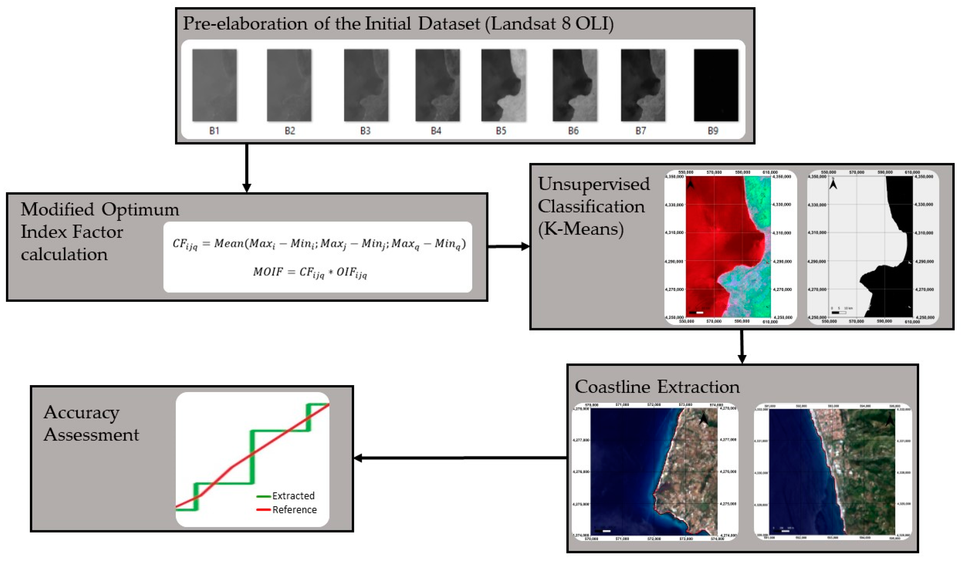
The workflow in Figure 2 shows the activies involved in the proposed method and the order they should go in. All steps can be developed in the GIS environment and the whole process may be automated using software tools that establish when one step has been completed successfully and the next step can begin.
Starting from the initial dataset (that includes all bands of Landsat 8 OLI), there is a pre-processing procedure for converting pixel values to reflectance. Subsequently, the MOIF values are calculated to establish the three bands to be subjected to the k-means for automatic classification. Finally, the coastline is extracted, and the accuracy of the results is evaluated. All these activities are described in detail in the following subsections.

3.1. Landsat Data OLI Pre-Elaboration

We used the formulas published by the USGS for converting the quantized and calibrated scaled digital numbers (DN) representing multispectral image data acquired by Landsat 8 OLI to top of atmosphere (ToA) reflectance [56].
Landsat data were converted from DNs to reflectance using the following formula:
ρ λ = M ρ   Q c a l + A ρ
where:
ρλ′ = TOA planetary reflectance, without correction for solar angle (note that ρλ’ does not contain a correction for sun angle);
= Band-specific multiplicative rescaling factor from the metadata (REFLECTANCE MULT BAND x, where x is the band number);
Qcal = Quantized and calibrated standard product pixel values (DNs);
= Band-specific additive rescaling factor from the metadata (REFLECTANCE ADD BAND x, where x is the band number).
Then, TOA reflectance with a correction for the sun angle is calculated using the formula:
R λ = ρ λ sin θ S E
where:
Rλ = TOA planetary reflectance;
θSE = Local sun elevation angle; the scene center sun elevation angle in degrees is provide in the metadata (SUN_ELEVATION).
Both formulas are applied using Raster Calculator, the QGIS tool that allows performance of multiple tasks of map algebra [57], i.e., mathematical calculations based on operators and functions, selection queries, or development in map algebra syntax [58].

3.2. Optimum Index Factor

The optimum index factor (OIF) was developed by Chavez et al. (1982) [46] as a method for determining the three-band combination that maximizes the variability in a particular multispectral scene [59]. The determination of the optimal combination of spectral intervals providing the maximum information with the minimum number of bands is of fundamental importance in remote sensing applications [60]. The OIF aims to maximize information content and avoid duplication. For this reason, it is based on the amount of total variance and correlation within and between all possible three-band combinations in the dataset [61]. OIF is calculated using the following formula:
O I F = S t d i + S t d j + S t d q | C o r r i , j | + | C o r r i , q | + | C o r r j , q |
where:
Stdi = standard deviation of band I;
Stdj = standard deviation of band j;
Stdq = standard deviation of band q;
Corrij = correlation coefficient of band i and band j;
Corriq = correlation coefficient of band i and band q;
Corrjq = correlation coefficient of band j and band q.
The larger the OIF value, the better the band combination.
Since the beginning OIF has been largely applied to Landsat datasets that include six multispectral bands with spatial resolution equal to 30 m (Landsat 5 and Landsat 7) or eight multispectral bands with the same spatial resolution (Landsat 8 and Landsat 9), so the selection of the most useful combination is crucial. Considering that they are also free of charge, we decide to use Landsat 8 OLI images for this study.
In our experiments, OIF was applied to each three-band combination, so 56 values were obtained, considering the 8 bands of Table 1.

3.3. Modified Optimum Index Factor

However, the OIF method has its limitations and there is no guarantee that the selected band subset is the optimal combination [62]. In fact, this index uses the correlation coefficient to identify the possibility of duplication of information and entrusts the variance with the task of identifying the amount of information. Bands with lots of “information” (high standard deviation) and a little “duplication” (low correlation between bands) will produce high OIF values [63]. However, the standard deviation may not be sufficient to underline the usefulness of an image in differentiating land cover classes. More useful for the purpose of identifying the amount of information present in an image would be the integration of the variance with the extension of the range of reflectance values present in the image itself. Even if they measure both the spread or variability of a dataset, variance and range are not coincident. In fact, two images with the same (low) variance value can present different widths of the reflectance range: the widest range carries out more information as it helps to better distinguish different types of land cover.
For example, Landsat 8 imagery includes the cirrus band, which provides information on the presence of clouds in the observed scene, effectively expressing a strong non-correlation with the other bands but characterized by a small amount of information on the investigated area. In other words, combinations including cirrus usually present a low level of correlation but also offer a low amount of information that does not contribute to accurately distinguish different land covers. Nevertheless, the low value of correlation with the other bands contributes to the high value of OIF while band compositions including images with limited range of values (like B9) are not optimal.
In this work, we proposed to overcome this drawback by introducing the corrective factor (CF) supplied by the following formula:
C F i j q = M e a n ( M a x i M i n i ; M a x j M i n j ; M a x q M i n q )
where i,j,q are the considered bands, Maxi, Maxj, Maxq are the maximum value of the respectively i,j,q selected bands, Mini, Minj, Minq are the minimum value of those bands. The amount of information present in each combination of bands is determined by the width of the range of values of each band: the wider the ranges, the higher the CF value.
The product between CF and OIF determines the MOIF:
M O I F = C F i j q O I F i j q
In other terms, MOIF incorporates in a single value the degree of non-correlation and the amount of information in better way than OIF as it introduces a multiplication factor which is the average of the extensions of the reflectance ranges of the three bands considered. The higher the MOIF value, the stronger the contrast between water and non-water.
Similarly to OIF, MOIF produced 56 values in our study, one for each three-band combination.
Note that band selection is an effective pre-processing way to reduce the number of available images and use only those that are useful for a particular perspective [64]. Most of the existing methods select bands according to a single criterion, such as the extraction of specific features, e.g., roads, water body, forests, etc. Usually, it is necessary to set up different band combination schemes according to the spectral characteristics for different observation objects. In fact, if on the one hand the spectral signature allows recognition of an object or a type of land cover [65], on the other hand there are definite wavelength values that better enhance the specificity of the spectral response of this object or land cover, such as (630–690 nm), and (770–895 nm) for vegetation [66]. Consequently, there are some bands that are better than others in enhancing the difference of such objects or land covers [65]. The water indices, such as NDWI, automated water extraction index (AWEI) [67], modified normalized difference water index (MNDWI) [68], based on the selection of two or more bands that better highlight the behavior of water bodies with respect to the context, are also part of this perspective. However, the bands that allow water to be highlighted in a scene, including bare soil and vegetation, are usually uncorrelated and with a wide range of different values, as is the case for NIR and/or SWIR bands compared to the visible. We believe that looking for uncorrelated bands with a high information content can lead to precise selection of those same bands that are involved in the water indices or help define new indices.

3.4. Image Classification Using K-Means

Clustering is a process that divides a set of objects into groups (clusters) according to the predefined criteria such that objects in the same cluster are more similar to each other than other objects in different groups [69]. K-means clustering is a popular technique in analysis and pattern recognition [70]. It is an unsupervised classification algorithm, in particular belonging to family of partitional clustering that decomposes a dataset into a set of disjoint groups [71].
The k-means algorithm was proposed by J. MacQueen [72] and the main purpose is to describe a process for partitioning an N-dimensional population in k sets on the basis of a sample. In other words, the goal is to produce groups of variables with a high degree of similarity within each group and a low degree of similarity between groups [73]. In the k-means algorithm, the choice of number of k classes or clusters for classification which is established a priori is important. For every cluster, the position of centroids in the dataset is defined, which represents the center of the cluster. K-means is an iterative algorithm that performs the procedure of iteration until the centroids’ position is stabilized. The k-means algorithm consists in the following steps:
  • Define k cluster and select k centroids from dataset randomly as initial clustering center;
  • Calculate the Euclidean distance between k initial centroids and the data points of dataset and assign each data point to cluster with minimum distance;
  • Calculate the average of data points that belongs to each cluster and reposition the new centroids;
  • Repeat the second and third step until the centroids are not changing, which means the convergence point is reached, in order to obtain unchangeable cluster.
K-means is applied to the whole dataset as well as to all three-band compositions. The binary maps produced by applying the k-means were submitted to automatic vectorization, finally producing 57 different coastlines, one for the whole dataset, the others resulting from three-band compositions.

3.5. Accuracy Tests

Accuracy tests were carried out on a selected subset of the resulting coastlines. In the literature, quantitative assessments are usually conducted by comparing the detected coastlines with the reference one, which is manually delineated coastline [17,74]. In this study, we compared each selected coastline with the reference one, achieved by photointerpretation and manual vectorization on the RGB true color composition. Particularly, we considered the coastline resulting from the unsupervised classification of all bands as well as those derived from 14 of the 56 three-band compositions. This selection aimed to analyze the accuracy of the results related to the variability of MOIF, so subsets presenting high, middle and low values of the proposed new index were chosen. In addition, we also selected two band combinations presenting the higher values of OIF (i.e., the first and the second classified) to better compare the different results provided by the two indices considered.
Due to the imperfect overlap between each automatic extracted coastline and the reference coastline, polygons were generated by the layer overlay. In the literature, there is a methodology that allows deriving the level of accuracy of the shift between these two lines, called the distributed ratio index (DRI) [34]. This derives from the ratio index (RI) which is given by the ratio between the sum of the areas of the polygons (A) and the length of the coastline chosen as a reference (L):
R I = A L
The difference between these two indices is that the DRI also provides parameters such as the standard deviation, and the minimum and maximum values of the shift, in order to supply the degree of accuracy. In fact, this index considers the area of each polygon generated (Ak), dividing it with the length of effective coastline (Lk) on which it develops. In this way, the values express more detailed information on the residuals and furthermore it is possible to provide the statistical parameters. The formula is:
D R I = A k L k
where Ak is the area of the k-th element, Lk is the length of the coastline of the k-th stretch. In consequence, DRI supplies n values, one for each polygon generated between the reference coastline and the extracted coastline.
In addition, to verify the thematic accuracy of the unsupervised classification, obtained for each considered band composition, test sites are used. The manual vectorization of the coastline divides the scene into two macro areas, i.e., sea and land. Since the classification difficulty is mainly for the pixels near the coastline, we decided to consider a buffer of 300 m around the land–sea separation line. In this way, there were two extensive test sites, one of water and the other of no-water separated by the coastline.
In this way, it was possible to determine each time how many pixels were correctly and incorrectly classified. In particular, we proceeded with the construction of the confusion matrix: it is a powerful tool that determines and quantifies the correctness of the classification. The confusion matrix is nothing more than a table of values where each row represents the real values, while each column the predicted values. In the diagonal there are the elements classified correctly, i.e., belonging to the “true” class. From this matrix, it is possible to calculate three significant accuracy values, called user accuracy (UA), producer accuracy (PA) and overall accuracy (OA).
The UA is given by the number of accurately classified pixels divided by the pixels assumed as belonging to that class. PA is the ratio of correctly classified pixels to the total pixels belonging to that class. Finally, OA is given by the total of correctly classified pixels of each class divided by the total pixels [75].

4. Results and Discussion

4.1. OIF and MOIF Results

The resulting OIF values for the 56 band combinations are listed in Table 2 in descending order (the higher the value, the better the ranking).
In the first positions of the ranking provided by the OIF index, there are the band compositions including B9, as was to be expected. In fact, as mentioned in the previous section, the cirrus band has characteristics that make it strongly decorrelated from the others. It generally has brighter pixels for presence of clouds and dark ones in other areas: the main feature is the visualization of clouds at high altitude, which could not be visible in other spectral bands. Although B9 has poor information on the land cover of the investigated scene, our experiments confirmed that in many cases, band compositions including cirrus presented high values for OIF. Due to this problem, a new ranking was drawn up given by the new index (MOIF).
The maximum, minimum and difference values of the bands that are necessary for calculating CF (Equation (4)) are reported below (Table 3).
The maximum and minimum values provide further confirmation of the poor information of B9, when compared to the other bands. The difference obtained between the maximum and the minimum of each band allowed us to calculate the MOIF index that substantially changed the ranking of the band combinations (Table 4).
The new ranking obtained overturns the previous one. We can see that the first classified compositions do not have the cirrus band: since the aim is to identify optimal subsets that ensure a lot of information to better distinguish the types of land cover, the classification is more reliable.

4.2. K-Means Application

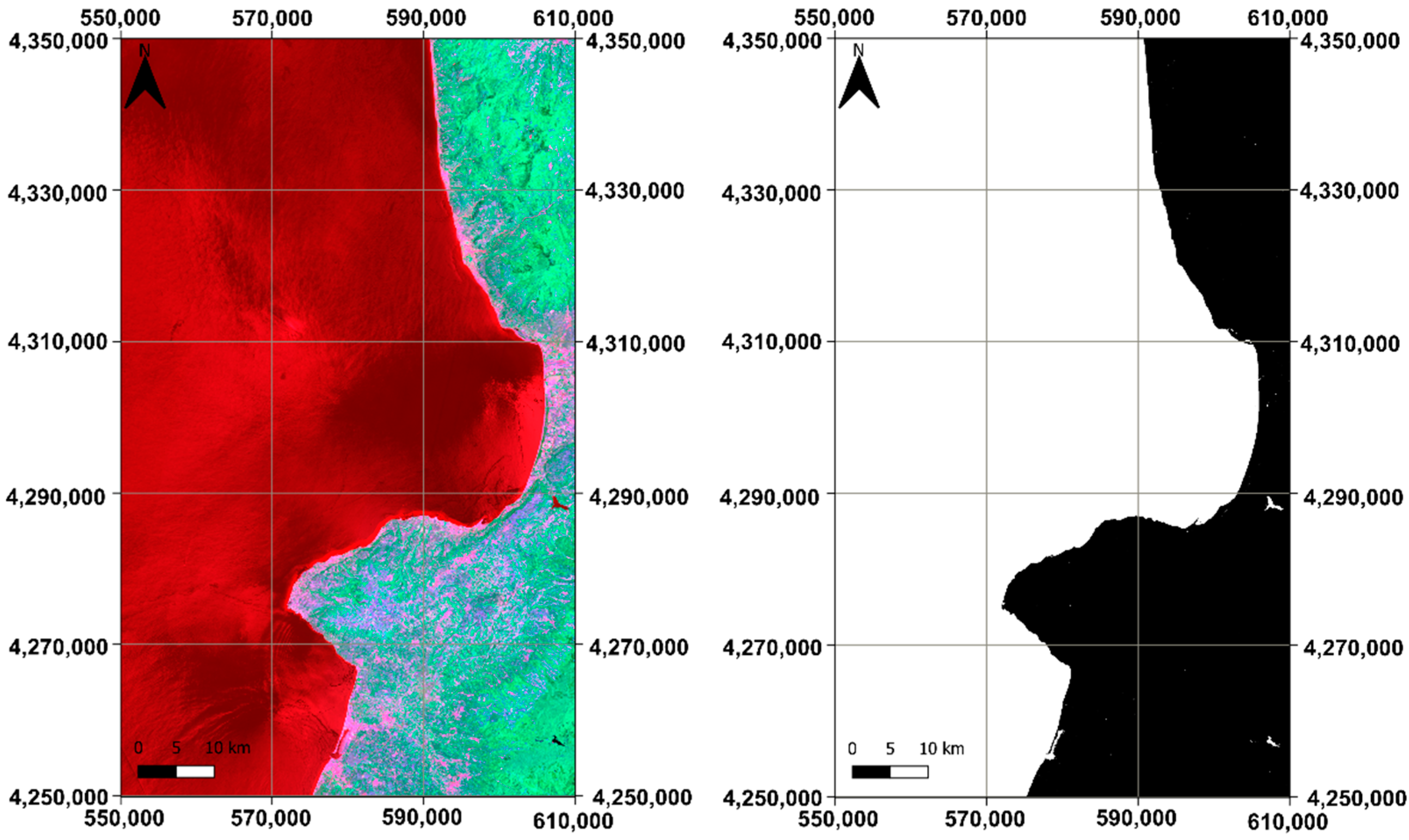
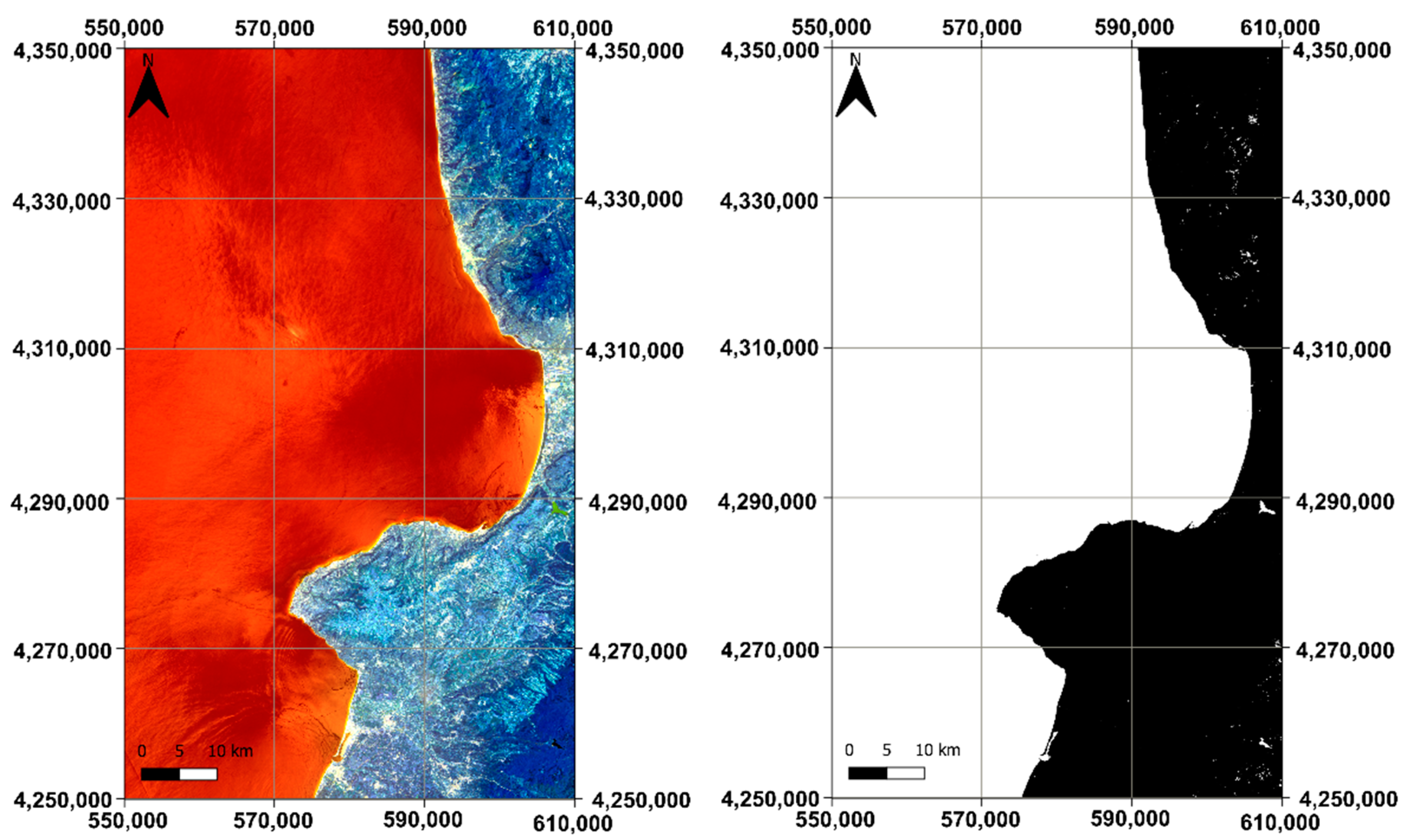
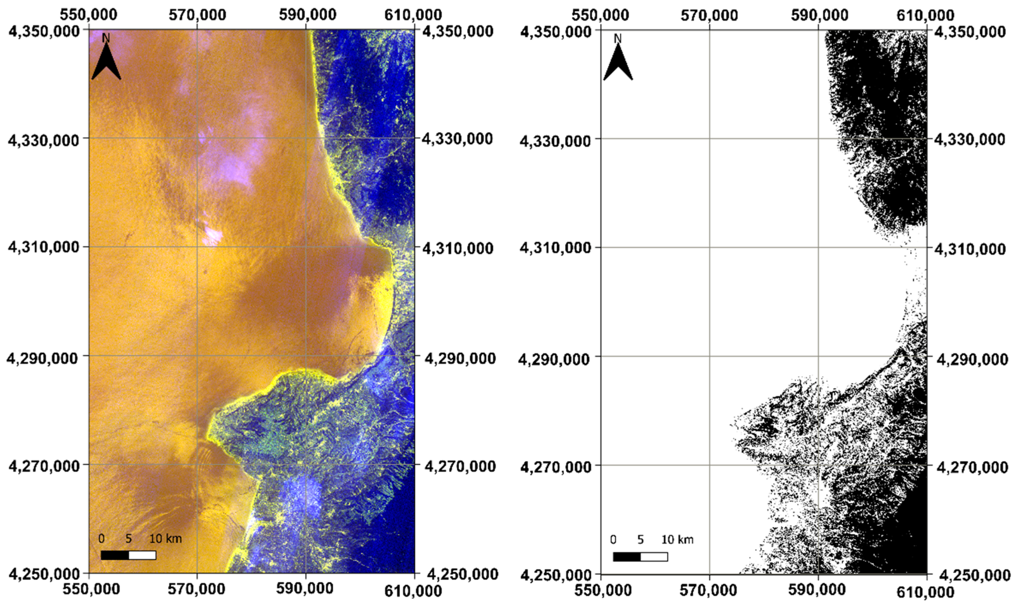
In this section, three emblematic false color compositions and their k-means classification are shown. Particularly, the first (Figure 3), the middle (Figure 4) and the last classified (Figure 5) based on MOIF values are selected.
From a first visual analysis, as the MOIF decreases, the classification worsens, and therefore the separation between sea and land given by the coastline is less accurate. In particular, the k-means application to the composition of the bands 1-2-9 returned a great part of Calabria territory fragmented as many islands surrounded by the sea that penetrates for many kilometers inside the land. The result was clearly wrong and there was no need to calculate DRI for certifying the unreliability of the coastline extractable in this case. Nonetheless, in order to have a numerical type of analytical indicator that allowed ranking the compositions of bands in relation to the accuracy of the coastline that can be extracted from them, DRI was calculated in each of the possible cases.

4.3. DRI Evaluation

Table 5 shows the statistics of DRI obtained for 15 of the resulting coastlines. Particularly, we considered the coastline supplied by the k-means application to the following band compositions:
  • The group including all Landsat OLI multispectral bands (B1, B2, B3, B4, B5, B6, B7, B9);
  • The first three classified band composition given by MOIF (B2, B5, B6; B2, B5, B7; B5, B6, B7);
  • Three classified respectively 12th, 21st and 26th given by the MOIF (B3 B5 B6; B2 B3 B5; B3 B4 B5);
  • The two middle classified band composition given by MOIF (B2, B3 B6; B1 B3 B6);
  • One classified 43rd given by the MOIF (B3 B4 B6)
  • The last three classified given by MOIF (B2, B3, B9; B3, B4, B9; B1, B2, B9);
  • The first two classified band composition given by OIF (B2, B5, B9; B4, B5, B9).
For comparison with the pixel size, i.e., 30 m, as well as to establish the accuracy of the extracted coastline, the DRI results are given in meters.
The DRI values show a better performance as the MOIF index increases. The first classified composition, including blue, NIR and SWIR1 bands (B2 B5 B6), has the best RMSE value (9.108 m), while the maximum (35.940 m) is close to pixel dimension. The two band compositions following in the standings show slightly worse results (RMSE equal to 9.242 m and 9.243 m, respectively).
The composition of the band classified 12th has a very excellent RMSE value (9.281 m) if compared to the first three, worsening the maximum value (81.696 m). The other two band compositions taken into consideration (21st and 26th) stabilize their RMSE value around the value 9.4 m as well as the maximum shift reached (about 82 m).
Instead, for the 28th and 29th classified compositions we can see RMSE values (respectively 9.637 m and 9.692 m) that still do not differ much from that of the first classified composition, but the maximum value so far remains more than double the pixel size (83.120 m).
Starting from the 43th composition, a deterioration is noted both in terms of RMSE (14.537 m) and maximum (623.013 m).
The 54th composition according to MOIF values shows that the high correlation between B2 and B3 as well as the low level of information included in B9 aggravates the accuracy of the extracted coastline. In fact, in this case, we have bad statistics for DRI (RMSE equal to 72.022 m and maximum equal to 952.779 m). The situation is becoming worse for the last classified band compositions (B3, B4, B9 and B1, B2, B9), showing a rapid increase of the shift between each extracted coastline and the reference one.
In addition, the last two combinations of bands (B2, B5, B9 and B4, B5, B9) slip from the top positions, given by the OIF, to the 18th position and 13th position, respectively, according to the MOIF index. The results show that the application of the new index is consistent with the variation in the results supplied by the accuracy evaluation.
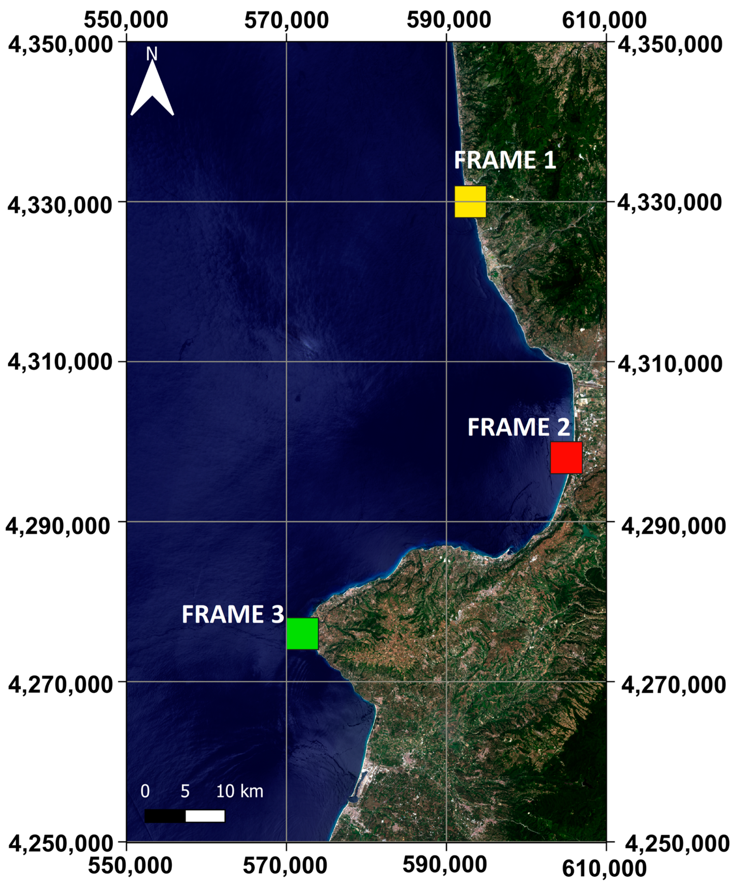
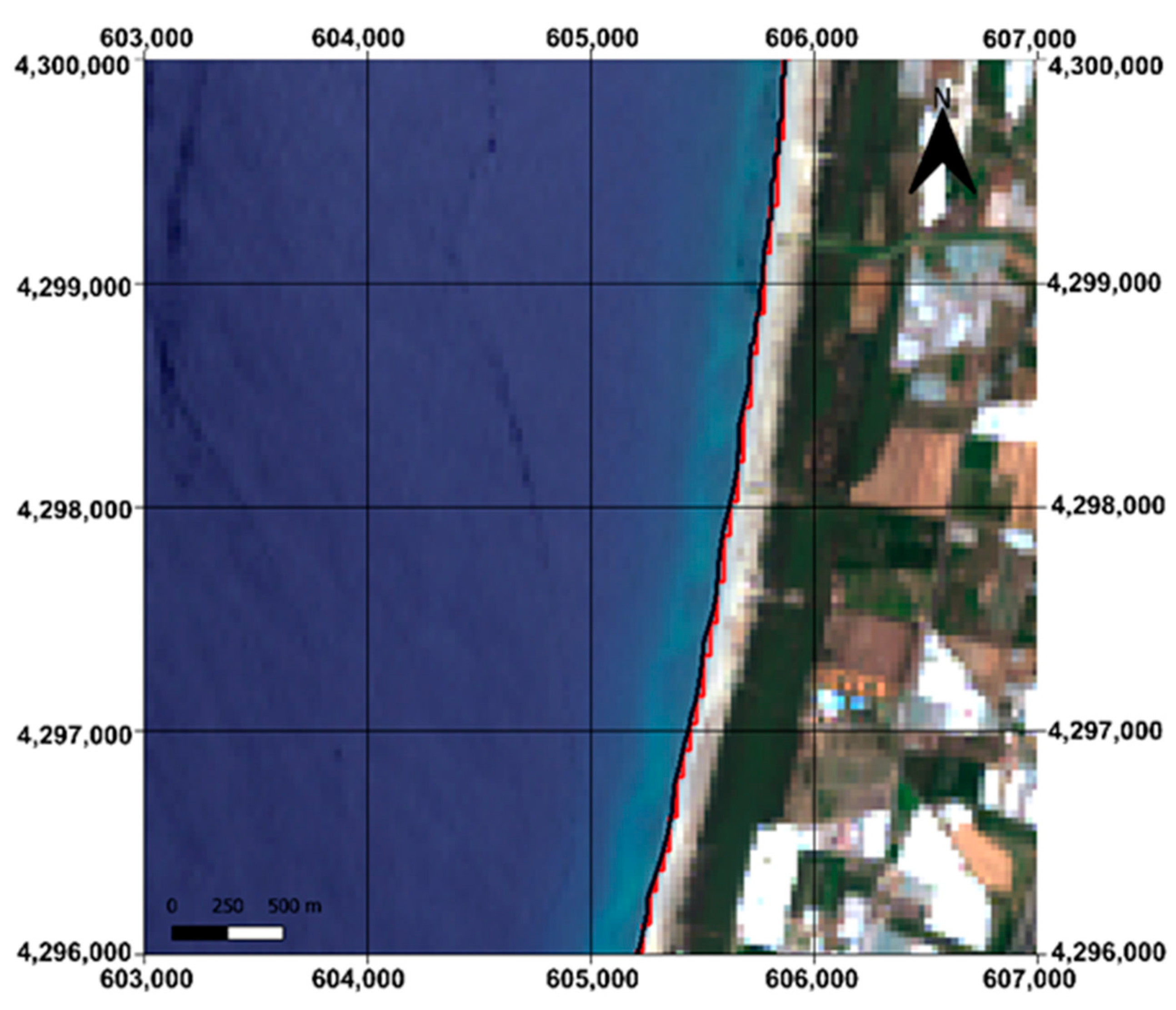
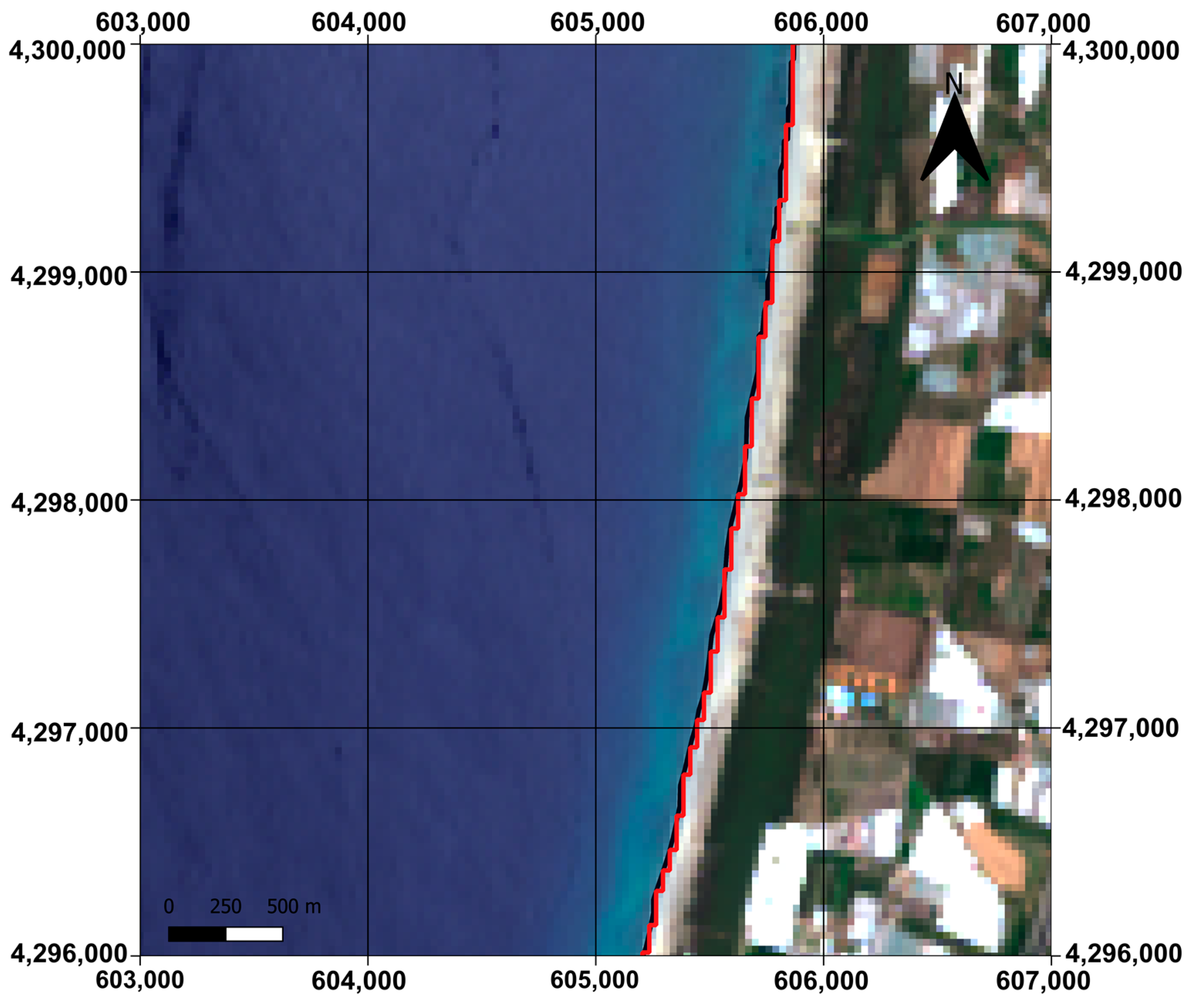
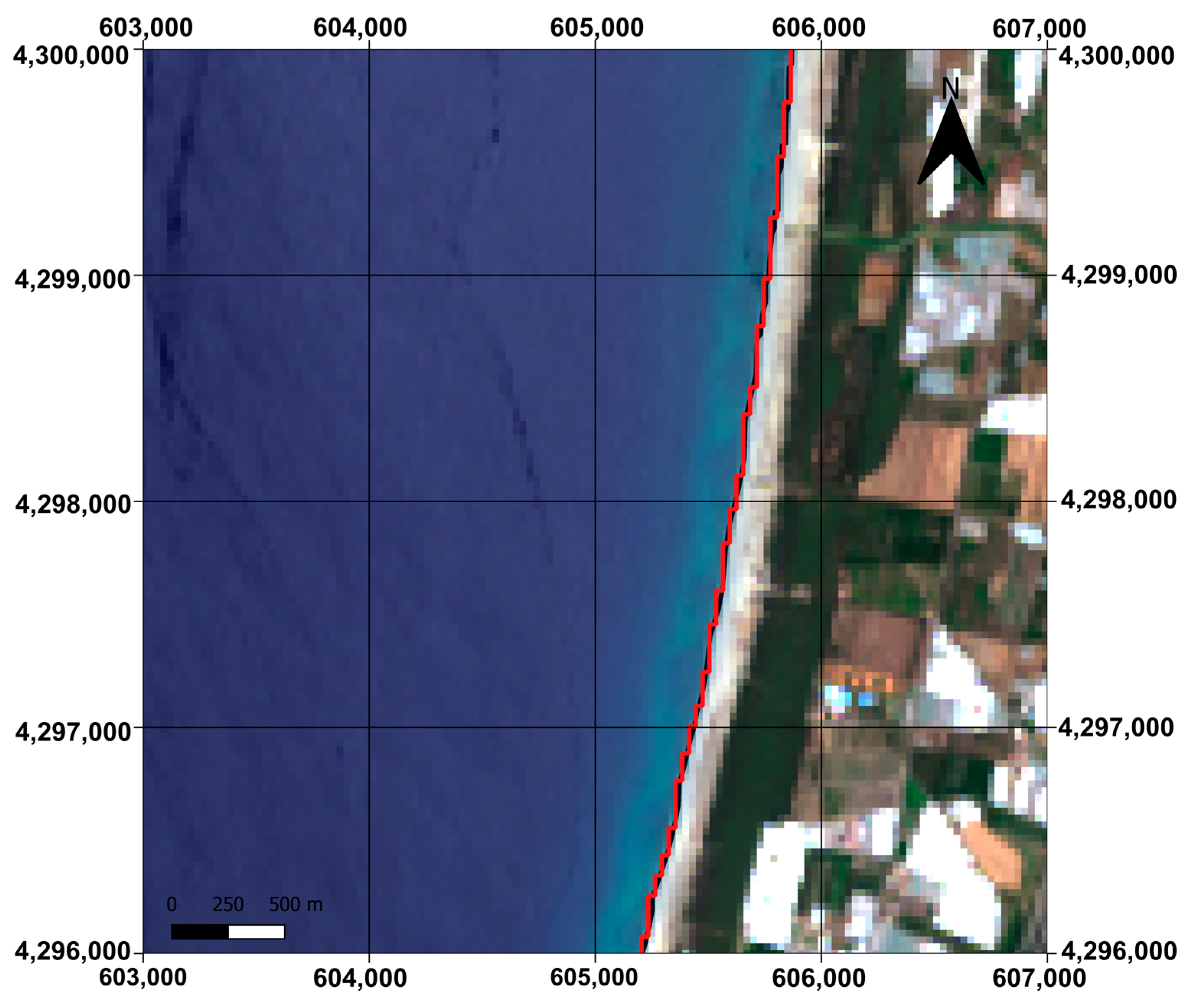
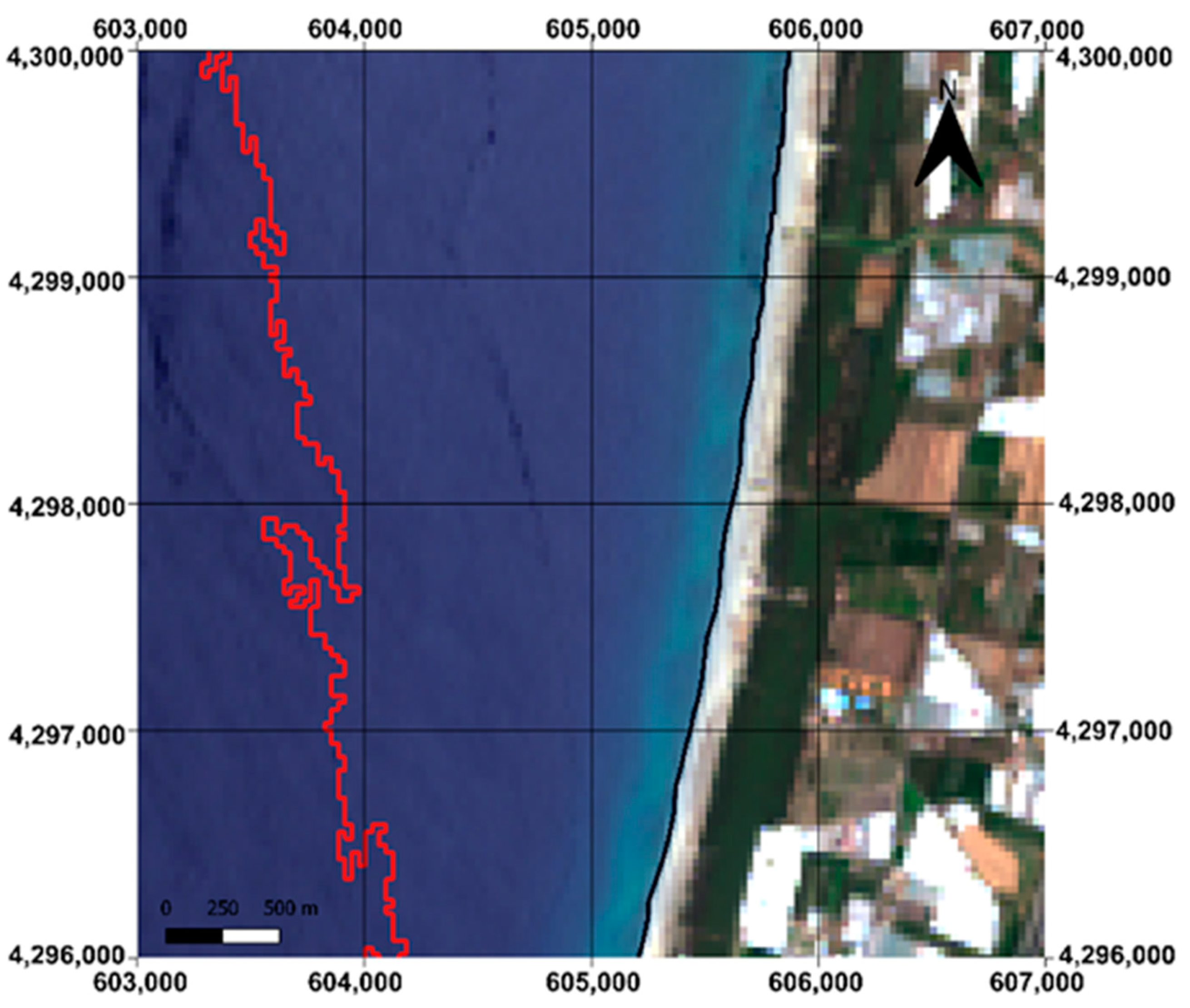
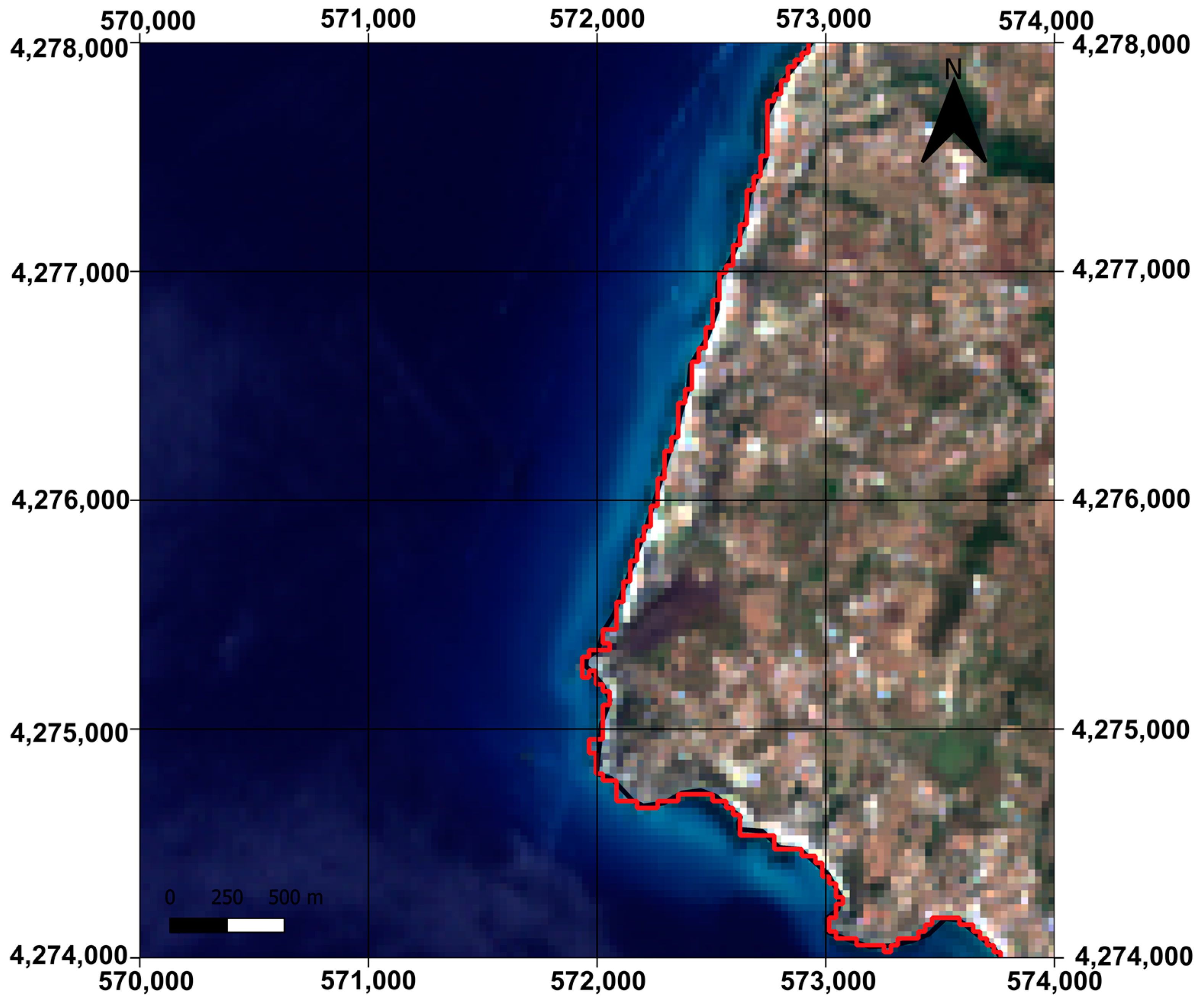
To show on map the different accuracy level of results related to the MOIF values, we selected three zones respectively in the north (Frame 1), middle (Frame 2) and south part (Frame 3) of the study area (Figure 6).
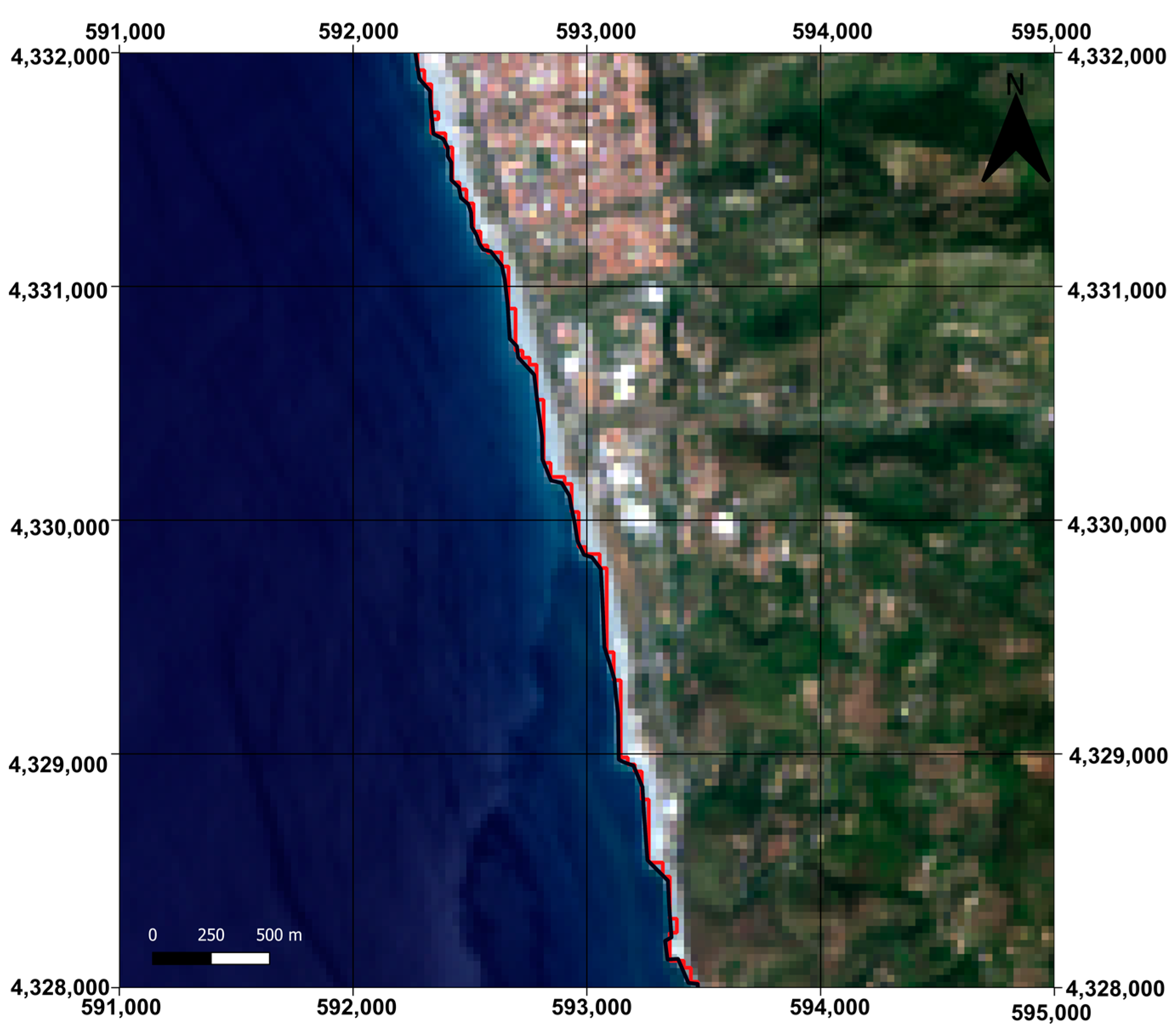
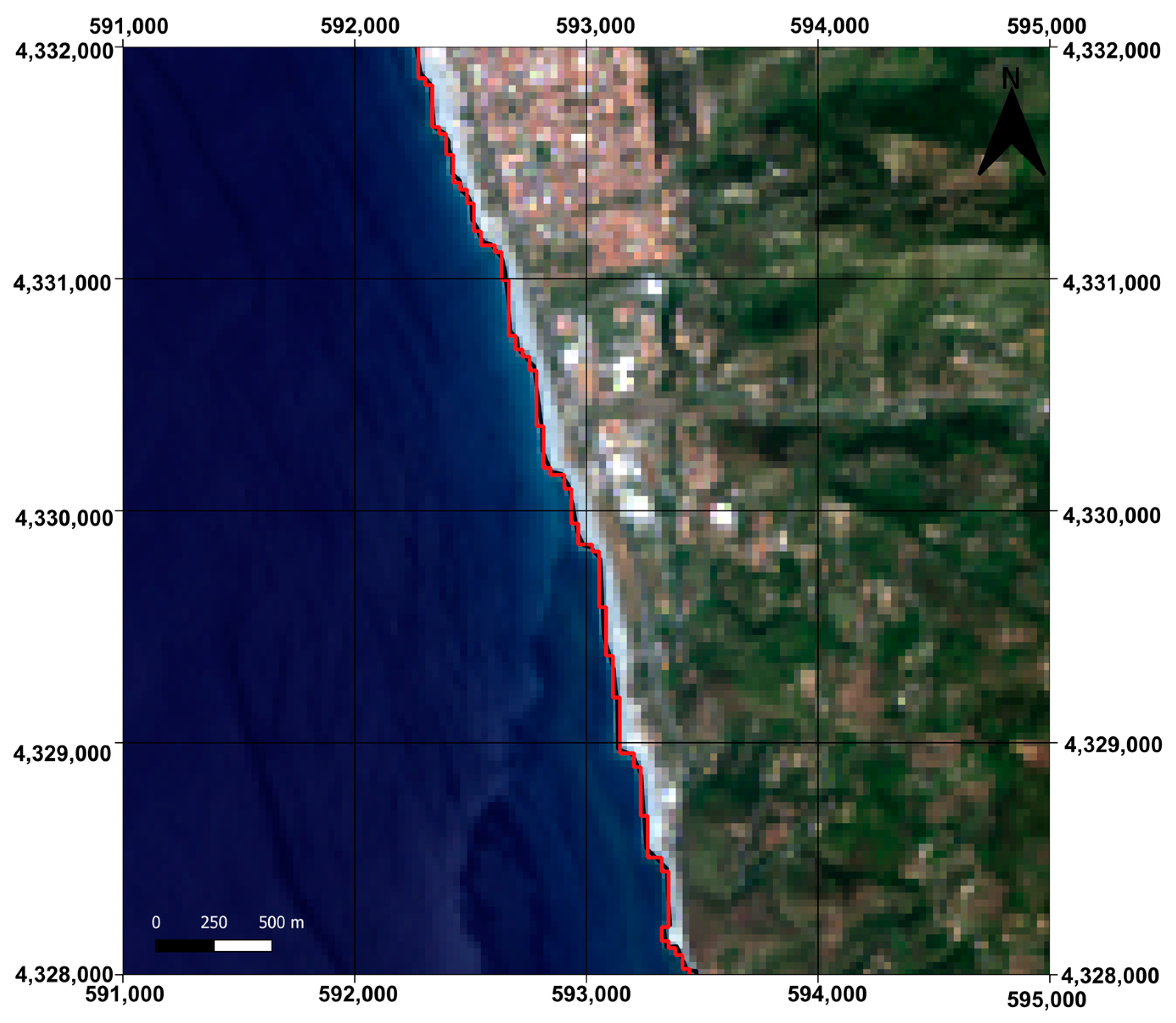
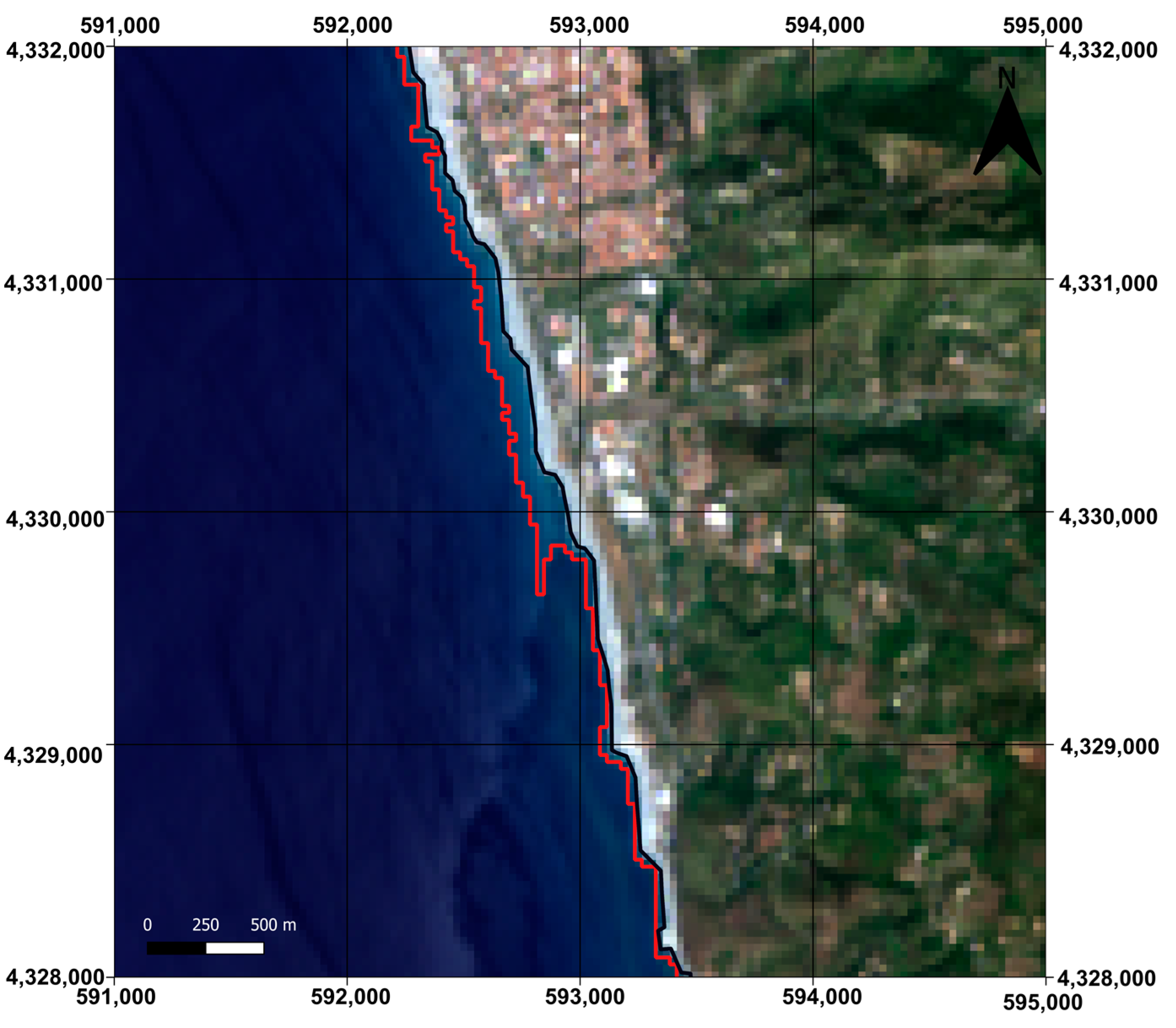
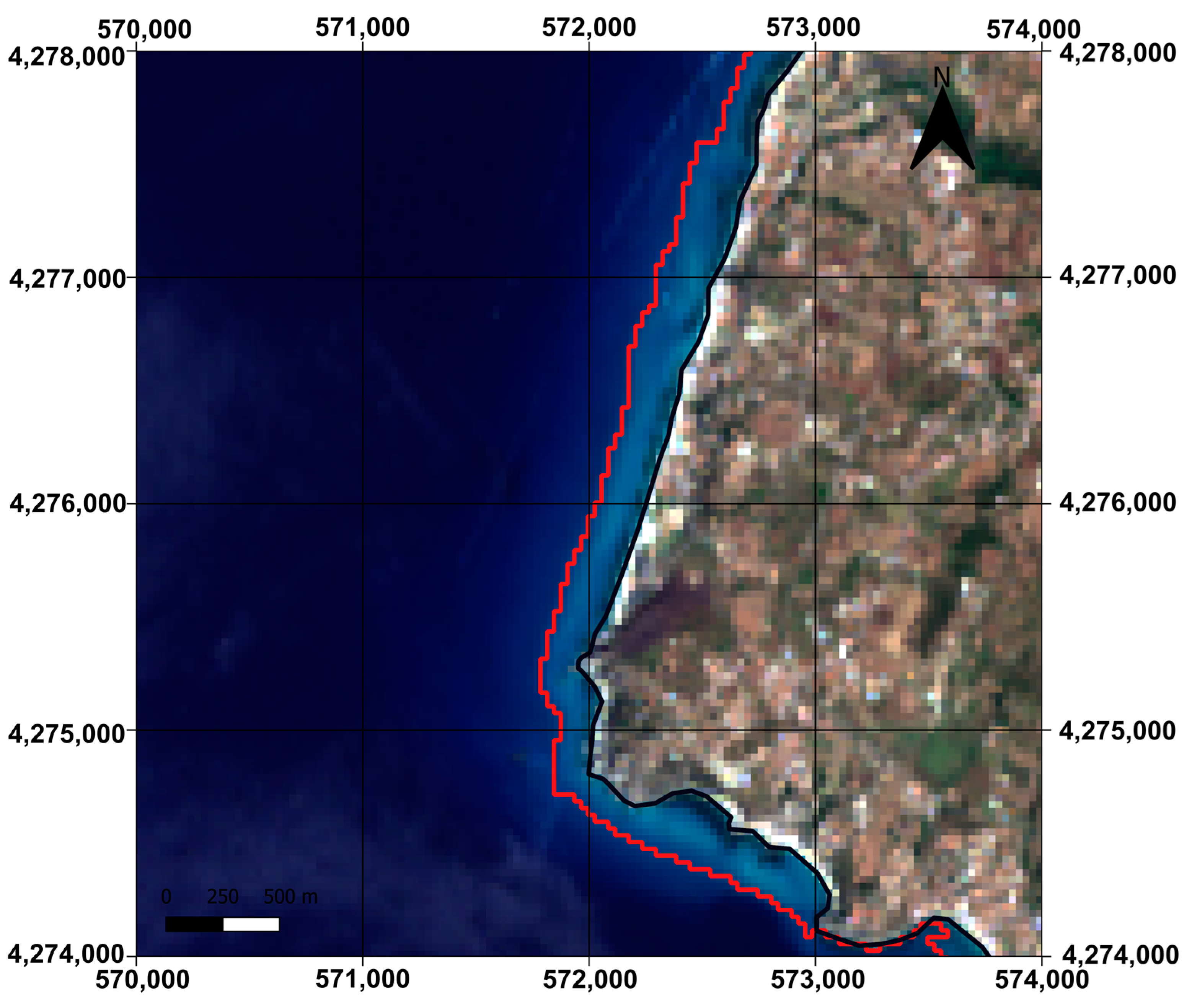
Four scenarios were considered for each frame, the first associated with the best performing band composition (B2, B5, B6), the second associated with a composition classified at the 24th position (B3, B4, B5), the third associated with a composition classified at the 43th position (B3, B4, B6), and the fourth presenting one of the worst performances associated with a composition classified at the 54th position (B2, B3, B9), as resulting from the DRI application. The results of the above mentioned band compositions for the frame 1 are shown in the Figure 7(B2, B5, B6), Figure 8(B3, B4, B5), Figure 9(B3, B4, B6) and Figure 10(B2, B3, B9). In analogous way, Figure 11, Figure 12, Figure 13 and Figure 14 concern the frame 2 and Figure 15, Figure 16, Figure 17 and Figure 18 the frame 3, repeating the band compositions in the same order.
In each case, the automatically extracted coastline (in red) was compared to the reference coastline (in black).
Due to the raster to vector conversion, the lines are jagged, as they followed the shape of the pixel (smoothing was not applied in our experiments). In all cases, the coastline extracted from the band composition associated to the higher value of MOIF was very close to the reference coastline. Vice versa, maps showed very high deviations between the reference coastline and the coastline extracted from the band composition associated to a low value of MOIF.
The images above highlight the effectiveness of the index used, emphasizing how the decorrelation among the bands and the amount of information in each band influenced the accuracy of the automatic extracted coastline. In fact, as the value of the MOIF decreases, we see a gradually increasing distance between the reference coastline and the one automatically extracted from the considered band combination.

4.4. Classification Accuracy Evaluation

Table 6 shows the thematic accuracy values for the 15 band compositions selected for our tests and classified with the k-means.
The OA accuracy values close to 1 indicate correct classification.
The results of the thematic accuracy are also very satisfactory and in fact confirm in other terms what the DRI had already anticipated. The first band combination, given by the MOIF, (B2, B5, B6), also remains the best in this case reaching the highest OA value, as well as proceeding from the highest to the lowest MOIF value, the OA decreases, synonymous with a worsening classification. In fact, in the last places we find the band compositions(B3, B4, B9 and B1, B2, B9) that have a low OA value (0.8).

4.5. Comparison with Other Study Results

Finally, we can evaluate the effectiveness of the proposed approach comparing the results with those obtained by other researchers, especially in terms of accuracies achievable using different methods.
Liu et al. [25] in 2017 analyzed the performance of coastline extraction by integrating downscaling, pan-sharpening and water index approaches in increasing the accuracy of coastline extraction from Landsat 8 OLI images. They considered a portion of Ningbo coast (East China Sea) mainly containing bedrock coast, artificial coast and flat sandy coast and used ZiYuan-3 surveying satellite (ZY-3) MS image to extract the reference coastline. Applying the traditional water index method to extract coastline directly from original MS images (resolution: 30 m), they obtained a mean absolute difference (MAD) equal to 18.62 m between the resulting coastline and the reference one, with maximum positive difference (MPD) equal to 124.19 m and minimum negative difference (MND) equal to 223,89 m. Better results were achieved using pan-sharpened images (MAD = 13.54 m, MPD = 129.47, MND = 107.11 m) but those are not comparable with our study, which does not consider data fusion. However, the approach we propose based on MOIF and K-means ensures better accuracies and not only with the first classified band combination (B2, B5, B6), but also with others, such as B2, B5,B7; B5,B6, B7; B3, B5, B6; B2, B3, B5 and B3, B4, B5.
In 2017, El Kafrawy et al. [76] examined the performance of six different methods used to extract shorelines from Landsat 8 images. They compared the output with a shoreline detected by high-resolution image Pleiades B1 (0.50 m). The experiments showed that all coastlines extracted were within a pixel shift (30 m), but the thresholding band ratio method was the most accurate approach with an RMSE of 9.54 m, which is still less accurate than results we obtained with our approach.
Tuan et al. in 2018 [77] evaluated the accuracy of coastline extraction using three water indices (NDWI, MNDWI and AWEI) applied to Landsat 8 imagery and compared the results with a practical shoreline, obtained considering ground-truthing positions identified during a field survey. This study revealed that the AWEI was a more accurate approach than NDWI and MNDWI, with an RMSE of 12.4 m.
Alcaras et al. [78] in 2019 applied NDWI to Landsat 8 OLI images to detect the Tyrrhenian coastline of the Campania region (Italy) presenting, similarly with our study area, long beaches as well as high coasts and port zones [79]. Alcaras et al. used maximum likelihood classification (MLC), one of the most common classification methods in remote sensing based on Bayes’ theorem, to determine a threshold to separate seawater from land in an NDWI map. They obtained MAD=16.84 m between the resulting coastline and the reference one, achieved with visual interpretation and manual vectorization of RGB composition. In this case, the accuracy was also lower than that provided by the method we propose.

5. Conclusions

The experiments carried out on Landsat 8 OLI images concerning a part of the Calabria region highlight the effectiveness of the proposed approach for coastline data automatic extraction based on an unsupervised method, such as the k-means, and the use of a new index, the MOIF. This index gives as a single value the combination of the degree of correlation and the amount of information overall provided by the specific three bands considered. In other words, this index makes it possible to identify the three bands which simultaneously are highly uncorrelated and exhibit a wide range of values, so as to facilitate the distinction between water and no-water (i.e., soil and vegetation).
To establish the accuracy of the results, we used the DRI, which provided the deviation between the reference coastline and the automatically extracted one, as well as thematic accuracy indices (i.e., PA, UA and OA) extracted from confusion matrix. Both approaches corroborated the validity of the proposed method. In fact, the results were very encouraging: the best three-band composition given by the new index, i.e., B2, B5, B6, provided the best statistics of DRI, with RMSE value lower than the pixel dimensions and with a maximum value slightly exceeding this dimension. DRI confirmed that the effectiveness of MOIF seems to be better than that of OIF in selecting the optimal three-band composition for coastline extraction. Similarly, the thematic accuracy provided by the OA values confirmed the indications of the MOIF: the best resulting combination was B2, B5, B6.
The experiments carried out show that it is preferable to apply k-means on a three-band composition rather than on all available bands at the same time: DRI values and thematic accuracy indices confirm that increasing the data to be processed in the unsupervised classification can introduce confusion, as in this case, and worsen the results rather than produce an enhancement of the thematic accuracy.
Regarding the future developments of this work, further studies will be focused on the possibility of extending the proposed approach to other satellite images, especially those presenting higher resolution than Landsat 8 OLI, in order to evaluate the correctness of the suggested index, i.e., MOIF, for the identification of the three uncorrelated bands including a high level of information. Furthermore, we will mainly focus on the possibility to find the best method for automatic coastline data extraction comparing the proposed approach with others available in literature such as water index approaches (e.g., NDWI) and machine learning approaches.

Author Contributions

C.P. conceived the article and designed the experiments; F.G.F. and A.V. conducted the bibliographic research; F.G. organized the data collection; C.P. supervised the applications; F.G.F. carried out experiments on OIF applications; C.P. designed the MOIF; F.G. carried out experiments on MOIF; A.V. carried out the accuracy tests; all authors took part in the result analysis and in writing the paper. All authors have read and agreed to the published version of the manuscript.

Funding

This research received no external funding.

Data Availability Statement

The study’s data are available upon request from the corresponding author for academic research and non-commercial purposes only. Restrictions apply to derivative images and models trained using the data, and proper referencing is required.

Conflicts of Interest

The authors declare no conflict of interest.

References

  1. National Geographic, Coast. Available online: https://education.nationalgeographic.org/resource/coast/ (accessed on 14 April 2023).
  2. Maglione, P.; Parente, C.; Vallario, A. Coastline Extraction Using High Resolution WorldView-2 Satellite Imagery. Eur. J. Remote Sens. 2014, 47, 685–699. [Google Scholar] [CrossRef]
  3. Pepe, M.; Parente, C. Burned Area Recognition By Change Detection Analysis Using Images Derived From Sentinel-2 Satellite: The Case Study Of Sorrento Peninsula, Italy. J. Appl. Eng. Sci. 2018, 16, 225–232. [Google Scholar] [CrossRef]
  4. Seale, C.; Redfern, T.; Chatfield, P.; Luo, C.; Dempsey, K. Coastline Detection in Satellite Imagery: A Deep Learning Approach on New Benchmark Data. Remote Sens. Environ. 2022, 278, 113044. [Google Scholar] [CrossRef]
  5. Di, K.; Wang, J.; Ma, R.; Li, R. Automatic Shoreline Extraction from High Resolution IKONOS Satellite Imagery. In Proceedings of the ASPRS 2003 Annual Conference, Anchorage, Alaska, 5–9 May 2003. [Google Scholar]
  6. Duarte Viana, R.; Nicola Lima dos Reis, G.; Maria Gomes Velame, V.; Sehn Körting, T. Shoreline Extraction Using Unsupervised Classification On Sentinel-2 Imagery. In Proceedings of the 2019 Galoá Proceedings of XIX Brazilian Symposium on Remote Sensing, Santos, SP, Brazil, 14–17 April 2019; pp. 2422–2425. [Google Scholar]
  7. Toure, S.; Diop, O.; Kpalma, K.; Maiga, A.S. Shoreline Detection Using Optical Remote Sensing: A Review. ISPRS Int. J. Geo-Inf. 2019, 8, 75. [Google Scholar] [CrossRef] [Green Version]
  8. Dellepiane, S.; De Laurentiis, R.; Giordano, F. Coastline extraction from SAR images and a method for the evaluation of the coastline precision. Pattern Recognit. Lett. 2004, 25, 1461–1470. [Google Scholar] [CrossRef]
  9. Yu, S.; Mou, Y.; Xu, D.; You, X.; Zhou, L.; Zeng, W. A New Algorithm for Shoreline Extraction from Satellite Imagery with Non-Separable Wavelet and Level Set Method. IJMLC 2013, 3, 158–163. [Google Scholar] [CrossRef] [Green Version]
  10. Qiu, S.; Ye, H.; Liao, X. Coastline Recognition Algorithm Based on Multi-Feature Network Fusion of Multi-Spectral Remote Sensing Images. Remote Sens. 2022, 14, 5931. [Google Scholar] [CrossRef]
  11. Liu, H.; Jezek, K.C. Automated Extraction of Coastline from Satellite Imagery by Integrating Canny Edge Detection and Locally Adaptive Thresholding Methods. Int. J. Remote Sens. 2010, 25, 937–958. [Google Scholar] [CrossRef]
  12. Baud, I.; Kuffer, M.; Pfeffer, K.; Sliuzas, R.; Karuppannan, S. Understanding Heterogeneity in Metropolitan India: The Added Value of Remote Sensing Data for Analyzing Sub-Standard Residential Areas. Int. J. Appl. Earth Obs. Geoinf. 2010, 12, 359–374. [Google Scholar] [CrossRef]
  13. Forestier, G.; Wemmert, C.; Puissant, A. Coastal Image Interpretation Using Background Knowledge and Semantics. Comput. Geosci. 2013, 54, 88–96. [Google Scholar] [CrossRef] [Green Version]
  14. Kuenzer, C.; Ottinger, M.; Liu, G.; Sun, B.; Baumhauer, R.; Dech, S. Earth Observation-Based Coastal Zone Monitoring of the Yellow River Delta: Dynamics in China’s Second Largest Oil Producing Region over Four Decades. Appl. Geogr. 2014, 55, 92–107. [Google Scholar] [CrossRef]
  15. Alcaras, E.; Amoroso, P.P.; Baiocchi, V.; Falchi, U.; Parente, C. Unsupervised Classification Based Approach for Coastline Extraction from Sentinel-2 Imagery. In Proceedings of the 2021 International Workshop on Metrology for the Sea; Learning to Measure Sea Health Parameters (MetroSea), Reggio Calabria, Italy, 4–6 October 2021; pp. 423–427. [Google Scholar] [CrossRef]
  16. Nagendra, H.; Gadgil, M. Biodiversity Assessment at Multiple Scales: Linking Remotely Sensed Data with Field Information. Proc. Natl. Acad. Sci. USA 1999, 96, 9154–9158. [Google Scholar] [CrossRef] [PubMed] [Green Version]
  17. Maglione, P.; Parente, C.; Santamaria, R.; Vallario, A. Modelli Tematici 3D Della Copertura Del Suolo a Partire Da DTM e Immagini Telerilevate Ad Alta Risoluzione WorldView-2. Rend. Online Della Soc. Geol. Ital. 2014, 30, 33–40. [Google Scholar] [CrossRef]
  18. Alcaras, E.; Amoroso, P.P.; Figliomeni, F.G.; Parente, C.; Prezioso, G. Accuracy Evaluation of Coastline Extraction Methods In Remote Sensing: A Smart Procedure For Sentinel-2 Images. Int. Arch. Photogramm. Remote Sens. Spat. Inf. Sci. 2022. [Google Scholar] [CrossRef]
  19. Gao, Y.; Mas, J.F. A Comparison Of The Performance Of Pixel-Based And Object-Based Classifications Over Images with Various Spatial Resolutions. Online J. Earth Sci. 2008, 2, 27–35. [Google Scholar]
  20. Liu, D.; Xia, F. Assessing Object-Based Classification: Advantages and Limitations. Remote Sens. Lett. 2010, 1, 187–194. [Google Scholar] [CrossRef]
  21. Myint, S.W.; Gober, P.; Brazel, A.; Grossman-Clarke, S.; Weng, Q. Per-Pixel vs. Object-Based Classification of Urban Land Cover Extraction Using High Spatial Resolution Imagery. Remote Sens. Environ. 2011, 115, 1145–1161. [Google Scholar] [CrossRef]
  22. Zhang, T.; Yang, X.; Hu, S.; Su, F. Extraction of Coastline in Aquaculture Coast from Multispectral Remote Sensing Images: Object-Based Region Growing Integrating Edge Detection. Remote Sens. 2013, 5, 4470–4487. [Google Scholar] [CrossRef] [Green Version]
  23. Kalkan, K.; Bayram, B.; Maktav, D.; Sunar, F. Comparison Of Support Vector Machine And Object Based Classification Methods For Coastline Detection. Int. Arch. Photogramm. Remote Sens. Spat. Inf. Sci. 2013. [Google Scholar] [CrossRef] [Green Version]
  24. Basile Giannini, M.; Parente, C. An Object Based Approach for Coastline Extraction from Quickbird Multispectral Images. Int. J. Eng. Technol. 2015, 6, 2698–2704. [Google Scholar]
  25. Liu, Y.; Wang, X.; Ling, F.; Xu, S.; Wang, C. Analysis of Coastline Extraction from Landsat-8 OLI Imagery. Water 2017, 9, 816. [Google Scholar] [CrossRef] [Green Version]
  26. Mahlein, A.K.; Rumpf, T.; Welke, P.; Dehne, H.W.; Plümer, L.; Steiner, U.; Oerke, E.C. Development of Spectral Indices for Detecting and Identifying Plant Diseases. Remote Sens. Environ. 2013, 128, 21–30. [Google Scholar] [CrossRef]
  27. Gitelson, A.A.; Merzlyak, M.N. Signature Analysis of Leaf Reflectance Spectra: Algorithm Development for Remote Sensing of Chlorophyll. J. Plant Physiol. 1996, 148, 494–500. [Google Scholar] [CrossRef]
  28. McFeeters, S.K. The Use of the Normalized Difference Water Index (NDWI) in the Delineation of Open Water Features. Int. J. Remote Sens. 1996, 17, 1425–1432. [Google Scholar] [CrossRef]
  29. Figliomeni, F.G.; Parente, C. Bathymetry from Satellite Images: A Proposal for Adapting the Band Ratio Approach to IKONOS Data. Appl. Geomat. 2022, 1, 1–17. [Google Scholar] [CrossRef]
  30. Dev Acharya, T.; Subedi, A.; Huang, H.; Lee, D.H. Application of Water Indices in Surface Water Change Detection Using Landsat Imagery in Nepal. Sens. Mater. 2019, 31, 1429–1447. [Google Scholar] [CrossRef]
  31. Ji, R.P.; Yu, W.Y.; Feng, R.; Wu, J.W.; Zhang, Y.S. The threshold determination methods of water body information extraction using GF-1 satellite image. In Proceedings of the IOP Conference Series: Materials Science and Engineering, International Conference on Manufacturing Technology, Materials and Chemical Engineering, Wuhan, China, 14–16 June 2019; Volume 592, p. 012088. [Google Scholar] [CrossRef] [Green Version]
  32. Alcaras, E.; Amoroso, P.P.; Parente, C.; Prezioso, G. Remotely Sensed Image Fast Classification And Smart Thematic Map Production. Int. Arch. Photogramm. Remote Sens. Spat. Inf. Sci. 2021, XLVI-4/W5, 43–50. [Google Scholar] [CrossRef]
  33. Tsiakos, C.A.D.; Chalkias, C. Use of Machine Learning and Remote Sensing Techniques for Shoreline Monitoring: A Review of Recent Literature. Appl. Sci. 2023, 13, 3268. [Google Scholar] [CrossRef]
  34. Dogan, A.; Birant, D. Machine Learning and Data Mining in Manufacturing. Expert Syst. Appl. 2021, 166, 114060. [Google Scholar] [CrossRef]
  35. Alcaras, E.; Falchi, U.; Parente, C.; Vallario, A. Accuracy Evaluation for Coastline Extraction from Pléiades Imagery Based on NDWI and IHS Pan-Sharpening Application. Appl. Geomat. 2022, 1, 1–11. [Google Scholar] [CrossRef]
  36. Lee, W.-M. Python Machine Learning; John Wiley & Sons, Inc.: Indianapolis, Indiana, 2019; p. 296. [Google Scholar]
  37. Widyantara, I.M.O.; Ary Esta Dewi Wirastuti, N.M.; Asana, I.M.D.P.; Adnyana, I.B.P. Gamma Correction-Based Image Enhancement and Canny Edge Detection for Shoreline Extraction from Coastal Imagery. In Proceedings of the 2017 1st International Conference on Informatics and Computational Sciences (ICICoS), Semarang, Indonesia, 15–16 November 2017; pp. 17–22. [Google Scholar] [CrossRef]
  38. Alcaras, E.; Amoroso, P.P.; Figliomeni, F.G.; Parente, C.; Vallario, A. Machine Learning Approaches for Coastline Extraction from Sentinel-2 Images: K-Means and K-Nearest Neighbour Algorithms in Comparison. In Communications in Computer and Information Science; Springer: Cham, Switzerland, 2022; Volume 1651, pp. 368–379. [Google Scholar] [CrossRef]
  39. Minghelli, A.; Spagnoli, J.; Lei, M.; Chami, M.; Charmasson, S. Shoreline Extraction from WorldView2 Satellite Data in the Presence of Foam Pixels Using Multispectral Classification Method. Remote Sens. 2020, 12, 2664. [Google Scholar] [CrossRef]
  40. Bengoufa, S.; Niculescu, S.; Mihoubi, M.K.; Belkessa, R.; Rami, A.; Rabehi, W.; Abbad, K. Machine Learning and Shoreline Monitoring Using Optical Satellite Images: Case Study of the Mostaganem Shoreline, Algeria. J. Appl. Remote Sens. 2021, 15, 026509. [Google Scholar] [CrossRef]
  41. Çelik, O.İ.; Gazioğlu, C. Coast Type Based Accuracy Assessment for Coastline Extraction from Satellite Image with Machine Learning Classifiers. Egypt. J. Remote Sens. Sp. Sci. 2022, 25, 289–299. [Google Scholar] [CrossRef]
  42. Bayram, B.; Erdem, F.; Akpinar, B.; Ince, A.K.; Bozkurt, S.; Catal Reis, H.; Seker, D.Z. The Efficiency Of Random Forest Method For Shoreline Extraction From Landsat-8 And Gokturk-2 Imageries. ISPRS Ann. Photogramm. Remote Sens. Spat. Inf. Sci. 2017, IV-4-W4, 141–145. [Google Scholar] [CrossRef] [Green Version]
  43. Bayram, B.; Ince, A. Integration Of Self-Organizing Map And Machine Learning Methods To Extract Shorelines From Landsat-8 Images. In Proceedings of the The 40th Asian Conference on Remote Sensing (ACRS 2019), Daejeon, Korea, 14–18 October 2019. [Google Scholar]
  44. Viaña-Borja, S.P.; Ortega-Sánchez, M. Automatic Methodology to Detect the Coastline from Landsat Images with a New Water Index Assessed on Three Different Spanish Mediterranean Deltas. Remote Sens. 2019, 11, 2186. [Google Scholar] [CrossRef] [Green Version]
  45. Schowengerdt, R.A. Thematic Classification. In Remote Sensing–Models and Methods for Image Processing; Academic Press: Cambridge, MA, USA, 2007; pp. 387–456. [Google Scholar] [CrossRef]
  46. Chavez, P.; Berlin, G.L.; Sowers, L.B. Statistical Method For Selecting Landsat Mss Ratios. Stat. Method Sel. Landsat Mss Ratios 1982, 8, 23–30. [Google Scholar]
  47. QGIS.org. QGIS Geographic Information System. QGIS Association. 2023. Available online: http://www.qgis.org (accessed on 3 May 2023).
  48. Byrnes, R.A. Landsat: A Global Land Imaging Program; Fact Sheet; Earth Resources Observation and Science (EROS) Center: Sioux Falls, SD, USA, 2012. [Google Scholar] [CrossRef]
  49. SVS—Landsat Orbit Swath. Available online: https://svs.gsfc.nasa.gov/11481 (accessed on 14 April 2023).
  50. USGS Fact Sheet 2013–3060: Landsat 8. Available online: https://pubs.usgs.gov/fs/2013/3060/ (accessed on 14 April 2023).
  51. Foti, G.; Barbaro, G.; Barillà, G.C.; Mancuso, P.; Puntorieri, P. Shoreline Erosion Due to Anthropogenic Pressure in Calabria (Italy). Eur. J. Remote Sens. 2022, 1–21. [Google Scholar] [CrossRef]
  52. Barillà, G.C.; Foti, G.; Barbaro, G.; Currò, F. Coastal Flood Hazard: A Quick Mapping Methodology. Case Study: Gioia Tauro (Italy). Smart Innov. Syst. Technol. 2021, 178, 1608–1617. [Google Scholar] [CrossRef]
  53. Modava, M.; Akbarizadeh, G.; Soroosh, M. Hierarchical coastline detection in SAR images based on spectral-textural features and global–local information. IET Radar Sonar Navig. 2019, 13, 2183–2195. [Google Scholar] [CrossRef]
  54. Zhang, Y.; Qiao, Q.; Liu, J.; Sang, H.; Yang, D.; Zhai, L.; Ning, L.; Yuan, X. Coastline changes in mainland China from 2000 to 2015. Int. J. Image Data Fusion 2022, 13, 95–112. [Google Scholar] [CrossRef]
  55. Aguilar, F.J.; Fernández, I.; Pérez, J.L.; López, A.; Aguilar, M.A.; Mozas, A.; Cardenal, J. Preliminary results on high accuracy estimation of shoreline change rate based on coastal elevation models. Int. Arch. Photogramm. Remote Sens. Spat. Inf. Sci. 2010, 33, 986–991. [Google Scholar]
  56. Young, N.E.; Anderson, R.S.; Chignell, S.M.; Vorster, A.G.; Lawrence, R.; Evangelista, P.H. A Survival Guide to Landsat Preprocessing. Ecology 2017, 98, 920–932. [Google Scholar] [CrossRef] [PubMed] [Green Version]
  57. Tomlin, C.D. Geographic Information Systems and Cartographic Modeliing; Prentice Hall: Englewood Cliffs, NJ, USA, 1990; Volume 249. [Google Scholar]
  58. DeMers, M.N. GIS Modeling in Raster; Wiley: Hoboken, NJ, USA, 2002. [Google Scholar]
  59. Kienast-Brown, S.; Boettinger, J.L. Applying the Optimum Index Factor to Multiple Data Types in Soil Survey. In Digital Soil Mapping; Springer: Dordrecht, The Netherlands, 2010; pp. 385–398. [Google Scholar] [CrossRef]
  60. Debdip, B.; Girls, C. Optimum Index Factor (OIF) for Landsat Data: A Case Study on Barasat Town, West Bengal, India. Int. J. Remote Sens. Geosci. 2013, 2, 11–17. [Google Scholar]
  61. Ehsani, A.; Quiel, F. Efficiency of Landsat ETM+ Thermal Band for Land Cover Classification of the Biosphere Reserve “Eastern Carpathians” (Central Europe) Using SMAP and ML Algorithms. Int. J. Environ. Res. 2010, 4, 741–750. [Google Scholar]
  62. Pan, Y.; Xing, S.; Liu, D. Partition optimal band selection method for hyperspectral image. J. Phys. Conf. Ser. 2021, 2005, 012054. [Google Scholar] [CrossRef]
  63. Julzarika, A.; Anggraini, N.; Adawiah, S.W. Detection of True Mangroves in Indonesia Using Satellite Remote Sensing. J. Environ. Anal. Progress 2019, 4, 157–167. [Google Scholar] [CrossRef]
  64. Sun, X.; Shen, X.; Pang, H.; Fu, X. Multiple Band Prioritization Criteria-Based Band Selection for Hyperspectral Imagery. Remote Sens. 2022, 14, 5679. [Google Scholar] [CrossRef]
  65. Richards, J.A. Remote Sensing Digital Image Analysis; Springer: New York, NY, USA, 2022; Volume 5. [Google Scholar]
  66. Xue, J.; Su, B. Significant remote sensing vegetation indices: A review of developments and applications. J. Sens. 2017, 2017, 1353691. [Google Scholar] [CrossRef] [Green Version]
  67. Xu, H. Modification of normalised difference water index (NDWI) to enhance open water features in remotely sensed imagery. Int. J. Remote Sens. 2006, 27, 3025–3033. [Google Scholar] [CrossRef]
  68. Feyisa, G.L.; Meilby, H.; Fensholt, R.; Proud, S.R. Automated water extraction index: A new technique for surface water mapping using Landsat imagery. Remote Sens. Environ. 2014, 140, 23–35. [Google Scholar] [CrossRef]
  69. Jin, Q.; Lin, N.; Zhang, Y. K-Means Clustering Algorithm Based on Chaotic Adaptive Artificial Bee Colony. Algorithms 2021, 14, 53. [Google Scholar] [CrossRef]
  70. Hamdan Ali, H.; Emad Kadhum, L. K-Means Clustering Algorithm Applications in Data Mining and Pattern Recognition. Int. J. Sci. Res. 2017, 6, 1577–1584. [Google Scholar] [CrossRef]
  71. Jin, X.; Han, J. Partitional Clustering. In Encyclopedia of Machine Learning and Data Mining; Springer: Boston, MA, USA, 2017; pp. 973–974. [Google Scholar] [CrossRef]
  72. MacQueen, J. Some Methods for Classification and Analysis of Multivariate Observations. In Berkeley Symposium on Mathematical Statistics and Probability June 21–July 18, 1965 and December 27, 7 January 1965; 1966|Statistical Laboratory of the University of California: Berkeley, CA, USA, 1967; Volume 5, pp. 281–297. [Google Scholar]
  73. Friedman, J.; Tibshirani, R.; Hastie, T. The Elements of Statistical Learning: Data Mining, Inference, and Prediction; Springer: Berlin/Heidelberg, Germany, 2009; ISBN 0387848584. [Google Scholar]
  74. An, M.; Sun, Q.; Hu, J.; Tang, Y.; Zhu, Z. Coastline detection with Gaofen-3 SAR images using an improved FCM method. Sensors 2018, 18, 1898. [Google Scholar] [CrossRef] [Green Version]
  75. Costantino, D.; Guastaferro, F.; Parente, C.; Pepe, M. Using images generated by sentinel-2 satellite optical sensor for burned area mapping. In R3 in Geomatics: Research, Results and Review. R3GEO 2019. Communications in Computer and Information Science; Springer: Cham, Switzerland, 2020; pp. 350–362. [Google Scholar]
  76. El Kafrawy, S.; Basiouny, M.; Ghanem, E.; Taha, A. Performance evaluation of shoreline extraction methods based on remote sensing data. J. Geogr. Environ. Earth Sci. Int. 2017, 11, 1–18. [Google Scholar] [CrossRef]
  77. Tuan, T.A.; Nguyet, N.T.A.; Hong, P.V.; Ngan, N.T.A.; Le Phuong, V. Interpretation of water indices for shoreline extraction from Landsat 8 OLI data on the southwest coast of Vietnam. Vietnam J. Mar. Sci. Technol. 2018, 18, 339–349. [Google Scholar] [CrossRef]
  78. Alcaras, E.; Errico, A.; Falchi, U.; Parente, C.; Vallario, A. Coastline extraction from optical satellite imagery and accuracy evaluation. In R3 in Geomatics: Research, Results and Review. R3GEO 2019. Communications in Computer and Information Science; Springer: Cham, Switzerland, 2020; pp. 336–349. [Google Scholar] [CrossRef]
  79. Budillon, F.; Amodio, S.; Contestabile, P.; Alberico, I.; Innangi, S.; Molisso, F. The present-day nearshore submarine depositional terraces off the Campania coast (South-eastern Tyrrhenian Sea): An analysis of their morpho-bathymetric variability. In Proceedings of the MetroSea 2020—TC19 International Workshop on Metrology for the Sea, Naples, Italy, 5–7 October 2020; pp. 132–138. [Google Scholar]
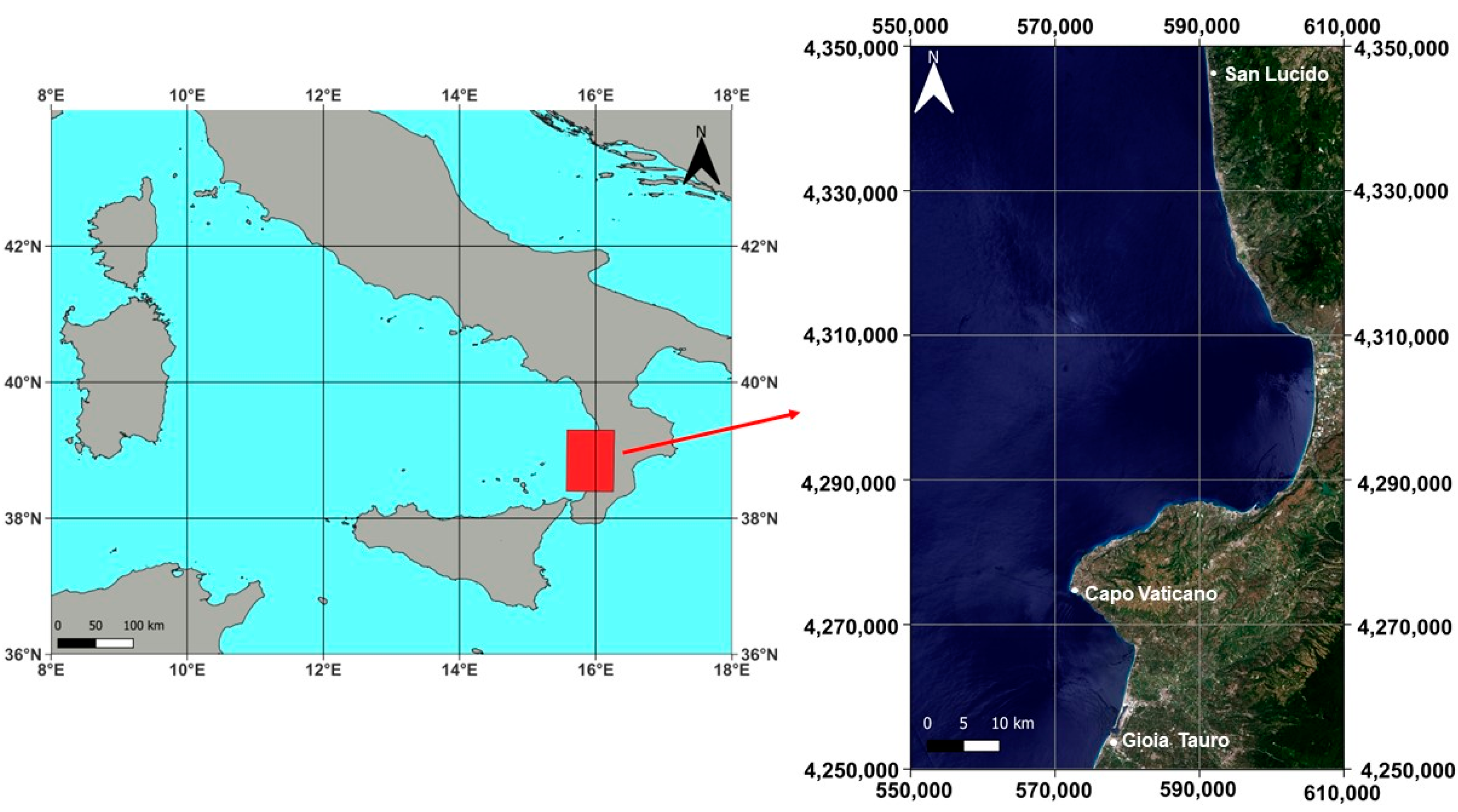
Figure 1. Study area: on the left, the location of the study area in the Tyrrhenian Sea in equirectangular projection and WGS 84 geographic coordinates (EPSG:4326); on the right, the visualization in RGB true color composition of Landsat 8 OLI images in UTM/WGS 84 plane coordinates expressed in meters (EPSG: 32632).
Remotesensing 15 03181 g001
Figure 2. Workflow of the methodological approach adopted in our study.
Remotesensing 15 03181 g002
Figure 3. False color visualization (on the left) and result of KM clustering (on the right) applied to bands 2-5-6.
Remotesensing 15 03181 g003
Figure 4. False color visualization (on the left) and result of KM clustering (on the right) applied to bands 1-3-6.
Remotesensing 15 03181 g004
Figure 5. False color visualization (on the left) and result of KM clustering (on the right) applied to bands 1-2-9.
Remotesensing 15 03181 g005
Figure 6. Geolocation of the three examined frames.
Remotesensing 15 03181 g006
Figure 7. Comparison between the reference coastline (in black) and the automatically vectorized coastline (in red) resulting from B2, B5, B6 band composition in frame 1.
Remotesensing 15 03181 g007
Figure 8. Comparison between the reference coastline (in black) and the automatically vectorized coastline (in red) resulting from B3, B4, B5 band composition in frame 1.
Remotesensing 15 03181 g008
Figure 9. Comparison between the reference coastline (in black) and the automatically vectorized coastline (in red) resulting from B3, B4, B6 band composition in frame 1.
Remotesensing 15 03181 g009
Figure 10. Comparison between the reference coastline (in black) and the automatically vectorized coastline (in red) resulting from B2, B3, B9 band composition in frame 1.
Remotesensing 15 03181 g010
Figure 11. Comparison between the reference coastline (in black) and the automatically vectorized coastline (in red) resulting from B2, B5, B6 band composition in frame 2.
Remotesensing 15 03181 g011
Figure 12. Comparison between the reference coastline (in black) and the automatically vectorized coastline (in red) resulting from B3, B4, B5 band composition in frame 2.
Remotesensing 15 03181 g012
Figure 13. Comparison between the reference coastline (in black) and the automatically vectorized coastline (in red) resulting from B3, B4, B6 band composition in frame 2.
Remotesensing 15 03181 g013
Figure 14. Comparison between the reference coastline (in black) and the automatically vectorized coastline (in red) resulting from B2, B3, B9 band composition in frame 2.
Remotesensing 15 03181 g014
Figure 15. Comparison between the reference coastline (in black) and the automatically vectorized coastline (in red) resulting from B2, B5, B6 band composition in frame 3.
Remotesensing 15 03181 g015
Figure 16. Comparison between the reference coastline (in black) and the automatically vectorized coastline (in red) resulting from B3, B4, B5 band composition in frame 3.
Remotesensing 15 03181 g016
Figure 17. Comparison between the reference coastline (in black) and the automatically vectorized coastline (in red) resulting from B3, B4, B6 band composition in frame 3.
Remotesensing 15 03181 g017
Figure 18. Comparison between the reference coastline (in black) and the automatically vectorized coastline (in red) resulting from B2, B3, B9 band composition in frame 3.
Remotesensing 15 03181 g018
Table 1. Characteristics of Landsat 8 OLI multispectral bands used in this study.
BandsWavelength
(Micrometers)
Resolution
(Meters)
1–Coastal aerosol0.43–0.4530
2–Blue0.45–0.5130
3–Green0.53–0.5930
4–Red0.64–0.6730
5–Near Infrared (NIR)0.85–0.8830
6–Short-wave infrared (SWIR 1)1.57–1.6530
7–Short-wave infrared (SWIR 2)2.11–2.2930
9–Cirrus1.36–1.3830
Table 2. Ranking using OIF.
RankingCompositionOIFRankingCompositionOIF
1B2 B5 B90.18579329B1 B7 B90.084795
2B4 B5 B90.17986830B2 B3 B60.083436
3B2 B5 B60.16186932B6 B7 B90.081616
4B2 B5 B70.16168233B4 B6 B90.079554
5B2 B6 B90.16078531B1 B2 B50.083167
6B5 B6 B90.15270934B3 B6 B90.068931
7B5 B7 B90.14973835B1 B2 B60.068889
8B1 B4 B50.14530036B1 B3 B70.067815
9B3 B5 B90.14339637B1 B4 B70.066368
10B2 B4 B50.13730738B1 B4 B90.065971
11B1 B3 B50.13706639B1 B3 B90.064266
12B1 B5 B90.13458640B4 B6 B70.059485
13B2 B7 B90.12944941B1 B2 B70.058933
14B2 B3 B50.12805142B2 B4 B70.058430
15B1 B5 B70.12750143B2 B3 B70.058208
16B4 B5 B60.12669344B3 B6 B70.055408
17B2 B6 B70.11940745B4 B7 B90.050217
18B1 B5 B60.11919846B3 B4 B60.049167
19B5 B6 B70.11227147B1 B3 B40.049148
20B4 B5 B70.11169048B2 B4 B90.047537
21B3 B5 B60.11113649B3 B7 B90.044217
22B3 B4 B50.10053150B2 B3 B90.043139
23B3 B5 B70.10015051B1 B2 B30.033455
24B1 B6 B90.09599852B3 B4 B70.032920
25B1 B4 B60.08598553B1 B2 B40.032286
26B1 B6 B70.08592554B2 B3 B40.030907
27B2 B4 B60.08548455B3 B4 B90.028967
28B1 B3 B60.08509256B1 B2 B90.022450
Table 3. Values for CF calculation.
BandsMinMaxDifference
B10.0976690.4832440.385575376
B20.0756770.5219980.446321465
B30.0551010.5762710.521169759
B40.0342420.6428150.608572632
B50.0250000.8188190.793818826
B60.0128381.3194351.306597019
B70.0087841.3144351.305651118
B90.0000000.0693340.069333822
Table 4. Ranking of band compositions using MOIF.
RankingCompositionMOIFRankingCompositionMOIF
1B2 B5 B60.13741229B1 B3 B60.062779
2B2 B5 B70.13720230B3 B6 B70.057872
3B5 B6 B70.12746831B1 B6 B90.056367
4B2 B6 B70.12173832B1 B5 B90.056020
5B4 B5 B60.11440333B4 B6 B90.052625
6B5 B6 B90.11044634B1 B4 B70.050877
7B5 B7 B90.10825035B1 B3 B70.050011
8B1 B5 B70.10561536B1 B7 B90.049761
9B4 B5 B70.10082037B1 B2 B60.049106
10B2 B6 B90.09972938B2 B4 B70.045975
11B1 B5 B60.09877539B1 B2 B50.045068
12B3 B5 B60.09711740B2 B3 B70.044105
13B4 B5 B90.08823841B3 B6 B90.043589
14B3 B5 B70.08748542B1 B2 B70.041990
15B1 B4 B50.08659743B3 B4 B60.039929
16B1 B6 B70.08586244B4 B7 B90.033202
17B2 B4 B50.08461345B3 B7 B90.027947
18B2 B5 B90.08109746B3 B4 B70.026724
19B2 B7 B90.07858847B1 B3 B40.024824
20B1 B3 B50.07769648B1 B4 B90.023386
21B2 B3 B50.07517949B1 B3 B90.020909
22B6 B7 B90.07295350B2 B4 B90.017814
23B2 B4 B60.06729051B2 B3 B40.016237
24B3 B5 B90.06616852B1 B2 B40.015503
25B1 B4 B60.06594353B1 B2 B30.015088
26B3 B4 B50.06445954B2 B3 B90.014909
27B4 B6 B70.06386355B3 B4 B90.011577
28B2 B3 B60.06324656B1 B2 B90.006744
Table 5. Statistical values of DRI for the extracted coastlines.
CompositionMOIF
Ranking
OIF
Ranking
Min (m)Max (m)Mean (m)Dev. ST. (m)RMSE (m)
B1 B2 B3 B4 B5 B6 B7 B9--0.016623.0137.65513.96715.927
B2 B5 B6130.00035.940 7.4175.2869.108
B2 B5 B7240.00038.3137.4805.4289.242
B5 B6 B73190.00043.1187.6385.2059.243
B3 B5 B612210.92781.6967.4365.5539.281
B2 B3 B521140.00082.0847.4665.7279.410
B3 B4 B526220.00082.1537.5665.6659.452
B2 B3 B628300.01683.1208.1205.1909.637
B1 B3 B629280.02383.1208.1915.1809.692
B3 B4 B643460.000623.0137.50812.44814.537
B2 B3 B954500.056952.77919.39869.36172.022
B3 B4 B955550.21110,288.66722.029318.800319.560
B1 B2 B956565.45611,580.8854280.7053341.6675430.578
B2 B5 B91810.00063.8277.2646.3099.621
B4 B5 B91320.00053.1037.6115.8149.577
Table 6. Thematic accuracy values.
CompositionMOIF
Ranking
OIF
Ranking
AccuracyWaterNo-Water
B1 B2 B3 B4 B5 B6 B7 B9--UA0.978320.96982
PA0.967570.97984
OA0.97389
B2 B5 B613UA0.980950.98108
PA0.979860.98211
OA0.98102
B2 B5 B724UA0.981310.97949
PA0.978120.98248
OA0.98037
B5 B6 B7319UA0.979380.96533
PA0.962530.98094
OA0.97202
B3 B5 B61221UA0.979830.96429
PA0.961350.98139
OA0.97168
B2 B3 B52114UA0.982130.95876
PA0.955000.98367
OA0.96977
B3 B4 B52622UA0.980190.96038
PA0.956920.98182
OA0.96975
B2 B3 B62830UA0.966210.96840
PA0.966390.96823
OA0.96734
B1 B3 B62928UA0.966340.96853
PA0.966540.96834
OA0.96747
B3 B4 B64346UA0.800910.98911
PA0.991000.76838
OA0.87626
B2 B3 B95450UA0.653350.99768
PA0.998760.50178
OA0.74261
B3 B4 B95555UA0.754700.82372
PA0.830130.74631
OA0.78693
B1 B2 B95656UA0.992860.52264
PA0.028750.99981
OA0.52924
B2 B5 B9181UA0.983160.95884
PA0.955040.98462
OA0.97029
B4 B5 B9132UA0.981540.96100
PA0.957560.98306
OA0.97071
Disclaimer/Publisher’s Note: The statements, opinions and data contained in all publications are solely those of the individual author(s) and contributor(s) and not of MDPI and/or the editor(s). MDPI and/or the editor(s) disclaim responsibility for any injury to people or property resulting from any ideas, methods, instructions or products referred to in the content.