An Epipolar HS-NCC Flow Algorithm for DSM Generation Using GaoFen-3 Stereo SAR Images

Abstract

Radargrammetry is a widely used methodology to generate the large-scale Digital Surface Model (DSM). Stereo matching is the most challenging step in radargrammetry due to the significant geometric differences and the inherent speckle noise. The speckle noise results in significant grayscale differences of the same feature points, which makes the traditional Horn–Schunck (HS) flow or multi-window zero-mean normalized cross-correlation (ZNCC) methods degrade. Therefore, this paper proposes an algorithm named Epipolar HS-NCC Flow (EHNF) for dense stereo matching, which is an improved HS flow method with normalized cross-correction constraint based on epipolar stereo images. First, the epipolar geometry is applied to resample the image to realize the coarse stereo matching. Subsequently, the EHNF method forms a global energy function to achieve fine stereo matching. The EHNF method constructs a local normalized cross-correlation constraint term to compensate for the grayscale invariance constraint, especially for the SAR stereo images. Additionally, two assessment methods are proposed to calculate the optimal cross-correlation parameter and smoothness parameter according to the refined matched point pairs. Two GaoFen-3 (GF-3) image pairs from ascending and descending orbits and the open Light Detection and Ranging (LiDAR) data are utilized to fully evaluate the proposed method. The results demonstrate that the EHNF algorithm improves the DSM elevation accuracy by 9.6% and 27.0% compared with the HS flow and multi-window ZNCC methods, respectively.

1. Introduction

Digital Surface Model (DSM) plays an important role in landscape modeling, vegetation monitoring, and visualization applications. Remote sensing imagery is an essential way to generate large-scale DSM. Synthetic aperture radar (SAR) imagery has significant advantages due to the independence of light and cloud conditions compared with optical imagery. There are four main ways to obtain three-dimensional (3-D) information from SAR images: clinometry, radargrammetry [1,2], polarimetry [3], and interferometry [4]. Among these methods, interferometry and radargrammetry are most commonly used [5,6]. Interferometry utilizes phase information to extract DSM, requiring high coherence between images. Therefore, the satellites’ angular and baseline conditions are rigorous. The temporal and geometric decorrelation limit the DSM generation by interferometry. Radargrammetry uses amplitude information of the images with different incident angles to realize elevation inversion. Therefore, radargrammetry is widely used for DSM generation in vegetation coverage areas. The radargrammetric approach was first used in the 1950s, but it is limited due to the low spatial resolution of SAR images. Then, high-resolution and multi-view SAR images became acquirable. It benefits from the widespread commercial very-high-resolution (VHR) spaceborne synthetic aperture radar systems, such as RADARSAT-2, TerraSAR-X, and COSMO-SkyMed. These systems facilitate the application of the radargrammetric stereo-mapping approach [7,8,9]. Radargrammetry consists of stereo matching and stereo orientation. However, stereo matching is the main bottleneck of radargrammetry [10] due to the stereo images having significant dissimilar geometric and grayscale differences. The geometric differences originate from the unique slant projection imaging mechanism of the SAR systems. The stereo images with the exact range resolution differ in geographic distance due to the different incident angles. Moreover, layover and foreshortening efforts change the topology relationship and cause geographic distortion. The grayscale differences are derived from the inherent speckle noise. The superposition of echoes from point targets produces either bright or dark speckles on the SAR image. Therefore, many efforts are performed to achieve accurate SAR stereo matching.

Stereo matching typically takes a coarse-to-fine method [11,12,13]. The coarse matching resamples the slave image into the master image space. The geographic differences between the stereo images are largely reduced. The fine matching achieves pixel-to-pixel dense matching and obtains a global disparity map.

The coarse matching is necessary for SAR stereo images in radargrammetry. The SAR images with low incidence angles have a smaller geographic range in the same slant resolution and vice versa. Therefore, low-incidence angle images are usually taken as master images, while high-incidence angle images are taken as slave images. The slave image needs to be resampled so that the scale can be the same as the master image. First, affine transformation [14] is introduced into coarse matching. It restricts the matching scope to a small 2-D space. Afterward, epipolar geometry [15] transforms the matching scope from a 2-D region to a 1-D line, significantly improving the efficiency and accuracy for subsequent dense matching. Epipolar geometry was first applied in photogrammetry [16]. Photogrammetry generates epipolar images based on rational polynomial coefficient (RPCs) models [17]. Due to the different imaging mechanisms, the RPCs approach for SAR epipolar geometry can only generate approximate solutions [18] or indirect solutions [19]. The radargrammetric epipolar geometry based on the range-Doppler (RD) equation model [20] is integrated into the radargrammetric workflow. Furthermore, a coarse pre-DEM epipolar geometry is proposed to further reduce the influence of geographic distortion [21,22]. Epipolar geometry aligns stereo images in the azimuth direction, and the pixel disparity only exists in the range direction.

The fine–dense stereo matching is the most critical step in radargrammetry. In general, dense matching is divided into local dense matching and global dense matching [23]. The most common method in local dense matching is zero-mean normalized cross-correlation (ZNCC) [24,25]. The ZNCC takes the “winner takes all” strategy using the point with the largest coefficient as the matched point in a specified neighborhood. However, the ZNCC method often fails in low-texture regions, and a multi-window ZNCC algorithm is proposed to increase the robustness and accuracy of ZNCC [26]. In addition, the local least-squares matching (LSM) method can obtain sub-pixel matching accuracies [22] but suffers from great computational burden and instability. The global dense matching algorithm employs comprehensive information to match stereo images. The semi-global matching (SGM) method [27,28] and the optical flow method are commonly used. The SGM algorithm compromises accuracy and computational efficiency to achieve a satisfactory effect [29]. The optical flow algorithm evaluates the pixels’ correspondence relationship to acquire the global disparity map. The Horn–Schunck (HS) optical flow method utilizes the grayscale invariance assumption and the slow change in flow vector assumption to estimate the global pixel variation [30]. The HS flow method transforms the problem of solving the flow field into minimizing the energy function. The optical flow method is also applied to other applications of SAR images, such as ice drift monitoring [31], heterogeneous image matching [32], etc.

This paper proposes an improved HS flow algorithm with the constraint of normalized cross-correlation based on epipolar stereo images, for short, the Epipolar HS-NCC Flow (EHNF) algorithm for dense stereo matching. The EHNF algorithm uses epipolar stereo images to simplify the matching dimension of the traditional HS flow method. Meanwhile, the grayscale invariance assumption is difficult to satisfy for the SAR images. We innovatively construct the normalized cross-correlation as a constraint term. The cross-correlation item focuses on the local grayscale relationship and compensates for grayscale differences in the EHNF algorithm. Moreover, we propose the parameters assessment methods for the cross-correlation parameter and smoothness parameter to realize the optimal stereo matching. The EHNF algorithm considers the characteristics of both global and local algorithms to obtain a more accurate DSM. Our study applies a coarse-to-fine matching strategy to implement the radargrammetry. First, the stereo images are coarsely aligned using epipolar geometry based on a rough DEM. Subsequently, the EHNF algorithm is applied for the dense stereo matching to obtain the disparity map. Furthermore, the Gauss–Newton iteration method achieves the stereo orientation by the disparity map, and scatter interpolation is used to obtain the final gridded DSM.

The remainder of this paper is organized as follows. In Section 2, we present the main algorithms for radargrammetry. Section 3 gives a detailed description of the experimental materials. The experimental results and the generated DSMs are presented in Section 4. A discussion is given in Section 5, and the conclusion is drawn in Section 6.

2. Methods

The flow chart of the radargrammetric DSM generation is shown in Figure 1. First, image preprocessing is performed for the stereo images to reduce the speckle noise. Then, the pre-DEM epipolar geometry resamples the slave image to achieve a coarse matching. The proposed EHNF algorithm achieves fine stereo matching and calculates a global disparity map. To evaluate the performance of the EHNF algorithm, the fine matching also applies the traditional HS flow method and the multi-window ZNCC method separately. Finally, stereo orientation is performed based on the disparity map, and the gridded stereo DSM is obtained by spatial interpolation.

2.1. Epipolar Geometry

Epipolar geometry reduces the geographic differences of stereo images to implement coarse stereo matching. The straight approximation and local conjugacy [15] are satisfied for SAR stereo images with same-side, approximately parallel satellite orbits. The former shows that epipolar lines can be approximated by a straight line, and the latter proves that all epipolar lines are parallel. These properties ensure that epipolar geometry can be applied in the radargrammetry. Moreover, the pre-DEM epipolar geometry can decrease the foreshortening effect and generate more accurate epipolar images. Therefore, the open SRTM DEM 30 m [33] is used as the pre-DEM in epipolar geometry.

Figure 2 illustrates the role of epipolar geometry. As shown in Figure 2a, the same feature points have pixel disparity in the range direction and azimuth direction of original stereo images. After epipolar registration, the two stereo images are aligned in the azimuth direction, with the only disparity in the range direction, as shown in Figure 2b. Epipolar geometry reduces the matching scope from 2-D to 1-D and improves the efficiency and robustness for dense stereo matching.

Epipolar geometry is divided into two steps: direct transformation and indirect transformation. Direct transformation is the coordinate transformation calculation from the master image coordinates $(r_m,c_m,h)$ to the ground target coordinates $\left(X_t,Y_t,Z_t\right)$. The indirect transformation is the coordinate transformation calculation from $\left(X_t,Y_t,Z_t\right)$ to the corresponding slave image coordinates $(r_s,c_s)$. $(r_m,c_m)$ and $(r_s,c_s)$ denote the range and azimuth direction coordinates in the master image and slave image, respectively. h is the pre-elevation from pre-DEM. $\left(X_t,Y_t,Z_t\right)$ denotes the actual geographic location in the WGS84 coordinate system.

The direct and indirect transformations are both achieved by the union of the RD equations and the Geodesic Ellipsoid equation. Additionally, the transformations involve the satellite variables related to image coordinates $(r,c)$. The satellite variables can be calculated with the parameters provided by the satellite data servicer. Epipolar geometry is performed on each pixel point of the master image to obtain the resampled slave image.

The RD equations are SAR satellite imaging equations. The range sphere equation and the Doppler cone equation are as follows

$$R=\left|{\mathbf{R}}_{\mathrm{s}}-{\mathbf{R}}_{\mathrm{t}}\right|=\sqrt{{\left(X_s-X_t\right)}^2+{\left(Y_s-Y_t\right)}^2+{\left(Z_s-Z_t\right)}^2}$$

(1)

$$\frac{\left({\mathbf{R}}_s-{\mathbf{R}}_{\mathrm{t}}\right)\left({\mathbf{V}}_s-{\mathbf{V}}_{\mathrm{t}}\right)}{\left|{\mathbf{R}}_s-{\mathbf{R}}_t\right|}=\frac{-f_{dc}\lambda }{2}$$

(2)

where ${\mathbf{R}}_s=\left(X_s,Y_s,Z_s\right)$ and ${\mathbf{R}}_t=\left(X_t,Y_t,Z_t\right)$ are the coordinates of the satellite sensor and ground target, ${\mathbf{V}}_s=\left(V_x,V_y,V_z\right)$ is the velocity of the satellite sensor, ${\mathbf{V}}_{\mathrm{t}}$ is the velocity of the ground target, $f_{dc}$ is the Doppler centroid frequency, and $\lambda$ is the wavelength of the satellite sensor. It is worth noting that ${\mathbf{V}}_{\mathrm{t}}$ is usually zero, and $f_{dc}$ is set to zero in the case of zero-Doppler-processed SAR data.

The Geodesic Ellipsoid equation is as follows

$$\frac{X_t^2+Y_t^2}{{\left(R_e+h\right)}^2}+\frac{Z_t^2}{R_p^2}=1$$

(3)

where $R_e$ and $R_p$ are the long and short semiaxes of the ellipsoidal model in the WGS84 coordinate system.

R is the distance between the satellite and the ground target point when the satellite photographs the ground point, which can be calculated as

$$R=R_{near}+m_{r}r$$

(4)

where $R_{near}$ is the initial slant range of the first range pixel, $m_r$ is the distance interval between unit pixels in the range direction, and r is the coordinate in the range direction.

${\mathbf{R}}_s$ and ${\mathbf{V}}_s$ are calculated by the polynomial with time t. The polynomial coefficients are fitted by the discrete position and velocity values of the satellite. The time t is determined as

$$t=t_0+\frac{c}{PRF}$$

(5)

where $t_0$ is the start moment of imaging, c is the coordinate in the azimuth position, and $PRF$ is the radar pulse repetition frequency.

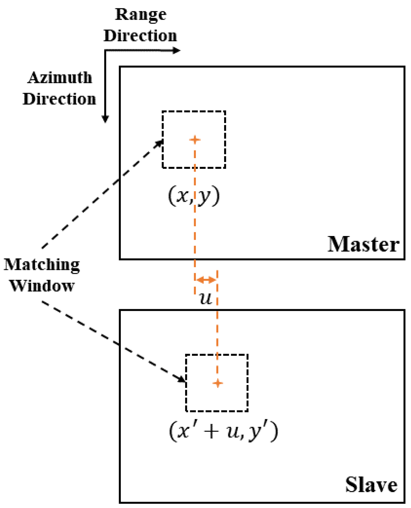
2.2. EHNF Matching Algorithm

Dense stereo matching is the most critical as it determines the DSM precision in radargrammetry. The EHNF algorithm is based on the HS flow method and combines epipolar stereo images. Additionally, the EHNF algorithm considers a local normalized cross-correlation constraint to compensate for the grayscale differences, specifically for the SAR stereo images. The EHNF algorithm achieves dense stereo matching and obtains the global pixel disparity map to realize the DSM generation.

The EHNF algorithm contains two basic assumptions: the grayscale invariance assumption and the slow change in flow vector assumption. First, the grayscale invariance assumption is that the same feature points have a similar grayscale in stereo images. The grayscale invariant constraint equation is as follows

$$I\left(x+\delta x,y+\delta y,t+\delta t\right)=I\left(x,y,t\right)$$

(6)

where $I\left(x+\delta x,y+\delta y,t+\delta t\right)$ and $I\left(x,y,t\right)$ indicate the grayscale of the master and slave image pixels, $\delta x$ and $\delta y$ are the displacements of the same feature point in the range and azimuth direction, and $\delta t$ is a unit time interval to distinguish the master image from the slave image.

For a simplified consideration, a Taylor expansion at $x,y$ is implemented as

$$I(x,y,t)=I(x,y,t)+\delta x\frac{\partial I}{\partial x}+\delta y\frac{\partial I}{\partial y}+\delta t\frac{\partial I}{\partial t}+\epsilon$$

(7)

where $\epsilon$ is the second and higher-order term containing $\delta x$, $\delta y$, and $\delta t$.

Equation (7) can subtract $I(x,y,t)$ from both sides and divide by $\delta t$ as

$$\frac{\delta x}{\delta t}\frac{\partial I}{\partial x}+\frac{\delta y}{\delta t}\frac{\partial I}{\partial y}+\frac{\partial I}{\partial t}+O\left(\delta t\right)=0$$

(8)

where $O\left(\delta t\right)$ is a small quantity containing $\delta t$.

Equation (8) can be simplified as

$$I_{x}u+I_{y}v+I_t\approx 0$$

(9)

where $I_x=\partial I/\partial x$ and $I_y=\partial I/\partial y$ are the intensity variations in the range and azimuth direction between the stereo images, respectively, $I_t=\partial I/\partial t$ is the intensity variation between the same location of the stereo images, and $u=dx/dt$ and $v=dy/dt$ are the disparities in the range and azimuth direction.

The disparity in the azimuth direction is negligible due to the epipolar resampling. Thus the conventional grayscale invariant equation can be simplified as only relating to the range direction disparity u. The item about the grayscale invariance assumption is constructed for the EHNF algorithm as

$$E_{grayscale}=\int \int \left(I_{x}u+I_t\right)dxdy.$$

(10)

In the fine matching, a global disparity map u is desired to make the master image as close as possible to the slave image, meaning the energy function in (10) should be minimized.

After epipolar geometry, the disparity variation of stereo images in the range direction is not very dramatic, so the constraint term is added to limit the change rate of the flow vector. The slow change in the flow vector assumption is as follows

$$E_{smooth}=\int \int \left({\left(\frac{\partial u}{\partial x}\right)}^2+{\left(\frac{\partial u}{\partial y}\right)}^2\right)dxdy.$$

(11)

The slow change in the flow vector assumption reduces the occurrence of mismatchings, which means that the energy function in (11) should also be minimized.

Two crucial assumptions in the EHNF algorithm are introduced as Equations (10) and (11). However, SAR stereo images do not strictly satisfy the grayscale invariance assumption due to the different imaging conditions and the speckle noise. To improve the accuracy of the traditional HS flow method, the local normalized cross-correlation is constructed as a constraint term to compensate for the grayscale differences. The EHNF algorithm can achieve more accurate stereo matching by focusing on global and local matching. It computes the NCC between the neighborhood of corresponding pixel points in the master image and the slave image as

$$\rho =\frac{Exp\left[S_1{S}_2\right]-Exp\left[S_1\right]Exp\left[S_2\right]}{\sqrt{Var\left[S_1\right]Var\left[S_2\right]}}$$

(12)

where $\rho$ is the coefficient of the matching area varying from −1 to 1, $S_1$ and $S_2$ denote the magnitude values of the master and slave images in the matching window, and $Exp\left[·\right]$ and $Var\left[·\right]$ give the mathematical expectation and variance.

The cross-correlation item is constructed as

$$E_{ncc}=\int \int \left(I_{ncc}\right)dxdy$$

(13)

where $I_{ncc}$ is the normalized cross-correlation value of the global pixels. The matching area of NCC is associated with u. Figure 3 illustrates the calculation of the cross-correction item for a point pair. $(x,y)$ and $(x^{\prime },y^{\prime })$ are the corresponding point pair of master and slave images separately. The matching center of $(x^{\prime },y^{\prime })$ changes to the $(x^{\prime }+u,y^{\prime })$ due to disparity u.

Therefore, the global energy function for the EHNF model by combining three items is as follows

$$\begin{array}{c}\hfill E_{global}=E_{grayscale}+\beta E_{ncc}+\lambda E_{\mathrm{s}mooth}\hfill \\ \hfill =\int \int \left(I_{x}u+I_t+\beta I_{ncc}+\lambda \left({\left(\frac{\partial u}{\partial x}\right)}^2+{\left(\frac{\partial u}{\partial y}\right)}^2\right)\right)dxdy\hfill \end{array}$$

(14)

where $\beta$ is the cross-correlation parameter and $\lambda$ is the smoothing parameter.

The global disparity u can be calculated by minimizing the global energy function $E_{global}$. An iterative formula is calculated as follows

$$u^{n+1}=u^n-\frac{I_x\left(I_x{u}^n+I_t+\beta I_{ncc}\right)}{\lambda +I_x^2}.$$

(15)

The iteration is terminated when the difference between the global grayscale $\varphi$ is less than a certain threshold $\epsilon$, such as $\epsilon ={10}^{-2}$ or satisfies a certain number of iteration

$$\begin{array}{c}\hfill \sum \left(\left|{\varphi }_{n+1}-{\varphi }_n\right|\right)<\epsilon \hfill \end{array}$$

(16)

where $\varphi =I_{x}u+I_t+\beta I_{ncc}$.

2.3. Parameters Assessment of the EHNF Algorithm

The EHNF algorithm has two critical parameters: cross-correlation parameter $\beta$ and the smoothing parameter $\lambda$. $\beta$ determines the role of the cross-correlation term, which is closely related to the grayscale differences of the same feature points in the whole stereo images. $\lambda$ restricts the smoothness of the flow vector, which is related to the scope of the disparity. We propose two parameter-assessment methods based on matched point pairs for $\beta$ and $\lambda$ separately. The SAR-SIFT algorithm [34] can obtain the accurately matched point pairs of stereo images, which is a feature-based matching method that is robust to the SAR images.

The cross-correlation parameter $\beta$ is calculated by the SAR-SIFT image feature points matching and the least squares calculation. First, a series of matched point pairs are acquired as $P_1,P_2,\dots ,P_n$ from the stereo images. The cross-correlation constraint compensates for the grayscale invariant term in the EHNF algorithm. We construct expression (17) about the two constraint terms based on the matched point pairs. To obtain the optimal cross-correlation parameter value, the matched feature points should satisfy

$$min\sum _{i=1}^n{(P_{ix}{u}_i+P_{it}+\beta P_{incc})}^2$$

(17)

where $P_{ix}$ is the intensity variation in the range direction of $P_i$, $P_{it}$ is the intensity variation of $P_i$, $u_i$ is the disparity calculated by the point pair $P_i$, and $P_{incc}$ is the NCC coefficient calculated by the neighborhoods of $P_i$.

$\beta$ can be calculated by the least squares fitting as

$$\beta =-{\left(P_{incc}^T{P}_{incc}\right)}^{-1}{P}_{incc}^T\left(P_{ix}{u}_i+P_{it}\right).$$

(18)

The smoothness parameter $\lambda$ is determined by the image quality. When the image is dark, unidentified, blurry, or noisy, $\lambda$ should be large and vice versa. $\lambda$ plays an essential role in controlling the trade-off between the constraint items in the EHNF algorithm. If $\lambda$ is too small, it will lead to too many mismatchings. If $\lambda$ is too large, the flow vector would be too smooth.

We apply an experimental strategy to obtain a suitable smoothness parameter value. First, the disparity of the matched point pairs is calculated from the SAR-SIFT algorithm. Then, the disparity map with different $\lambda$ is obtained in ascending order. A root mean square (RMS) is calculated between the disparities as

$$\mathrm{RMS}=\sqrt{\frac{\sum _{i=1}^n{\left(\left(p_{is}-p_{im}\right)-u_i\right)}^2}{n}}$$

(19)

where $p_{is}$ and $p_{im}$ are the coordinates in the range direction of matched points $P_i$, and $u_i$ is the corresponding disparity calculated by the EHNF algorithm.

A series of RMSs are obtained with the different $\lambda$. Considering the trade-off between the smoothness constraint and the other constraints, we choose a suitable $\lambda$ with $\mathrm{RMS}\approx 1$.

2.4. Computation of Stereo Orientation Model

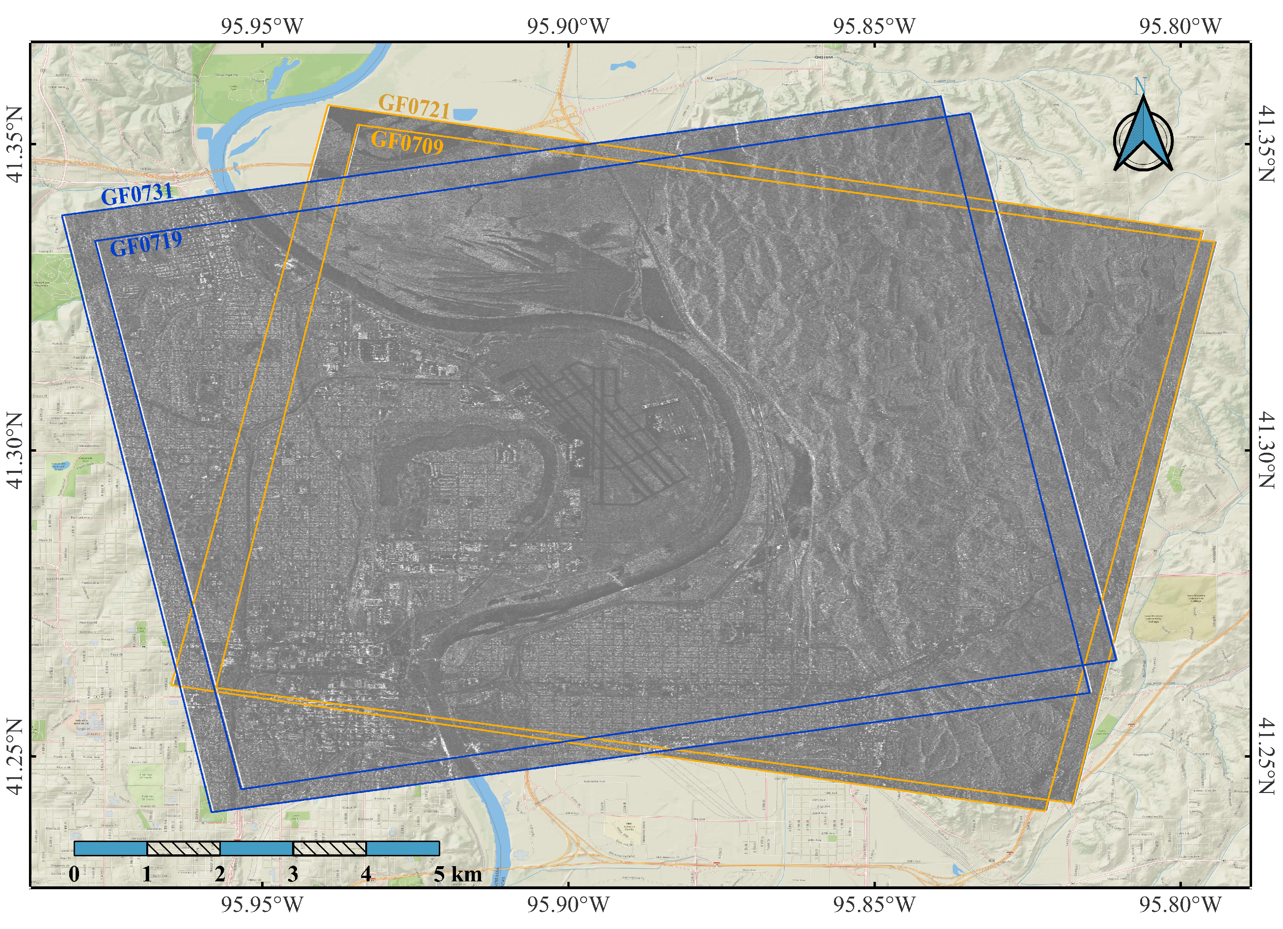
The objective of this step is to extract 3-D geometric data from the matched point pairs from the disparity map. The matched point pair has two range equations and two Doppler equations separately [35,36]. The 3-D ground point’s coordinates $(X_t,Y_t,Z_t)$ can be solved as

$$\left\{\begin{array}{c}{\mathbf{R}}_m-\sqrt{{\left(X_m-X_t\right)}^2+{\left(Y_m-Y_t\right)}^2+{\left(Z_m-Z_t\right)}^2}=0\hfill \\ \left({\mathbf{R}}_m-{\mathbf{R}}_t\right){\mathbf{V}}_m=0\hfill \\ {\mathbf{R}}_s-\sqrt{{\left(X_s-X_t\right)}^2+{\left(Y_s-Y_t\right)}^2+{\left(Z_s-Z_t\right)}^2}=0\hfill \\ \left({\mathbf{R}}_s-{\mathbf{R}}_t\right){\mathbf{V}}_s=0\hfill \end{array}\right.$$

(20)

where ${\mathbf{R}}_m=\left(X_m,Y_m,Z_m\right)$ and ${\mathbf{R}}_s=\left(X_s,Y_s,Z_s\right)$ are coordinates of the satellite sensor of the master and slave image, ${\mathbf{R}}_t=\left(X_t,Y_t,Z_t\right)$ is the coordinates of the ground target, and ${\mathbf{V}}_m,{\mathbf{V}}_s$ are the velocity of the satellite sensor of the master and slave image, respectively.

The range and Doppler equations are nonlinear and cannot be solved directly. The Gauss–Newton iteration method is applied to calculate the optimal least squares solution.

A series of discrete geographical coordinate points are obtained by computing each matched point pair with the Gauss–Newton iterative method. The inverse distance to a power method is used to acquire the gridded DSM by calculating the coordinates within a specific field for each grid point as

$${\displaystyle Z=\frac{{\displaystyle \sum _{i=1}^n\frac{z_i}{r_i^{\rho }}}}{{\displaystyle \sum _{i=1}^n\frac{1}{r_i^{\rho }}}}}$$

(21)

where $z_i$ is the intensity value of discrete geographical coordinate point i, r is the distance from point i to the grid point, n is the total number of points in the search area, and $\rho$ is the weight coefficient; usually $\rho =2$.

3. Materials

The GaoFen-3 (GF-3) satellite is a Chinese C-band multi-polarization synthetic aperture radar that belongs to the National High-Resolution Earth Observation System Major Project [37,38,39]. GF-3 has 12 different imaging modes, such as strip, spotlight, and scan modes. In addition, GF-3 has a high resolution varying from 1 to 500 m, a large imaging width ranging from 10 to 500 km, and long-life operation. As the SAR satellite can provide all-weather and all-time earth observation, it can acquire remote sensing information comprehensively and play an important role in many applications [40,41,42].

The experimental area is mountain terrain in Omaha, Nebraska, USA. The average elevation is 300 m above sea level. The area is with rich vegetation coverage and a strong decorrelation for interferometry. Therefore, it is suitable to use radargrammetry to generate DSM. Two pairs of GF-3 stereo images are selected, as shown in the blue and orange boxes in Figure 4. The mountain area in both stereo images is selected for the experiment. The mountains area has abundant image features to facilitate stereo matching. Moreover, the elevation of mountains varies significantly, which is effective in achieving a fine elevation comparison.

The stereo pairs are all spotlight-mode collected from an ascending orbit (GF0719, GF0731) and a descending orbit (GF0721, GF0709) from the different sides of the mountain. However, the images with identical orbits are on the same side. The detailed image parameters are listed in

Table 1. Basic parameters of stereo images.

ID	Satellite	Imaging Mode	Acquisition Data	Orbit Direction	Incident Angles (°)	Resolution rg/az 1 (m)
GF0719	GaoFen-3	Spotlight (SL)	2019-07-19	Ascending	25.468–26.338	0.5621/0.3126
GF0731	GaoFen-3	Spotlight (SL)	2019-07-31	Ascending	30.310–31.121	0.5621/0.3124
GF0721	GaoFen-3	Spotlight (SL)	2019-07-21	Descending	30.095–31.301	0.5621/0.3124
GF0709	GaoFen-3	Spotlight (SL)	2019-07-09	Descending	35.733–36.436	0.5621/0.3309

¹ rg represents range direction, and az represents azimuth direction.

.

The study used SRTM DEM 30 m as coarse pre-DEM to participate in epipolar resampling. SRTM DEM is an international study that obtained digital elevation models on a near-global scale. NASA JPL provides this SRTM V3 product (SRTM Plus) at a resolution of approximately 30 m. Open LiDAR data are used as actual values to verify the accuracy of the experimental results, which is from the U.S. Geological Survey (USGS) Three-Dimensional Elevation Program (3DEP) [43]. The LiDAR data started in 2020 and ended in 2021, which is close in time to the experimental SAR data. Considering that there is no remarkable topographic change in the experimental area, it is feasible to use it as accurate data for comparison.

4. Experiments and Results

4.1. Data Preprocessing

The stereo images are all in spotlight mode with a high spatial resolution. However, the orbital data of the GF-3 satellite used here are real-time. Therefore, an area block adjustment is performed to reduce the orbit error to meet the DSM generation accuracy requirements [44].

The multi-looking operation effectively reduces the speckle noise and processes fewer pixel points to obtain the same size area of DSM. In experiments, a $5\times 2$ multi-looking process is used, with a five-fold multi-looking in the azimuth direction and a two-fold multi-looking in the range direction. Although a large multi-looking operation is applied to the azimuth direction, the pixels in the azimuth direction are matched in the epipolar process, so it does not significantly impact the subsequent matching. The range direction uses only two-fold multi-looking to reserve the original image characteristics as much as possible while removing the speckle noise.

In addition, Lee filtering is also employed for stereo images. Lee filtering is a multiplicative noise model based on speckle noise. It is an adaptive filtering algorithm using the sample mean and variance information within a specific filtering window. The stereo images are performed by Lee filtering with a $5\times 5$ window.

4.2. Epipolar Geometry Processing

The pre-DEM epipolar geometry achieves the coarse matching of stereo images. We generate fusion graphs to display the results of epipolar resampling qualitatively, where a part of the ascending and descending orbits of the stereo images are shown separately in Figure 5.

Figure 5a,c are fusion images of the original stereo images from different orbits. Due to the different incident angles, the master and slave images significantly differ in range and azimuth direction. It is difficult to complete the stereo matching with the vast geographic differences. Therefore, coarse matching is essential for stereo images. Figure 5b,d are fusion images of the epipolar stereo images. Epipolar geometry aligns stereo images in the azimuth direction and evidently reduces the disparity in the range direction. The epipolar stereo images provide better materials for subsequent matching and disparity generation.

4.3. Parameters Values of Algorithms

The parameters assessment methods are introduced in Section 2.3. We calculate the accurately matched point pairs by the SAR-SIFT algorithm. The optimal value of the cross-correlation parameter $\beta$ is calculated as Equation (18). The EHNF and HS flow algorithms have the smoothness parameter $\lambda$. We calculate the RMS in Equation (19) with the different $\lambda$ in a fixed step size. The stereo images have a small-scale disparity after epipolar geometry. We set the same standard for both algorithms as the $\mathrm{RMS}\approx 1$, which is suitable to balance the smoothness item and other items verified by the experiments. Moreover, we set window sizes as $3\times 3$, $9\times 9$, and $13\times 13$ for the multi-window ZNCC algorithm. The parameter values are shown in

Table 2. Parameter values of the dense matching algorithms.

Data	Algorithm	$\mathit{\beta }$	$\mathit{\lambda }$
GF0719 & GF0731	EHNF	9.190	25
	HS	–	7
GF0721 & GF0709	EHNF	1.563	20
	HS	–	5

.

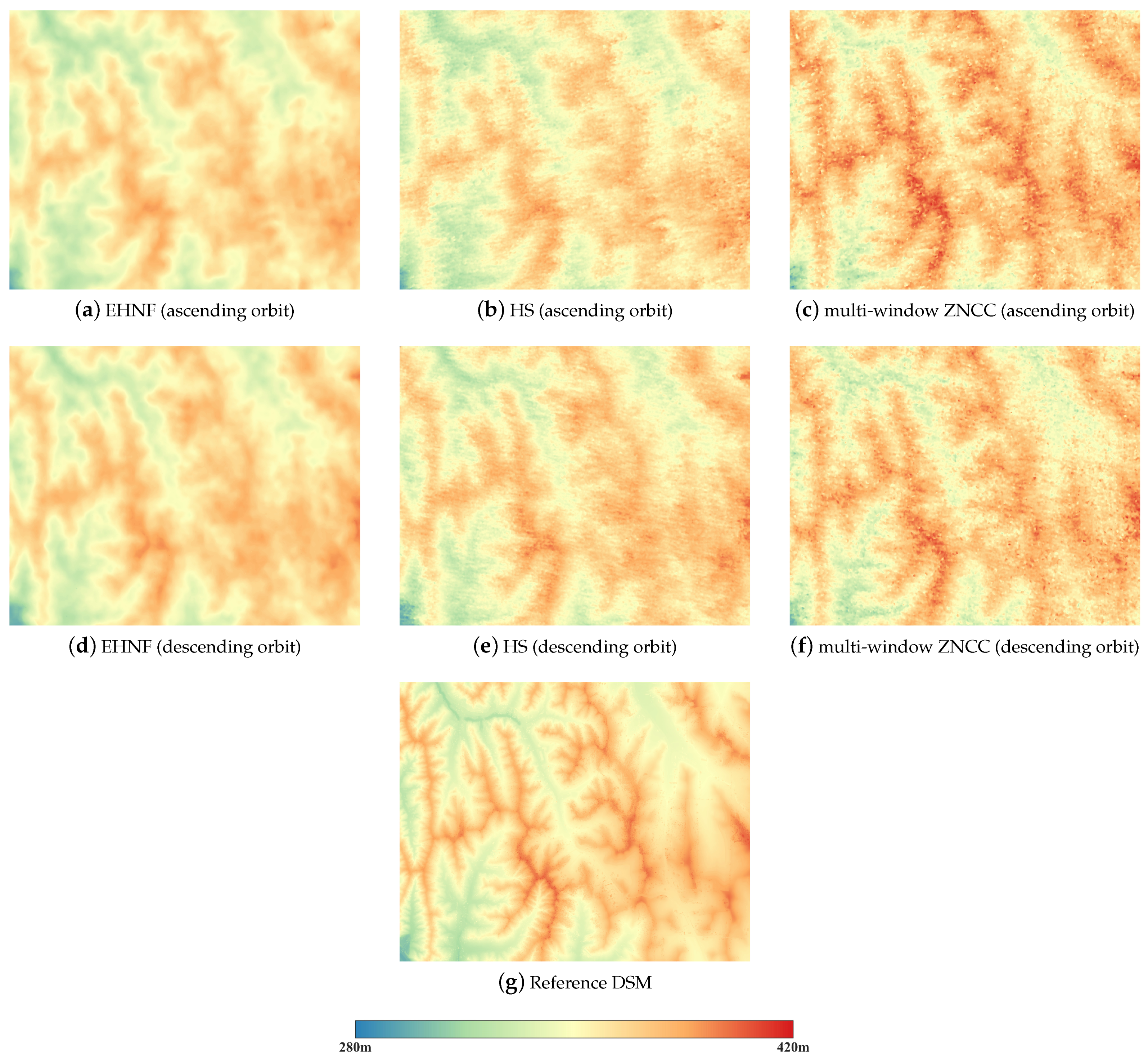
4.4. Evaluation of the Radargrammetric DSMs

The stereo images are aligned in the azimuth direction after coarse matching by the epipolar constraint. The EHNF algorithm is applied to implement the dense matching and obtain the global disparity map. The Gauss–Newton iteration and scatter interpolation are used to obtain the final gridded DSMs. In our experiments, two sets of stereo images are conducted separately. The DSMs are shown in Figure 6.

The obtained DSMs cover most of the mountain area in the stereo images. The area of ascending orbit DSM is 7.9 × 3.9 km in height and width, and that of descending orbit DSM is 6.9 × 5.1 km. The elevation varies from 280 to 420 m, which does not change violently. Moreover, the spatial resolution of DSMs is all 2 m. As the rectangles in Figure 6a, we selected mountainous and slightly flat areas for detailed analysis. Moreover, the LiDAR data are processed to obtain DSM as the standard data for comparison.

The traditional HS flow and multi-window ZNCC methods are used for algorithm comparison. The EHNF algorithm is an improved HS flow method for SAR stereo images. The traditional HS flow method is adapted to evaluate pixel displacement for optical images. The grayscale differences of SAR images make the HS flow method degraded. The multi-window ZNCC method improves the matching accuracy more than the traditional ZNCC method, and it is a classical local matching algorithm for many matching applications. We will show the results of DSMs from the different stereo-matching algorithms.

Figure 7 presents the obtained DSMs marked by the blue rectangle in Figure 6a. The mountainous geographical extent is 3078 × 2464 m. As shown in Figure 7b,e, the DSMs produced by the HS flow algorithm have slight noise compared with the EHNF algorithm due to the heavy grayscale differences among the stereo images. Many spot-like regions in Figure 7c,f manifest a poor spatial continuity of the multi-window ZNCC algorithm. The EHNF algorithm has better smoothness by considering the disparities of adjacent pixels, which is the benefit of using global information. Moreover, the DSM generated by LiDAR data shows a more precise outline than other algorithms.

To quantitatively evaluate the quality of the DSMs, two statistical metrics, mean absolute error (MAE) and root mean square error (RMSE), are chosen to evaluate the generated DSMs for the whole pixels. The MAE is the average over the map of the absolute differences between experimental and standard DSMs. The RMSE is the square root of the average squared differences between experimental and standard DSMs. Moreover, the RMSE is a frequently used measure for error measurements and is more sensitive to outliers.

The results of the two sets of stereo images are presented in

Table 3. Assessment of the elevation accuracy of mountainous DSMs.

Data	Matching Algorithm	MAE (m)	RMSE (m)
GF0719 & GF0731	EHNF	6.77	8.61
	HS	7.48	9.53
	ZNCC	9.75	11.79
GF0721 & GF0709	EHNF	5.02	6.38
	HS	5.55	7.03
	ZNCC	6.56	8.35

separately. The EHNF algorithm performs better than the traditional HS method and the multi-window ZNCC method. The HS flow method with global matching outperforms the ZNCC method with local matching. Remarkably, the EHNF algorithm improves the DSM elevation RMSE by 9.6%, 27.0% in ascending stereo images, and 9.2%, 23.6% in descending stereo images compared with the HS flow method and multi-window ZNCC method, respectively. Moreover, the DSMs generated by descending orbit images have better accuracy than that of ascending orbit images. Figure 8 presents the root square error of different algorithms to show a 2-D representation of the error. Significant errors occur at the edges of the mountain. The EHNF algorithm has fewer error points and smaller error values than the other two methods.

The elevation comparison of DSMs is also implemented for a slightly flat area, marked by the purple rectangle in Figure 6a. The DSMs are listed in Figure 9 with 1269 × 976 m. Similar to the mountain area, the DSMs generated by the EHNF algorithm have minor noise compared with that of the other methods. Moreover, the quantitative metrics are also calculated, as shown in

Table 4. Assessment of the elevation accuracy of flat DSMs.

Data	Matching Algorithm	MAE (m)	RMSE (m)
GF0719 and GF0731	EHNF	6.44	8.03
	HS	7.05	8.92
	ZNCC	9.98	12.17
GF0721 and GF0709	EHNF	4.94	6.64
	HS	5.70	7.59
	ZNCC	6.18	7.98

. The EHNF algorithm also has higher accuracy in MAE and RMSE. Moreover, the DSMs of flat areas have minor errors compared to mountainous areas. Figure 10 presents the root square error of the flat area. Similar to the mountainous area, significant errors occur at the edges. The EHNF algorithm has better results than the other two methods.

5. Disscussion

5.1. Evaluation of the EHNF Algorithm

Radargrammetric DSM generation is a complex process in which the most critical step is dense stereo matching. Recent studies have used the radargrammetry method to generate DSMs in the mountainous area. Article [29] uses the semi-global matching method with different penalty functions to generate the DSM. It provides RMSE values of 8.9–11.6 m in the mountainous area. Moreover, article [22] applies an adaptive-window least squares matching (LSM) method to generate DSMs, with RMSE values of 9.4–13.8 m in the mountainous area. The LSM method is not robust enough and it is time-consuming. The EHNF algorithm proposed in this paper implements the RMSE values of 6.64–8.03 m, which are better than the recent studies.

In previous studies, the dense matching algorithm, such as the ZNCC method [45], has achieved favorable results applied to SAR images. However, it focuses on the fixed pixel neighborhood to achieve dense matching, which largely depends on the texture condition. The mismatchings always occur and make elevation values too high or too low. The ENHF algorithm considers both global and local stereo matching. The global properties consider the disparity relationship of the adjacent pixels, which avoids significantly deviating from the actual value. Compared with the traditional HS flow algorithm, the ENHF algorithm simplifies the matching dimension by using epipolar geometry. More importantly, the EHNF algorithm improves the adaptability of SAR stereo images. It increases the cross-correlation item to compensate for the grayscale differences caused by the speckle noise. The cross-correlation item solves the problem of invalidation of the grayscale invariance assumption. However, the EHNF algorithm is calculated by iteration. The entire disparity map determines the terminated condition, which may lead to missing details in the final DSM. Moreover, the experimental results show that the EHNF algorithm has obvious accuracy advantages in evaluation metrics than the other two dense matching algorithms, reflecting the superiority of the proposed algorithm in this paper.

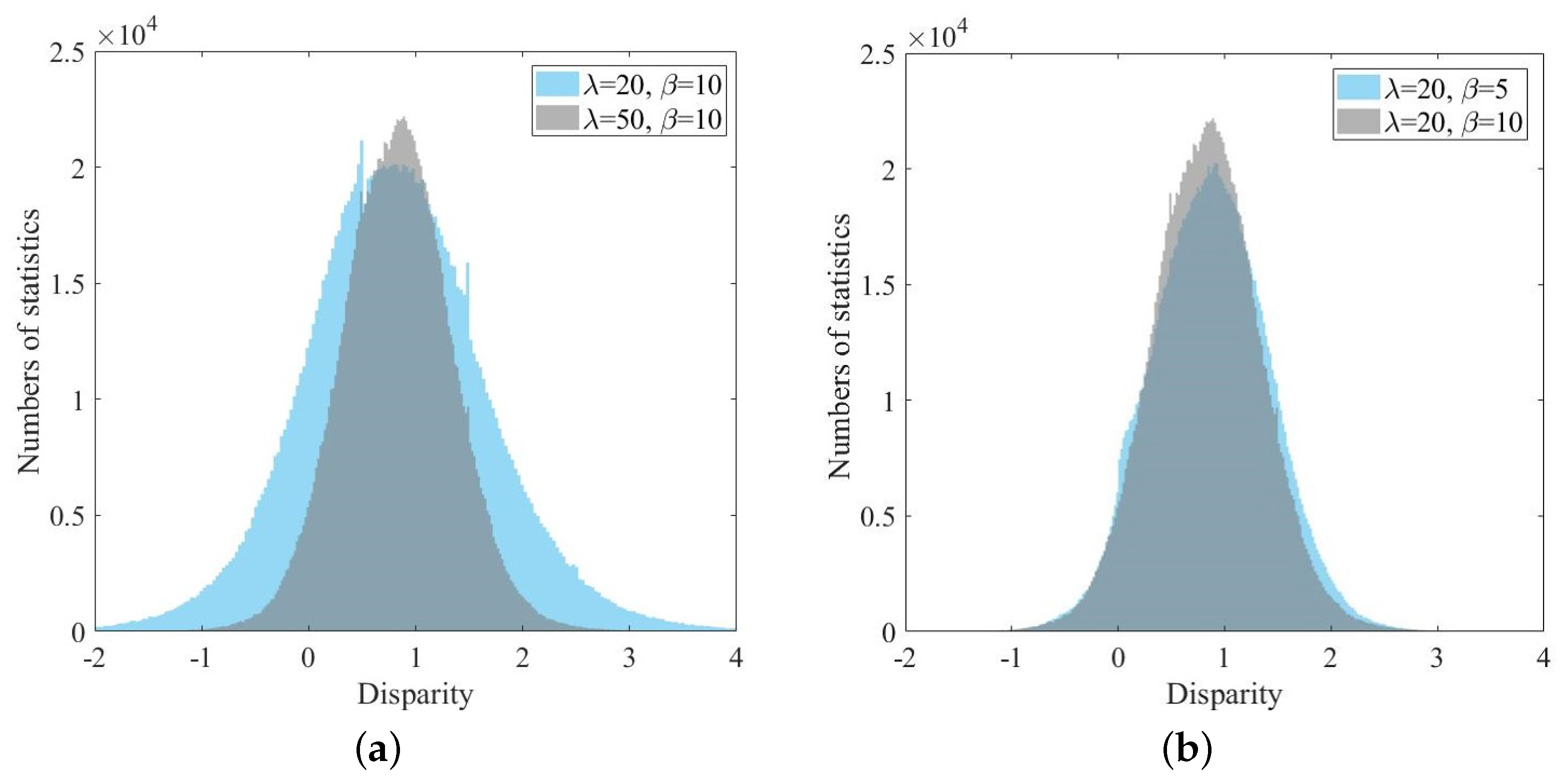
5.2. Analysis of the Impact of the EHNF Algorithm Parameters

The EHNF algorithm has two crucial parameters, the cross-correlation parameter $\beta$ and the smoothing parameter $\lambda$. $\beta$ is related to the weight of the cross-correlation constraint term. $\lambda$ determines the smoothness of the global disparity. We present the role of the two parameters through a statistical histogram of the global pixel disparities obtained from the EHNF matching algorithm. As shown in Figure 11a, with the same $\beta$, increasing $\lambda$ will result in a more concentrated distribution of disparities. For the pixels to be matched, a larger $\lambda$ results in a smaller search range and a smoother change in the disparity map and vice versa.

We explore the role of the cross-correlation parameter $\beta$ of the EHNF algorithm in Figure 11b. With the same smoothing parameter $\lambda$, the disparity distribution is more centered when $\beta$ is larger. A larger $\beta$ requires a minor disparity u to satisfy the minimization of the energy from Equation (14). Thus the greater the influence of the cross-correlation parameter, the more convergent the distribution of the disparities. However, when the cross-correlation parameter is too large, it can lead to the final result not converging. The EHNF algorithm parameters setting is closely related to the actual images to be matched.

We propose the assessment methods for the parameters separately in Section 2.3, and the optimal parameters $\beta$ and $\lambda$ are calculated based on the matched point pairs by the SAR-SIFT algorithm. The experimental results show that the EHNF algorithm with parameter assessment acquires precise DSMs. However, assessment methods are largely related to the quality of the matched point pairs and may lead to deviations by using the samples to estimate the whole image. Therefore, the assessment of the parameters is linked to the different stereo images.

5.3. Difference Analysis of the Stereo Images

Two sets of stereo pairs are used for DSM generation: the ascending orbit stereo images GF0719 and GF0731 and the descending orbit stereo images GF0721 and GF0709. The satellite’s ascending and descending orbit images are used to observe the experimental region from different sides of the mountain. As shown in Figure 12, significant differences exist in the degree of slope on the different sides of mountain areas, and the SAR images also vary widely.

The images have more pixels in the same geographical range with a high incidence angle when they have the same slant resolution in range direction. For example, Figure 12b has a larger viewing angle than Figure 12a, ${30}^{\circ }$ and ${25}^{\circ }$, respectively. More feature details can be presented in high-incidence angle images, resulting in a more accurate matching. The incidence angle range of the descending orbit stereo image pair is from ${30}^{\circ }$ to ${35}^{\circ }$, and that of the ascending orbit stereo image pair is from ${25}^{\circ }$ to ${30}^{\circ }$. In the generated mountainous DSMs, the RMSE of the descending orbit stereo image pair is 6.38 m, while that of the ascending orbit stereo image pair is 8.61 m by the EHNF algorithm. Moreover, the intersection angles of the two stereo pairs are both about five degrees. The stereo images on the same side are more similar to the smaller intersection angle, which makes the matching more accurate. In the follow-up, we can focus on the DSM generation of stereo images with different angular differences, the fusion matching of multi-angle and multi-orbit SAR images, etc.

6. Conclusions

This paper proposes an EHNF algorithm for dense stereo matching and generates high-accuracy radargrammetric DSM generation in the vegetation-covered mountain area. The EHNF algorithm realizes accurate stereo matching by optimizing the global energy function to obtain the disparity map. The EHNF method reduces the matching dimension to realize a more robust matching by the epipolar geometry. It innovatively constructs the cross-correlation item to solve the severe grayscale differences of SAR stereo images. Moreover, we propose the parameter assessment method to obtain the optimal matching result. We experiment with two pairs of stereo images to compare the EHNF algorithm with the traditional HS flow method and the multi-window ZNCC method from ascending and descending orbits stereo images. The experimental results show that the EHNF algorithm obtains more accurate elevation results using LiDAR data as the standard. In future research, dense matching algorithms with different intersection angles, different orbits, and multi-angle fusion need to be attempted to explore more precise radargrammetry.

References

1. Solberg, S.; Riegler, G.; Nonin, P. Estimating forest biomass from TerraSAR-X stripmap radargrammetry. IEEE Trans. Geosci. Remote Sens. 2014, 53, 154–161. [Google Scholar] [CrossRef]
2. Feng, S.; Lin, Y.; Wang, Y.; Yang, Y.; Shen, W.; Teng, F.; Hong, W. DEM generation with a scale factor using multi-aspect SAR imagery applying radargrammetry. Remote Sens. 2020, 12, 556. [Google Scholar] [CrossRef] [Green Version]
3. Huang, Z.; Yun, Y.; Chai, H.; Lv, X. The Iterative Extraction of the Boundary of Coherence Region and Iterative Look-Up Table for Forest Height Estimation Using Polarimetric Interferometric Synthetic Aperture Radar Data. Remote Sens. 2022, 14, 2438. [Google Scholar] [CrossRef]
4. Khan, S.; Le Calvé, S.; Newport, D. A review of optical interferometry techniques for VOC detection. Sens. Actuators Phys. 2020, 302, 111782. [Google Scholar] [CrossRef]
5. Toutin, T.; Gray, L. State-of-the-art of elevation extraction from satellite SAR data. ISPRS J. Photogramm. Remote Sens. 2000, 55, 13–33. [Google Scholar] [CrossRef]
6. Méric, S.; Fayard, F.; Pottier, É. Radargrammetric SAR image processing. In Geoscience and Remote Sensing; ResearchGate: Berlin, Germany, 2009; pp. 421–454. [Google Scholar]
7. Toutin, T.; Chenier, R. 3-D radargrammetric modeling of RADARSAT-2 ultrafine mode: Preliminary results of the geometric calibration. IEEE Geosci. Remote. Sens. Lett. 2009, 6, 282–286. [Google Scholar] [CrossRef]
8. Raggam, H.; Gutjahr, K.; Perko, R.; Schardt, M. Assessment of the stereo-radargrammetric mapping potential of TerraSAR-X multibeam spotlight data. IEEE Trans. Geosci. Remote Sens. 2009, 48, 971–977. [Google Scholar] [CrossRef]
9. Capaldo, P.; Crespi, M.; Fratarcangeli, F.; Nascetti, A.; Pieralice, F. High-resolution SAR radargrammetry: A first application with COSMO-SkyMed spotlight imagery. IEEE Geosci. Remote Sens. Lett. 2011, 8, 1100–1104. [Google Scholar] [CrossRef]
10. Ostrowski, J.; Cheng, P. DEM extraction from stereo SAR satellite imagery. In Proceedings of the IGARSS 2000—IEEE 2000 International Geoscience and Remote Sensing Symposium. Taking the Pulse of the Planet: The Role of Remote Sensing in Managing the Environment, Proceedings (Cat. No. 00CH37120), Honolulu, HI, USA, 24–28 July 2000; Volume 5, pp. 2176–2178. [Google Scholar]
11. Capaldo, P.; Crespi, M.; Fratarcangeli, F.; Nascetti, A.; Pieralice, F. DSM generation from high resolution COSMO-SkyMed imagery with radargrammetric model. Int. Arch. Photogramm. Remote Sens. Spat. Inf. Sci. 2011, 38, 239–244. [Google Scholar] [CrossRef] [Green Version]
12. Capaldo, P.; Nascetti, A.; Porfiri, M.; Pieralice, F.; Fratarcangeli, F.; Crespi, M.; Toutin, T. Evaluation and comparison of different radargrammetric approaches for Digital Surface Models generation from COSMO-SkyMed, TerraSAR-X, RADARSAT-2 imagery: Analysis of Beauport (Canada) test site. ISPRS J. Photogramm. Remote Sens. 2015, 100, 60–70. [Google Scholar] [CrossRef]
13. Nascetti, A.; Capaldo, P.; Pieralice, F.; Porfiri, M.; Fratarcangeli, F.; Crespi, M. Radargrammetric digital surface models generation from high resolution satellite SAR imagery: Methodology and case studies. In VIII Hotine-Marussi Symposium on Mathematical Geodesy; Springer: Cham, Switzerland, 2015; pp. 233–240. [Google Scholar]
14. Raggam, H.; Almer, A. Assessment of the potential of JERS-1 for relief mapping using optical and SAR data. Int. Arch. Photogramm. Remote Sens. 1996, 31, 671–676. [Google Scholar]
15. Gutjahr, K.; Perko, R.; Raggam, H.; Schardt, M. The epipolarity constraint in stereo-radargrammetric DEM generation. IEEE Trans. Geosci. Remote Sens. 2013, 52, 5014–5022. [Google Scholar] [CrossRef]
16. Cho, W.; Schenk, T.; Madani, M. Resampling digital imagery to epipolar geometry. Int. Arch. Photogramm. Remote Sens. 1993, 29, 404–408. [Google Scholar]
17. Kim, T. A study on the epipolarity of linear pushbroom images. Photogramm. Eng. Remote Sens. 2000, 66, 961–966. [Google Scholar]
18. Belgued, Y.; Hervet, E.; Marthon, P.; Lemaréchal, C.; Rognant, L.; Adragna, F. An accurate radargrammetric chain for DEM generation. Eur. Space-Agency-Publ.-ESA 2000, 450, 167–172. [Google Scholar]
19. Pan, H.; Zhang, G.; Chen, T. A general method of generating satellite epipolar images based on RPC model. In Proceedings of the 2011 IEEE International Geoscience and Remote Sensing Symposium, Vancouver, BC, Canada, 24–29 July 2011; pp. 3015–3018. [Google Scholar]
20. Curlander, J.C. Location of spaceborne SAR imagery. IEEE Trans. Geosci. Remote Sens. 1982, 359–364. [Google Scholar] [CrossRef]
21. Perko, R.; Gutjahr, K.; Krüger, M.; Raggam, H.; Schardt, M. DEM-based epipolar rectification for optimized radargrammetry. In Proceedings of the 2017 IEEE International Geoscience and Remote Sensing Symposium (IGARSS), Fort Worth, TX, USA, 23–28 July 2017; pp. 969–972. [Google Scholar]
22. Dong, Y.; Zhang, L.; Balz, T.; Luo, H.; Liao, M. Radargrammetric DSM generation in mountainous areas through adaptive-window least squares matching constrained by enhanced epipolar geometry. ISPRS J. Photogramm. Remote Sens. 2018, 137, 61–72. [Google Scholar] [CrossRef]
23. Scharstein, D.; Szeliski, R. A taxonomy and evaluation of dense two-frame stereo correspondence algorithms. Int. J. Comput. Vis. 2002, 47, 7–42. [Google Scholar] [CrossRef]
24. Oller, G.; Rognant, L.; Marthon, P. Correlation and similarity measures for SAR image matching. In SAR Image Analysis, Modeling, and Techniques VI; International Society for Optics and Photonics: Bellingham, DC, USA, 2004; Volume 5236, pp. 182–189. [Google Scholar]
25. Liu, X.; Lei, Z.; Yu, Q.; Zhang, X.; Shang, Y.; Hou, W. Multi-modal image matching based on local frequency information. EURASIP J. Adv. Signal Process. 2013, 2013, 3. [Google Scholar] [CrossRef] [Green Version]
26. Méric, S.; Fayard, F.; Pottier, É. A multiwindow approach for radargrammetric improvements. IEEE Trans. Geosci. Remote Sens. 2011, 49, 3803–3810. [Google Scholar] [CrossRef] [Green Version]
27. Hirschmuller, H. Accurate and efficient stereo processing by semi-global matching and mutual information. In Proceedings of the 2005 IEEE Computer Society Conference on Computer Vision and Pattern Recognition (CVPR’05), San Diego, CA, USA, 20–26 June 2005; Volume 2, pp. 807–814. [Google Scholar]
28. Hirschmuller, H. Stereo processing by semiglobal matching and mutual information. IEEE Trans. Pattern Anal. Mach. Intell. 2007, 30, 328–341. [Google Scholar] [CrossRef] [PubMed]
29. Wang, J.; Gong, K.; Balz, T.; Haala, N.; Soergel, U.; Zhang, L.; Liao, M. Radargrammetric DSM Generation by Semi-Global Matching and Evaluation of Penalty Functions. Remote Sens. 2022, 14, 1778. [Google Scholar] [CrossRef]
30. Horn, B.K.; Schunck, B.G. Determining optical flow. Artif. Intell. 1981, 17, 185–203. [Google Scholar] [CrossRef] [Green Version]
31. Karvonen, J. Operational SAR-based sea ice drift monitoring over the Baltic Sea. Ocean. Sci. 2012, 8, 473–483. [Google Scholar] [CrossRef]
32. Xiang, Y.; Wang, F.; Wan, L.; Jiao, N.; You, H. OS-flow: A robust algorithm for dense optical and SAR image registration. IEEE Trans. Geosci. Remote Sens. 2019, 57, 6335–6354. [Google Scholar] [CrossRef]
33. Farr, T.G.; Rosen, P.A.; Caro, E.; Crippen, R.; Duren, R.; Hensley, S.; Kobrick, M.; Paller, M.; Rodriguez, E.; Roth, L.; et al. The shuttle radar topography mission. Rev. Geophys. 2007, 45. [Google Scholar] [CrossRef] [Green Version]
34. Dellinger, F.; Delon, J.; Gousseau, Y.; Michel, J.; Tupin, F. SAR-SIFT: A SIFT-like algorithm for SAR images. IEEE Trans. Geosci. Remote Sens. 2014, 53, 453–466. [Google Scholar] [CrossRef] [Green Version]
35. Luo, Y.; Qiu, X.; Dong, Q.; Fu, K. A Robust Stereo Positioning Solution for Multiview Spaceborne SAR Images Based on the Range–Doppler Model. IEEE Geosci. Remote Sens. Lett. 2021, 19, 1–5. [Google Scholar] [CrossRef]
36. Luo, Y.; Qiu, X.; Peng, L.; Wang, W.; Lin, B.; Ding, C. A novel solution for stereo three-dimensional localization combined with geometric semantic constraints based on spaceborne SAR data. ISPRS J. Photogramm. Remote Sens. 2022, 192, 161–174. [Google Scholar] [CrossRef]
37. Guo, H. China’s Earth Observation Development. In Proceedings of the 36th International Symposium on Remote Sensing of Environment (ISRSE36), Berlin, Germany, 11–15 May 2015. [Google Scholar]
38. Ding, C.; Liu, J.; Lei, B.; Qiu, X. Preliminary exploration of systematic geolocation accuracy of GF-3 SAR satellite system. J. Radars 2017, 6, 11–16. [Google Scholar]
39. Jiao, N.; Wang, F.; You, H.; Qiu, X. Geolocation accuracy improvement of multiobserved GF-3 spaceborne SAR imagery. IEEE Geosci. Remote Sens. Lett. 2019, 17, 1747–1751. [Google Scholar] [CrossRef]
40. Deng, Y.k.; Zhao, F.j.; Wang, Y. Brief analysis on the development and application of spaceborne SAR. J. Radars 2012, 1, 1–10. [Google Scholar] [CrossRef]
41. Zhang, K.; Lv, X.; Chai, H.; Yao, J. Unsupervised SAR Image Change Detection for Few Changed Area Based on Histogram Fitting Error Minimization. IEEE Trans. Geosci. Remote Sens. 2022, 60, 1–19. [Google Scholar] [CrossRef]
42. Li, S.; Lv, X.; Ren, J.; Li, J. A Robust 3D Density Descriptor Based on Histogram of Oriented Primary Edge Structure for SAR and Optical Image Co-Registration. Remote Sens. 2022, 14, 630. [Google Scholar] [CrossRef]
43. Lidar Data from USGS 3DEP. Available online: https://apps.nationalmap.gov/downloader/#/ (accessed on 18 November 2022).
44. Wang, R.; Chai, H.; Guo, B.; Zhang, L.; Lv, X. A Novel DEM Block Adjustment Method for Spaceborne InSAR Using Constraint Slices. Sensors 2022, 22, 3075. [Google Scholar] [CrossRef]
45. Hao, X.; Zhang, H.; Wang, Y.; Wang, J. A framework for high-precision DEM reconstruction based on the radargrammetry technique. Remote Sens. Lett. 2019, 10, 1123–1131. [Google Scholar] [CrossRef]
Figure 1. Flow chart for the radargrammetric DSM generation.
Remotesensing 15 00129 g001
Figure 2. (a) The illustration of stereo images before epipolar rectification. (b) The illustration of stereo images after epipolar rectification.
Remotesensing 15 00129 g002
Figure 3. The illustration of the calculation of the cross-correction item.
Remotesensing 15 00129 g003
Figure 4. The Omaha datasets of GF-3 stereo images.
Remotesensing 15 00129 g004
Figure 5. The fusion image of (a) the original GF0719 (in green) and original GF0731 (in purple); (b) the original GF0719 (in green) and the epipolar resampled GF0731 (in purple); (c) the original GF0721 (in green) and original GF0709 (in purple); (d) the original GF0721 (in green) and the epipolar resampled GF0709 (in purple).
Remotesensing 15 00129 g005
Figure 6. (a) The DSM generated by the ascending orbit stereo images. (b) The DSM generated by the descending orbit stereo images.
Remotesensing 15 00129 g006
Figure 7. The mountainous DSM generated by the (a) EHNF algorithm; (b) HS flow algorithm; (c) multi-window ZNCC algorithm of ascending orbit stereo images, and (d) EHNF algorithm; (e) HS flow algorithm; (f) multi-window ZNCC algorithm of descending orbit stereo images; and (g) the reference DSM generated by LiDAR data.
Remotesensing 15 00129 g007
Figure 8. The root square error of mountainous DSM generated by the (a) EHNF algorithm; (b) HS flow algorithm; (c) multi-window ZNCC algorithm of ascending orbit stereo images, and (d) EHNF algorithm; (e) HS flow algorithm; (f) multi-window ZNCC algorithm of descending orbit stereo images.
Remotesensing 15 00129 g008
Figure 9. The flat DSM generated by the (a) EHNF algorithm; (b) HS flow algorithm; (c) multi-window ZNCC algorithm of ascending orbit stereo images, and (d) EHNF algorithm; (e) HS flow algorithm; (f) multi-window ZNCC algorithm of descending orbit stereo images. (g) The reference DSM generated by LiDAR data.
Remotesensing 15 00129 g009
Figure 10. The root square error of flat DSM generated by the (a) EHNF algorithm; (b) HS flow algorithm; (c) multi-window ZNCC algorithm of ascending orbit stereo images, and (d) EHNF algorithm; (e) HS flow algorithm; (f) multi-window ZNCC algorithm of descending orbit stereo images.
Remotesensing 15 00129 g010
Figure 11. The histogram of the disparity map to explore the effect of the (a) smoothing parameter λ and (b) cross-correlation parameter β .
Remotesensing 15 00129 g011
Figure 12. The mountainous area of (a) the ascending orbit image GF0719 and (b) the descending orbit image GF0721.
Remotesensing 15 00129 g012