Abstract
Pine wood nematode (PWN), Bursaphelenchus xyophilus, originating from North America, has caused great ecological and economic hazards to pine trees worldwide, especially affecting the coniferous forests and mixed forests of masson pine in subtropical regions of China. In order to prevent PWN disease expansion, the risk level and susceptivity of PWN outbreaks need to be predicted in advance. For this purpose, we established a prediction model to estimate the susceptibility and risk level of PWN with vegetation condition variables, anthropogenic activity variables, and topographic feature variables across a large-scale district. The study was conducted in Dangyang City, Hubei Province in China, which was located in a subtropical zone. Based on the location of PWN points derived from airborne imagery and ground survey in 2018, the predictor variables were conducted with remote sensing and geographical information system (GIS) data, which contained vegetation indices including normalized difference vegetation index (NDVI), normalized difference moisture index (NDMI), normalized burn ratio (NBR), and normalized red edge index (NDRE) from Sentinel-2 imagery in the previous year (2107), the distance to different level roads which indicated anthropogenic activity, topographic variables in including elevation, slope, and aspect. We compared the fitting effects of different machine learning algorithms such as random forest (RF), K-neighborhood (KNN), support vector machines (SVM), and artificial neural networks (ANN) and predicted the probability of the presence of PWN disease in the region. In addition, we classified PWN points to different risk levels based on the density distribution of PWN sites and built a PWN risk level model to predict the risk levels of PWN outbreaks in the region. The results showed that: (1) the best model for the predictive probability of PWN presence is the RF classification algorithm. For the presence prediction of the dead trees caused by PWN, the detection rate (DR) was 96.42%, the false alarm rate (FAR) was 27.65%, the false detection rate (FDR) was 4.16%, and the area under the receiver operating characteristic curve (AUC) was equal to 0.96; (2) anthropogenic activity variables had the greatest effect on PWN occurrence, while the effects of slope and aspect were relatively weak, and the maximum, minimum, and median values of remote sensing indices were more correlated with PWN occurrence; (3) modeling analysis of different risk levels of PWN outbreak indicated that high-risk level areas were the easiest to monitor and identify, while lower incidence areas were identified with relatively low accuracy. The overall accuracy of the risk level of the PWN outbreak was identified with an AUC value of 0.94. From the research findings, remote sensing data combined with GIS data can accurately predict the probability distribution of the occurrence of PWN disease. The accuracy of identification of high-risk areas is higher than other risk levels, and the results of the study may improve control of PWN disease spread.
1. Introduction
Pine wood nematode (PWN), also known as Bursaphelenchus xylophilus, is a microscopic creature that has been found worldwide. They infect pine trees and cause a condition called pine wilt disease. Such disease is fatal to pine trees, and therefore PWN outbreaks are commonly referred to as ‘smokeless fires’ [1].
PWN was first observed in North America [2] and was soon reported elsewhere in the world. It is an invasive species to many countries including China, and it has devastating impacts on those countries’ forests [3,4]. PWN has been recorded on affecting more than 15 species of Pinus, including Pinus massoniana, which is one of the most endangered species in the world [2,5]. Affected trees will show physiological and morphological changes shortly after the infection, specifically, the changes will be observed in leaf colors [6], leaf water content, and chlorophyll content [7].
While most research was focusing on understanding PWN outbreaks from physiological, molecular, or genetic studies [8,9,10], recent evidence indicates that those spatial distributions of PWN are also important in mitigating and controlling PWM outbreak. However, obtaining such information in a timely and accurate manner remains an open challenge [11,12,13]. There are currently two ways of obtaining such information. One is relying on a conventional ground survey. However, this time and labor consuming process will always lead to an under estimation of the spatial pattern due to the time lag between the observation and the event. Another way is to model the spatial patterns by using data that was remotely obtained and was relevant to the outbreak. For example, some works used topographic features [14], stand attributes [15], and landscape patterns [16,17] in the modeling of PWN spread. The justification for this is that if the response of PWN outbreak is related to those factors, a more accurate PWN spread can be estimated when the modeling function includes these factors and consider their effects. However, those contributing factors are largely inconsistent across different studies [18,19,20], and therefore a further investigation is still needed. In addition, the performance of modeling techniques can also vary dramatically depending on the application set-up (e.g., the availability of data, data size, data type), which will introduce biases into the conclusion if the appropriate techniques were not used.
In this work, we propose a framework to guide the modeling process, which helps to timely and accurately model the spatial patterns of PWN. The framework consists of five steps: (1) study design, (2) data collection, (3) data processing, (4) feature importance analysis and model development, and (5) model validation and spatial modeling. The methods used in each step can be replaced by different methods if more suitable ones are available, and we provide a recommendation based on our evaluation result and selection criteria according to our experience to look for an appropriate method. Although there are a number of works that have already used machine learning techniques and remote sensing data to model the spatial distribution of an outbreak [14,21,22,23], the existing processes may not be generalized as they provide no recommendations on how to select the methods. This paper aims to address the following questions: (1) how can machine learning algorithms perform in identifying the occurrence and mapping the distribution of PWN disease and which is the best model for predicting the probability of presence and the risk levels of PWN? (2) What factors are potential important driving factors affecting the occurrence of PWN?
Detailed descriptions about the study area, methods, results, and discussion are provided as follows.
2. Materials and Methods
2.1. Study Area
The study was conducted in the city of Dangyang, located in the western part of Hubei province, central China (30°30′23″–31°11′42″N, 111°32′42″–112°04′42″E). The city is situated in the transition zone from the Jingshan mountains to the Jianghan plain, with the elevation ranging from 37.4 m to 1083.0 m above mean sea level. Dangyang has a typical subtropical monsoon climate, with an average annual temperature and precipitations of 16.4 °C, and 992 mm, respectively. There is 68,905.5 ha of forest in this city, which accounts for 38.32% of the land (Figure 1). The forest has high species diversity and the majority of trees being Pinus massoniana Lamb. and Pinus elliottii. Since January 2017, a sub-area of the forest has been characterized as an epidemic area by the State Forestry Administration, and it reported a PWN outbreak in 2018.
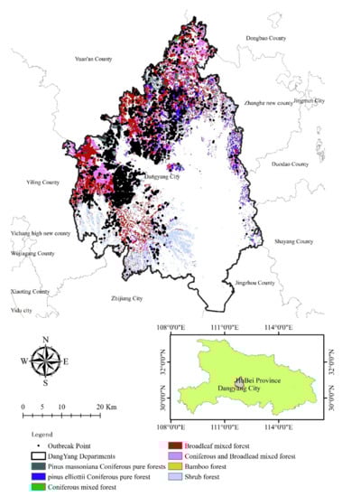
Figure 1.
Research area with different forest types.
2.2. Methods
The framework of obtaining spatial patterns of PWN outbreak is illustrated in Figure 2, which consists of five steps: (1) study design, (2) data collection, (3) data processing, (4) feature importance analysis and model development, and (5) validation and spatial modeling.
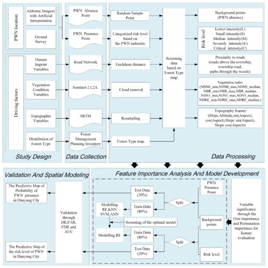
Figure 2.
Workflow chart of study which includes study design, data collection, data processing, model development, and validation.
2.2.1. Study Design
To achieve the research objects, we need the dead tree location caused by PWN and the response driving factors to these locations across the research area.
Two steps were used to acquire PWN locations over the large-scale site. First, the airborne multispectral imagery acquired on August 10, 2018, with 0.2 spatial resolution was used to derive the dead tree points by artificial interpretation, and then the ground survey was carried out to verify these points and determine the dead tree points caused by PWN at last. Due to the color and texture changes in high spatial resolution imagery, artificial interpretation is a common method in pest and disease identification [24,25,26], which can get high accuracy in detecting dead trees with a high spatial resolution (<0.5 m). The middle coordinates of the deadwood crown were recorded in the artificial interpretation. The ground survey was used to verify and remove the points which were dead trees but not caused by PWN. The ground survey was carried out from August to November in 2018, organized by the local forestry administration. On the ground survey, we went to trees identified as dead trees in remote sensing imagery and to collect the pine wood samples at 1.3 m from the base of the trunk to diagnose whether it was caused by PWN in the laboratory [1]. All the standing dead trees were checked.
In the end, the total number of dead tree points in the 2018 period caused by PWN was 19,046 as in Pinus massionana coniferous pure forests (13,122), Pinus elliottii coniferous pure forest (358), coniferous mixed forest (41), and coniferous and broad-leaf mixed forest (5525). Simultaneously, we randomly generated a similar number of background points (BK) as the absence of PWN samples in the research area. These background points (absences PWN) were all in Pinus forest types due to the PWN only presences in Pinus forest [2,5]. So, the background points located in broad-leaf mixed forest, bamboo forest, and shrub forest were removed. Finally, 2839 points were selected as background points. We assigned the value 1 and 0 for PWN points (presences) and background points (absences) respectively. At last, there were 21,885 points of PWN (presences) and background points (absences) which were obtained as the reference dataset in this paper to train and test the model.
According to the researches on the pest influence on large areas [14,21,22,27], the topographic variables, vegetation condition variables, the distribution of forest type, and human imprint variables were derived as driving factors to model the relationship with pest occurrence. In this research, we collected the topographic data, the forest type information, human imprint data, and vegetation indices which reflect the vegetation conditions to derive predictors.
2.2.2. Data Collection
Data collection is the second step of the framework, which combines raw data from different sources. The data has to cover the same spatial areas, and the temporal difference between the data should be minimized or can be justified for a reason. Three types of datasets were collected in this study as shown in Figure 2.
The geographical information system (GIS) data stands for forest management planning inventory (FMPI) data and road information. FMPI data were obtained from the local foresty administration in 2018, which contains information on forest boundary and land cover types especially contain the forest type. The roads data were collected to derive human driving factors. According to previous research, the distance roads especially to the different level roads can reflect the human activities as it has been identified as a key driving factor of PWN outbreak in existing works [2,28,29].
We collected Sentinel-2 L2A level image data to derive the vegetation indices. It was downloaded from the Google Earth Engine platform and has a spatial and temporal resolution of 20 m and five days, respectively, from the website (https://developers.google.com/earth-engine/datasets/catalog/COPERNICUS_S2_SR accessed on 18 August 2019). The L2A level data is atmospherically corrected with sen2cor algorithm and provides the bottom of atmosphere reflectance. In order to depict the gradual changes of the canopy as a contributing factor of the PWN outbreak [30], we used the image data one year before PWN outbreaks. The remote sensing image data was used to extract the vegetation index of the study area from 1 January to 31 December 2017.
To represent the topographic variables, the Shuttle Radar Topography Mission (SRTM) data were collected. The SRTM dataset is a digital elevation model (DEM) and has 30 m spatial resolution, which was obtained from the USGS website (https://earthexplorer.usgs.gov/ accessed on 18 August 2019) and used to extract topographical variables.
2.2.3. Data Processing
There are two purposes in data processing. The first is to minimize the errors inherent in the data and to extract essential information from raw data, and the second is to ensure each dataset represents one hypothetic contributing factor of PWN outbreak, which will be used for the reasoning of the potential causes of PWN outbreak.
From FMPI data, we extract the forest types boundary based on the attribution filed “species composition” in FMPI attribute table. The type of forest was classified into seven categories as Pinus massionana coniferous pure forests, Pinus elliottii coniferous pure forest, coniferous mixed forest, broad-leaf mixed forest, coniferous and broad-leaf mixed forest, bamboo forest, and shrub forest. Forest type boundary was used for the screening wood point not in the Pinus forest area.
Bases on the road information, all roads were classified into one of three categories: (a) roads above the township, (b) township roads, and (c) paths through the woods. The shortest Euclidean distances to the different levels of roads were calculated as a numeric vector. We assume that humans can access the forest through roads, and the shortest distance to different levels of roads will correlate to the different levels of human activities. Therefore, in this paper, we used the shortest distances to different levels of roads to indirectly reflect these factors.
From remote image data, we extract vegetation index using the bottom of atmosphere reflectance of sentinel-2 L2A data. First, the pixels covered by clouds were removed. Then, four spectral index indicators including normalized difference vegetation index (NDVI), normalized difference moisture index (NDMI), normalized red edge index (NDRE), and normalized burn ratio (NBR) were calculated, and we derivde the maximum, minimum, and median value of those indices from the calculation. These values of indices were selected as variables to predict PWN spatial distribution as they reflect the physiological and biochemical conditions of leaves. According to the existing work, the PWN outbreak affects the water content of pine needles and causes them to exhibit wilting symptoms [31]. Consequently, severe water stress damages the lamella structure of chloroplasts and leads to decreased chlorophyll content [32]. The NDMI and NBR were used to indicate vegetation water content [33]. In addition, NDVI and NDRE were used to reflect chlorophyll content [34].
Local topographical variables (slope, aspect, altitude) were considered as indirect factors that can impact the likelihood and severity of forest pests and disease (Mulder et al. 2020). In order to better understand the impact of topographical variables, we included slope, the aspect with sine and cosine, slope*aspect, and altitude as predictor variables in our model, which were generated from the SRTM DEM. Before calculating topographical variables, we resampled 30 m SRTM DEM to 10 m to be in line with the resolution of other variables acquired from sentinel-2 data.
The variables for predicting the PWN in this research are summarized in Table 1.

Table 1.
Variables used for predicting the PWN spatial variability.
We further categorized PWN points into five risk levels according to the number of dead trees within the 50 m radius of a point [5,16], as lower intensity (L), small intensity (S), median intensity (M), severely intensity (E), and critical intensity (C). The threshold for the number of dead trees to classify the level of risk is determined using percentile rank as 20%, 40%, 60%, 80% in the reference dataset. The risk levels of categories are presented in Table 2.
Table 2.
The number of different risk levels of PWN points.
2.2.4. Feature Importance Analysis and Model Development
The feature variables listed in Table 1 were used as input to develop the model. Firstly, the feature importance was analyzed using Gini and permutation importance analysis methods with RF model [38]. Gini importance showed the decrease in node impurity from splitting on each predictor variable, averaged over all trees in RF model [38]. Alternatively, the permutation importance analysis method evaluated how much worse the model performed when each predictor variable is assigned as random but realistic values. The worse the model performs, the more relevance that variable has in predicting [38]. After the feature importance analysis, the feature variables that showed little importance were removed.
Then, four off-the-shelf machine learning techniques were used in this study and their performance was compared. They are random forest (RF), support vector machine (SVM), K nearest neighbor (KNN), and artificial neural networks (ANN). The reasons to choose those methods are: (1) they can deal with high-dimensional datasets, (2) they have been used for modeling spatial patterns of the outbreak in other studies [39,40], and (3) they are ready to use and can be easily intergraded or implemented. The probability of PWN presence or absence (from 1 to 0) was modeled using RF, SVM, KNN, and ANN, and the performance of these models was compared. Finally, a PWN risk level was modeled by the best-fitted model in the probability of presence modeling in the last step.
RF is an ensemble machine learning (ML) algorithm for classification derived from classification and regression trees (CART) [41]. In this paper, we built RF model using the RandomForestClassifier function in the scikit-learn library (version 0.24.2) in program Python version 3.7 [38]. The main parameters in the random forest classification model are the number of subtrees (nt) and the number of predictor variables for training at each split (nf). We used ten-fold cross-validation technology to fine tune these two parameters. The nt was set from 50 to 1000 stepped by 50, and nf was set from 3 to 21 steeped by 1. The Gini importance [41] and permutation importance for feature evaluation (BRE) [38] were used to assess the importance of variables. In this paper, we obtained the best accuracy when nt was set to 500 and nf to 7.
KNN is a statistical-based classification method. KNN is an import nonparametric classification method without prior statistical knowledge, which classified input samples according to the majority of the K nearest neighbor inputs. The main parameter is the value of K. In this paper, according to the ten-fold cross-validation, we set K = 5 and use the KNeighborsClassifier function in the scikit-learn library for model building.
SVM is a supervised nonparametric statistical learning technique [42]. This method built a hyperplane with kernel function transformation imposed on input samples as a classification model. The hyperplane was determined by maximizing the distance between this hyperplane and the nearest positive and negative training samples when in the classification field [43]. In this paper, we use the radial basis function (RBF) as the kernel function. The kernel coefficient (γ) and regularization parameter (C) were the hyper-parameters for this method, the ten-fold cross-validation method was used to fine tune these parameters. The model was built using the SVC function in scikit-learn library in python. In this paper, we obtained the best accuracy when C was set to 5 and to 0.2.
ANN is a data-driven model with the ability to simulate arbitrary computing functions through optimization and has been found in a wide range of applications [44]. With back-propagation and a gradient-based optimization strategy to train a neural network with one or two hidden layers with any desired number of nodes, ANN has achieved a breakthrough in classification and regression [45]. We selected ANN due to good performance on input data in the classification field. In this paper, we chose a shallow network with one hidden layer. The model was built with MLPClassifier in scikit-learn library in python. The number of neurons in the hidden layer was set by ten-fold cross-validation from the following set: {20,50,100,200}; the optimized value was to 100 in that hidden layer.
2.2.5. Validation and Spatial Modeling
In this paper, multiple metrics were used to evaluate the performance of the methods as a single metric may not be able to illustrate the trade-offs among them. The evaluation was carried out by using randomly 20% of the samples whereas the other 80% was used to train the models and repeated five times. Detecting rate (DR), false alarm rate (FAR), false discover rate (FDR), receiver operating characteristic curve (ROC), and the area under ROC curve (AUC) were averaged five times to evaluate the accuracy.
Detection rate (DR) which is often referred to as true positive rate or sensitivity is calculated according to the Equation (1). It indicates the proportion of actually PWN points that are correctly classified as PWN points, it is equivalent to 1 minus omission error of PWN class. In addition, we used false alarm rate (FAR) to indicate the proportion of background points that the model predicted as PWN points (seen in Equation (2)) to understand the omission error of the PWN absence class. Moreover, false discovery rate (FDR) was used to assess the rate of commission error of the PWN presences class, which is defined as the proportion of all samples that were detected as PWN points but were background points (seen in Equation (3)).
DR = TP/(TP + FN),
FAR = FP/(TN + FP)
FDR = FP/(TP + FP)
Here, TP denotes the numbers of positively classified as positive; FN denotes the number of positively classified as negative; FP denotes the number of negative classified as positive; and TN denotes the number of negative classified as negative.
Generally, a high DR and a low FDR and FAR are clearly desirable, however, these cannot be fixed independently in a two-class detection problem and are both dependent on the classification threshold (T) value settled in the model. For example, in RF model, an observation assigned to a class is based on the predicted probability to this class by RF model with a set of trees voting. As if predicted probability greater than the T, the pixel was classified as presence PWN otherwise as absence one. The default T value is 0.5 in a two-class classification in RF. So, T is a key to influence the accuracy, which may influence the FAR, DR, and FDR. In this paper, we also tested how the change of T value affects the accuracy of the result, which helps to select the best T for the RF model depending on the context.
In addition, the receiver operating characteristic (ROC) curve and AUC were used to assess the overall performance of different models. ROC curve is a graph showing the performance of the classification model at all classification thresholds T, which is used to depict relative trade-offs between true positive and false positive and can be interpreted as the trade-offs between the benefit and costs [46]. In our study, ROC plots true positive rate (DR) vs. false positive rate (FAR) at different classification thresholds T. AUC is the area under ROC curve, the higher AUC, the better the performance of the model at distinguishing between the positive and negative classes. Generally, an ideal ROC cure will show the maximum benefit (true positive rate = 1) and with minimum cost (false positive = 0). Therefore, a better model will be determined as the one that is closer to the upper left corner with a higher AUC value.
After evaluating model performance, we used the best performance model for spatial modeling. The distribution of the probability of PWN presence and the PWN risk level were mapped with the best performance model.
3. Results
3.1. Variable Importance Analysis
Firstly, the Gini feature importance and the permutation feature importance of each predictor variable were tested. The results showed that the slope*cos(aspect), slope, and slope*sin(aspect), the aspect with sine and cosine, showed the least importance in test in both importance analysis methods, which indicates that the pest outbreak was less related to the slope direction among the topographic factors in this research area. Therefore, these variables were taken out from the model, and the importance of the variables of the re-fitted model is shown in Figure 3 and Figure 4. In both variable importance tests, the importance ranking results are relatively similar. We found that the distance to path through the wood and distance to township roads and the elevation and minimal value of NDVI was the most relevant explanatory variables, followed by the distance to above township roads and other vegetation indices.
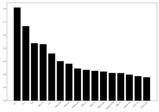
Figure 3.
Predictor variable importance with Gini importance in RF model where dis_r1, dis_r2, and dis_r3 means the distance to roads above the township, township roads, and paths through the woods, respectively.
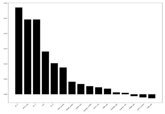
Figure 4.
Predictor variable importance with BRE importance in RF model.
3.2. Comparison of Different Models
We validated the model with AUC in ROC curve, DR, FAR, and FDR metrics using a confusion matrix. Results are shown in Table 3. The ROC curves with different models were shown in Figure 5. From Figure 5, we found RF outperforms other models since at all cut-offs the true positive rate is significantly higher and the false positive rate is lower than others. The AUC for RF is larger than other models. AUCs of RF, KNN, SVM, and ANN were 96.39%, 83.21%, 71.98%, and 70.74%, respectively.
Table 3.
Accuracy of different models in predicting PWN.
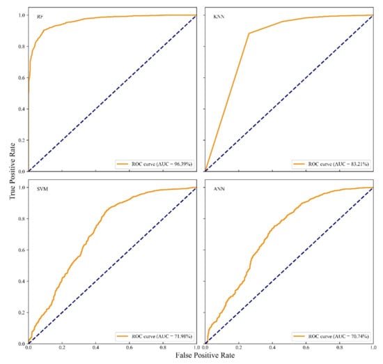
Figure 5.
ROC curve and AUC of different models with independent test data.
Considering the detecting rate, we found that all methods can produce a good result with the minimum detecting rate being 93%. The result suggests that all models can be used to detect PWN presence with acceptable performance. However, all models show a high level of false alarm rate in the results. RF model has the lowest FAR with 49.57%, and SVM has the highest FAR with 92.17%, and KNN and ANN were 60.87% and 70.08%, respectively. The results indicate that all models are more likely to classify background points to PWN points.
Considering the false discovery rate, we found that all models have good results, among which RF has the best performance (FDR = 6.66%) compared to the worst FDR = 12.32% from SVM. The results indicate that the proportion of background points which detecting as PWN points was low.
From the above analysis, we found RF model outperforms other models. Furthermore, we used the RF model to analyze how the threshold T influences the accuracy. Figure 6 presents the change of DR, FDR, FAR, and AUC with a gradual increase of threshold value using the RF model. DR was close to 1 before the threshold exceeds ~0.7, while FAR was gradually down to 0 when the threshold increased. The FDR was lower than 10% when the threshold exceeds 0.4. The threshold value was set to 0.65 in this study as it maximizes the result with DR 87.16%, FAR 6.61%, FDR 1.13%, and AUC 90.28%.
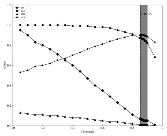
Figure 6.
Random forest model performance across the range of threshold values for PWN detection.
3.3. Analysis of Risk Levels
The classification results of different PWN risk levels are shown in Table 4. The critical class has a DR value of 84.35% and a FAR value of 2.19% and a FDR value of 9.64%, which are the highest values in these PWN risk levels. However, the background class is easily misclassified into the lower class, indicating that disease-free points are more difficult to separate with low level, but are more clearly distinguished from medium and high degree levels. On the other hand, the critical class is less likely to be misclassified, indicating that the model was able to identify signs for high disease degree. Overall, the model has a good fit with an AUC area of 93.57% (Figure 7), which indicated that the model had a good performance for risk level classification.
Table 4.
Confusion matrix of classification with RF model with different PWN risk levels.
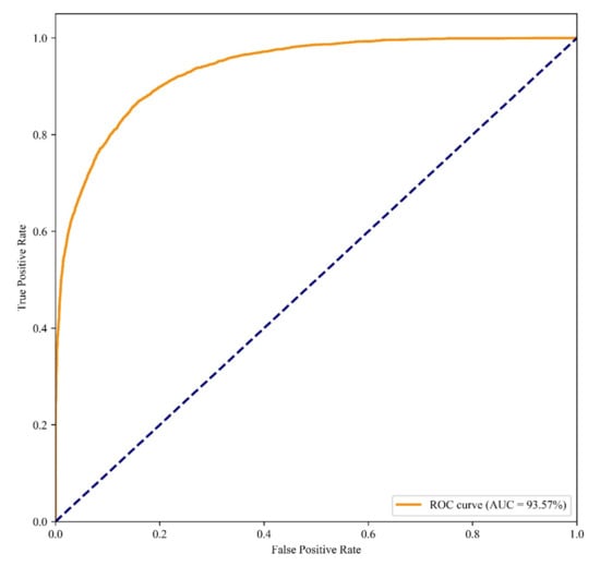
Figure 7.
ROC curve of classification with RF model with different PWN risk levels.
3.4. PWN Risk Levels Distribution in Research Area
Figure 8 presents the PWN outbreak susceptibility results showing areas with high susceptibility (1) to low susceptibility (0). Figure 9 presents the PWN risk level from lower intensity to critical intensity in the research area. The model thus identifies areas with a high probability of PWN presence in the west-central, east, and north regions of Dangyang.
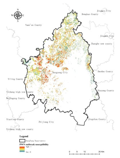
Figure 8.
The predictive map of probability of PWN presence in the research area.
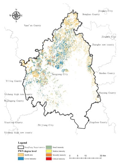
Figure 9.
The predictive map of risk levels of PWN in the research area.
The area of different PWN risk levels was shown in Table 5. We found that the area of critical risk level was lowest with 650 ha, which accounts for 1.73% in west-central regions of the study area. The non-PWN area is the highest which has 22,965 ha accounting for 61.12% of the research area. The lower, small, median, and severely level areas are 10,347 ha, 1858 ha, 1150 ha, and 607 ha, with the proportion being 27.53%, 4.94%, and 3.06%, respectively.
Table 5.
Summary area and proportion of different PWN risk levels in the research area.
4. Discussion
4.1. Analysis and Optimization of the Predictor Variables
From our results, we found that the distance to roads is an important predictor variable to model the PWN susceptibility. The distance to the roads reflected the human activities to some extent (i.e., closer to roads indicates more human activities). The results of some studies suggest that the spread of PWN on a large regional scale is to some extent due to human activities when transportation of woods such as containers, timber transportation, and power line erection [2]. The same results were found in the study in the Dangyang area, where the location of diseased wood was highly correlated with the distance of the road. We found that distance to roads is an important variable to PWN outbreak, especially to the road of the path in woods which indicates the pest outbreak is more related to human activities in this research area. This result is consistent with other research [28,29]. Based on the results of the study, it is inferred that the source of the initial PWN disease in the region may have been brought in by anthropogenic activities.
Moreover, our results show that elevation is highly related to the probability of occurrence of PWN, but the slope and slope orientation, as well as factors calculated from slope orientation, has little impact. This finding is not inline with other studies [14], and a possible reason is that the relative variation of slope and aspect in the study area is larger, and the location of PWN infestation in this study area is major distributed from slope of 0 to 30°, and the aspect is distributed from 0–360°, so it is difficult to find the relevant pattern. In addition, the spatial resolution and accuracy of DEM may influence the result. In our study, the spatial resolution of DEM was relatively lower than the Sentinel image data. Thus, the slope and aspect of the diseased wood were relatively coarse. We hypothesize that higher precision topographic data might have some influence on the results.
Different vegetation indices with maximum, minimum, and median values in a year are related to the occurrence of PWN; the minimum value of NDVI, the median value of NBR index, and the maximum value of NDMI were found to be especially related to the occurrence of PWN. The reason for this might be that the vegetation index can reflect the state of vegetation after disturbance to some extent, or that the vegetation index of time series can better reflect the state of vegetation after disturbance [37,47,48], the disturbance of PWN will cause the pine tree leaves to turn red, wilt, and drop, etc. and these changes will affect the change of remote sensing signal at canopy level in turn. By selecting the maximum, minimum, and median values of vegetation index in a year, one can better reflect the changes of the disturbance information of the canopy. When the pattern of canopy change caused by PWN and other disturbance events such as the windstorm or fire can be distinguished, we can use these vegetation indices to better reflect the change of canopy state and respond to the influence of PWN disturbance more effectively.
4.2. Models Performance and Evaluation
Machine learning methods have been widely applied to a variety of classification and regression modeling. The performance and effectiveness of models are the main issues to be concerning for specific application problems. In the paper, four typical machine learning methods were compared, among which SVM and RF are currently top choices, as they were often used as baseline methods to compare and analyze with other models. KNN is a traditional method, considering the nearest neighbor feature also has a wide range of applications. ANN uses perceptron model, combined with feedback neuron network to solve the model parameters, although only a shallow network model is utilized, it performs well in solving some nonlinear problems. Although the deep learning model based on the neural network may have better performance when the training data is sufficiently large, we did not use it in this study considering the number of data samples may not be sufficient. SVM uses kernel function for space mapping method, which can solve small sample classification and regression, but the performance in this paper is not outstanding. KNN method considers the nearest neighbor feature and achieves better results in the prediction of PWN. This may be related to the spread pattern of PWN in the local area. In the local area, PWN spread is mainly caused by the migration of the host of PWN in the local area, which will form a local aggregation effect and make the pine canopy in the local near-neighborhood area construct similar disturbance characteristics. This leads to producing better results when using the KNN method than SVM and ANN. The RF approach shows the best results in our study. As with random sampling of features and samples through a bootstrap sampling strategy, it is a good solution to the overfitting problem. Although the RF model performs well overall, the results are also affected by the imbalance between positive and negative samples, resulting in a relatively high FAR.
4.3. Threshold for Model
Classification threshold plays a significant effect on the final monitoring accuracy of the RF model. Generally, a high DR and a low FDR, and a FAR are clearly desirable in PWN detecting. However, these cannot be fixed independently in two-class detection problems and both depend on the threshold value. The classification threshold represents a trade-off between true and false detection. How to balance DR, FAR, and FDR depend on the context. Generally, a viable detection method would expect to achieve a DR > 50% while limiting FDR < 20%, and FAR < 20%. Our results found that the FDR was low (<13%) at all thresholds, with DR > 90% at thresholds up to 0.8, but the FAR was more changeable, basically decreasing gradually with the increasing of the threshold, such as 47.2% at a threshold of 0.5, and FAR < 20% when the threshold was greater than 0.75 in generally. This shows that the model is prone to misclassify non-diseased wood as diseased wood. The adjustment of the threshold value can reduce the FAR while maintaining the relative stability of DR and FDR.
4.4. The Risk Level of PWN Classification
Overall, it is still difficult to identify different PWN risk levels using remote sensing data combined with topography and human activity factors. According to our results, we found that the overall accuracy is not high. Although the identification accuracy of high risk level areas was high, the low risk level areas were not easily identified. Since the low risk level area did not differ much from the no infection areas in the input features. There are some factors to influence these results. The accuracy of the risk level samples from the ground investigation may influence the results. In our research, we used the number of diseased wood neighborhood points to measure the intensity of disease occurrence location to reflect the risk levels of PWN spread to some extent. The distance to the neighborhood PWN points may impact the risk level determination. Moreover, the forest stand structural features such as species composition and stand age structure may also influence the results [49]. These factors need to be considered in future studies, which may make it easier to identify disease risk levels.
5. Conclusions
Probabilistic prediction of PWN susceptibility is important for monitoring forest health status, especially Masson pine in the subtropic zone. In this paper, the modeling of PWN outbreak probability and risk level mapping was implemented using remote sensing vegetation index, topography, and human activities variables. The main conclusions drawn are as follows:
- (1)
- It is possible to achieve the prediction probability of the presence of PWN in a large extended area with remote sensing data combined with topography, anthropogenic activities, and other variables. The overall DR can be up to 96%, FAR lower than 28%, FDR lower than 5%. Moreover, different risk levels of PWN have a certain predictive effect, especially for areas with a high risk level. Different predictor variables have different effects on PWN susceptibility, and in the Dangyang region, PWN outbreaks are highly correlated with anthropogenic activity factors.
- (2)
- Different models have different performances on the prediction of PWN. The performance of the different models is sensitive to many factors as shown in our evaluation, such as the selection of hyper-parameter, the use of training and testing datasets. In this study, we found that the RF method consistently outperforms other models that we used. Therefore, we recommend using RF first in similar applications, and only tires other models if the FR cannot provide the modeling result with sufficient accuracy.
- (3)
- The threshold value plays an important role in model performance, which balances the trade-off between true and false detection rates. However, the selection of optimal threshold value will depend on the context and can be difficult, similar to selecting optimal hyperparameters for a machine learning algorithm.
- (4)
- The predictor variables showed different importance in predicting PWN. The distance to path through the wood and distance to township roads and the elevation and minimal value of NDVI were was the most relevant explanatory variables, followed by the distance to above township roads, and other vegetation indices, the topographic variables such as slope, aspect showed the least importance. Based on the results of the study, it is inferred that the source of the initial PWN disease in the region may have been brought in by anthropogenic activities.
Author Contributions
Conceptualization, Y.D.; data curation, J.Z.; formal analysis, Y.Z., Y.H., L.H. and Z.H., S.P.; funding acquisition, Y.D.; methodology, Y.Z. and Z.H.; supervision, Y.D. and H.C.; writing the original draft, Y.Z. and Y.D.; writing–review and editing, Y.D. and X.F. All authors have read and agreed to the published version of the manuscript.
Funding
This research was funded by the National Natural Science Foundation of China (Grant No. 32071683).
Conflicts of Interest
The authors declare no conflict of interest.
References
- Suzuki, K. PATHOLOGY|Pine Wilt and the Pine Wood Nematode. Encyclopedia of Forest Sciences; Elsevier: Amsterdam, The Netherlands, 2004; pp. 773–777. [Google Scholar]
- Mota, M.M.; Vieira, P. (Eds.) Pine Wilt Disease: A Worldwide Threat to Forest Ecosystems; Springer: Dordrecht, The Netherlands, 2008. [Google Scholar]
- Hulme, P.E. Trade, transport and trouble: Managing invasive species pathways in an era of globalization. J. Appl. Ecol. 2009, 46, 10–18. [Google Scholar] [CrossRef]
- Perrings, C.; Dehnen-Schmutz, K.; Touza, J.; Williamson, M. How to manage biological invasions under globalization. Trends Ecol. Evol. 2005, 20, 212–215. [Google Scholar] [CrossRef] [PubMed]
- Juan, S.; Youqing, L.; Haiwei, W.; Heliovaara, K.; Lizhuang, L. Impact of the invasion by Bursaphelenchus xylophilus on forest growth and related growth models of Pinus massoniana population. Acta Ecol. Sin. 2008, 28, 3193–3204. [Google Scholar] [CrossRef]
- Ferrenberg, S. Landscape Features and Processes Influencing Forest Pest Dynamics. Curr. Landsc. Ecol. Rep. 2016, 1, 19–29. [Google Scholar] [CrossRef][Green Version]
- Fonseca, L.; Cardoso, J.; Lopes, A.; Pestana, M.; Abreu, F.; Nunes, N.; Mota, M.; Abrantes, I. The pinewood nematode, Bursaphelenchus xylophilus, in Madeira Island. Helminthologia 2012, 49, 96–103. [Google Scholar] [CrossRef]
- Lee, S.G.; Chung, M.S.; DeMarsilis, A.J.; Holland, C.K.; Jaswaney, R.V.; Jiang, C.; Kroboth, J.H.; Kulshrestha, K.; Marcelo, R.Z.; Meyyappa, V.M.; et al. Structural and biochemical analysis of phosphoethanolamine methyltransferase from the pine wilt nematode Bursaphelenchus xylophilus. Mol. Biochem. Parasitol. 2020, 238, 111291. [Google Scholar] [CrossRef]
- Kim, A.Y.; Osabutey, A.F.; Yoon, K.A.; Choi, B.-H.; Lee, S.-H.; Han, H.R.; Koh, Y.H. Identification of Aldose Reductase 1 as a pine wood nematode secretory enzyme and generation and characterization of its monoclonal antibodies. J. Asia-Pac. Èntomol. 2018, 22, 233–238. [Google Scholar] [CrossRef]
- Chiluwal, K.; Roh, G.H.; Kim, J.; Park, C.G. Acaricidal activity of the aggregation pheromone of Japanese pine sawyer against two-spotted spider mite. J. Asia-Pac. Èntomol. 2019, 23, 86–90. [Google Scholar] [CrossRef]
- Gastón, A.; Viñas, J.I.G. Modelling species distributions with penalised logistic regressions: A comparison with maximum entropy models. Ecol. Model. 2011, 222, 2037–2041. [Google Scholar] [CrossRef]
- Louis, M.; Toffin, E.; Gregoire, J.-C.; Deneubourg, J.-L. Modelling collective foraging in endemic bark beetle populations. Ecol. Model. 2016, 337, 188–199. [Google Scholar] [CrossRef]
- Bonneau, M.; Johnson, F.A.; Romagosa, C.M. Spatially explicit control of invasive species using a reaction–diffusion model. Ecol. Model. 2016, 337, 15–24. [Google Scholar] [CrossRef]
- Mulder, O.; Sleith, R.; Mulder, K.; Coe, N.R. A Bayesian analysis of topographic influences on the presence and severity of beech bark disease. For. Ecol. Manag. 2020, 472, 118198. [Google Scholar] [CrossRef]
- Kamińska, A.; Lisiewicz, M.; Kraszewski, B.; Stereńczak, K. Habitat and stand factors related to spatial dynamics of Norway spruce dieback driven by Ips typographus (L.) in the Białowieża Forest District. For. Ecol. Manag. 2020, 476, 118432. [Google Scholar] [CrossRef]
- Calvão, T.; Duarte, C.M.; Pimentel, C.S. Climate and landscape patterns of pine forest decline after invasion by the pinewood nematode. For. Ecol. Manag. 2019, 433, 43–51. [Google Scholar] [CrossRef]
- Ikegami, M.; Jenkins, T.A. Estimate global risks of a forest disease under current and future climates using species distribution model and simple thermal model—Pine Wilt disease as a model case. For. Ecol. Manag. 2018, 409, 343–352. [Google Scholar] [CrossRef]
- Togashi, K.; Jikumaru, S. Evolutionary change in a pine wilt system following the invasion of Japan by the pinewood nematode, Bursaphelenchus xylophilus. Ecol. Res. 2007, 22, 862–868. [Google Scholar] [CrossRef]
- Syifa, M.; Park, S.-J.; Lee, C.-W. Detection of the Pine Wilt Disease Tree Candidates for Drone Remote Sensing Using Artificial Intelligence Techniques. Engineering 2020, 6, 919–926. [Google Scholar] [CrossRef]
- Wu, B.; Liang, A.; Zhang, H.; Zhu, T.; Zou, Z.; Yang, D.; Tang, W.; Li, J.; Su, J. Application of conventional UAV-based high-throughput object detection to the early diagnosis of pine wilt disease by deep learning. For. Ecol. Manag. 2021, 486, 118986. [Google Scholar] [CrossRef]
- Vasquez, M.C.V.; Chen, C.-F.; Lin, Y.-J.; Kuo, Y.-C.; Chen, Y.-Y.; Medina, D.; Diaz, K. Characterizing spatial patterns of pine bark beetle outbreaks during the dry and rainy season’s in Honduras with the aid of geographic information systems and remote sensing data. For. Ecol. Manag. 2020, 467, 118162. [Google Scholar] [CrossRef]
- Assal, T.; Sibold, J.; Reich, R. Modeling a Historical Mountain Pine Beetle Outbreak Using Landsat MSS and Multiple Lines of Evidence. Remote Sens. Environ. 2014, 155, 275–288. [Google Scholar] [CrossRef]
- Hu, G.; Yin, C.; Wan, M.; Zhang, Y.; Fang, Y. Recognition of diseased Pinus trees in UAV images using deep learning and AdaBoost classifier. Biosyst. Eng. 2020, 194, 138–151. [Google Scholar] [CrossRef]
- Sylvain, J.-D.; Drolet, G.; Brown, N. Mapping dead forest cover using a deep convolutional neural network and digital aerial photography. ISPRS J. Photogramm. Remote Sens. 2019, 156, 14–26. [Google Scholar] [CrossRef]
- Senf, C.; Seidl, R.; Hostert, P. Remote sensing of forest insect disturbances: Current state and future directions. Int. J. Appl. Earth Obs. Geoinf. 2017, 60, 49–60. [Google Scholar] [CrossRef] [PubMed]
- Hall, R.; Castilla, G.; White, J.; Cooke, B.; Skakun, R. Remote sensing of forest pest damage: A review and lessons learned from a Canadian perspective. Can. Èntomol. 2016, 148, S296–S356. [Google Scholar] [CrossRef]
- Eitel, J.U.H.; Vierling, L.A.; Litvak, M.E.; Long, D.S.; Schulthess, U.; Ager, A.A.; Krofcheck, D.J.; Stoscheck, L. Broadband, red-edge information from satellites improves early stress detection in a New Mexico conifer woodland. Remote Sens. Environ. 2011, 115, 3640–3646. [Google Scholar] [CrossRef]
- Shin, S.-C. Pine Wilt Disease in Korea. In Pine Wilt Disease; Zhao, B.G., Futai, K., Sutherland, R.J., Takeuchi, Y., Eds.; Springer: Tokyo, Japan, 2008; pp. 26–32. [Google Scholar]
- Yang, Z.-Q.; Wang, X.; Zhang, Y.-N. Recent advances in biological control of important native and invasive forest pests in China. Biol. Control 2014, 68, 117–128. [Google Scholar] [CrossRef]
- Hansen, M.C.; Potapov, P.V.; Moore, R.; Hancher, M.; Turubanova, S.A.; Tyukavina, A.; Thau, D.; Stehman, S.V.; Goetz, S.J.; Loveland, T.R.; et al. High-resolution global maps of 21st-century forest cover change. Science 2013, 342, 850–853. [Google Scholar] [CrossRef]
- Kenji, F.; Taizo, H.; Kazuo, S. Photosynthesis and Water Status of Pine-Wood Nematode-Infected Pine Seedlings. J. Jpn. For. Soc. 1992, 74, 1–8. [Google Scholar] [CrossRef]
- Zarco-Tejada, P.; Hornero, A.; Beck, P.; Kattenborn, T.; Kempeneers, P.; Hernández-Clemente, R. Chlorophyll content estimation in an open-canopy conifer forest with Sentinel-2A and hyperspectral imagery in the context of forest decline. Remote Sens. Environ. 2019, 223, 320–335. [Google Scholar] [CrossRef] [PubMed]
- Jin, S.; Sader, S.A. Comparison of time series tasseled cap wetness and the normalized difference moisture index in detecting forest disturbances. Remote Sens. Environ. 2005, 94, 364–372. [Google Scholar] [CrossRef]
- Datt, B. Remote Sensing of Chlorophyll a, Chlorophyll b, Chlorophyll a+b, and Total Carotenoid Content in Eucalyptus Leaves. Remote Sens. Environ. 1998, 66, 111–121. [Google Scholar] [CrossRef]
- Gao, B.-C. NDWI—A normalized difference water index for remote sensing of vegetation liquid water from space. Remote Sens. Environ. 1996, 58, 257–266. [Google Scholar] [CrossRef]
- White, J.; Wulder, M.; Hermosilla, T.; Coops, N.C.; Hobart, G.W. A nationwide annual characterization of 25 years of forest disturbance and recovery for Canada using Landsat time series. Remote Sens. Environ. 2017, 194, 303–321. [Google Scholar] [CrossRef]
- Verbesselt, J.; Hyndman, R.; Newnham, G.; Culvenor, D. Detecting trend and seasonal changes in satellite image time series. Remote Sens. Environ. 2010, 114, 106–115. [Google Scholar] [CrossRef]
- Breiman, L. Random forests. Mach. Learn. 2001, 45, 5–32. [Google Scholar] [CrossRef]
- Fassnacht, F.E.; Latifi, H.; Ghosh, A.; Joshi, P.K.; Koch, B. Assessing the potential of hyperspectral imagery to map bark beetle-induced tree mortality. Remote Sens. Environ. 2014, 140, 533–548. [Google Scholar] [CrossRef]
- Dash, J.P.; Watt, M.; Pearse, G.D.; Heaphy, M.; Dungey, H. Assessing very high resolution UAV imagery for monitoring forest health during a simulated disease outbreak. ISPRS J. Photogramm. Remote Sens. 2017, 131, 1–14. [Google Scholar] [CrossRef]
- Gordon, A.D.; Breiman, L.; Friedman, J.H.; Olshen, R.A.; Stone, C.J. Classification and Regression Trees. Biometrics 1984, 40, 874. [Google Scholar] [CrossRef]
- Chang, C.-C.; Lin, C.-J. LIBSVM. ACM Trans. Intell. Syst. Technol. 2011, 2, 1–27. [Google Scholar] [CrossRef]
- Mountrakis, G.; Im, J.; Ogole, C. Support vector machines in remote sensing: A review. ISPRS J. Photogramm. Remote Sens. 2011, 66, 247–259. [Google Scholar] [CrossRef]
- Xu, Z.; Huang, X.; Lin, L.; Wang, Q.; Liu, J.; Yu, K.; Chen, C. BP neural networks and random forest models to detect damage by Dendrolimus punctatus Walker. J. For. Res. 2018, 31, 107–121. [Google Scholar] [CrossRef]
- Zhang, G.; Patuwo, B.E.; Hu, M.Y. Forecasting with artificial neural networks:: The state of the art. Int. J. Forecast. 1998, 14, 35–62. [Google Scholar] [CrossRef]
- Carrington, A.M.; Fieguth, P.W.; Qazi, H.; Holzinger, A.; Chen, H.H.; Mayr, F.; Manuel, D.G. A new concordant partial AUC and partial c statistic for imbalanced data in the evaluation of machine learning algorithms. BMC Med. Inform. Decis. Mak. 2020, 20, 4. [Google Scholar] [CrossRef]
- Spruce, J.P.; Sader, S.; Ryan, R.E.; Smoot, J.; Kuper, P.; Ross, K.; Prados, D.; Russell, J.; Gasser, G.; McKellip, R. Assessment of MODIS NDVI time series data products for detecting forest defoliation by gypsy moth outbreaks. Remote Sens. Environ. 2011, 115, 427–437. [Google Scholar] [CrossRef]
- Pasquarella, V.J.; Bradley, B.A.; Woodcock, C.E. Near-Real-Time Monitoring of Insect Defoliation Using Landsat Time Series. Forests 2017, 8, 275. [Google Scholar] [CrossRef]
- Wang, B.; Tian, C.; Liang, Y. Mixed effects of landscape structure, tree diversity and stand’s relative position on insect and pathogen damage in riparian poplar forests. For. Ecol. Manag. 2020, 479, 118555. [Google Scholar] [CrossRef]
Publisher’s Note: MDPI stays neutral with regard to jurisdictional claims in published maps and institutional affiliations. |
© 2021 by the authors. Licensee MDPI, Basel, Switzerland. This article is an open access article distributed under the terms and conditions of the Creative Commons Attribution (CC BY) license (https://creativecommons.org/licenses/by/4.0/).