
SAR Ship–Iceberg Discrimination in Arctic Conditions Using Deep Learning


Abstract
:1. Introduction
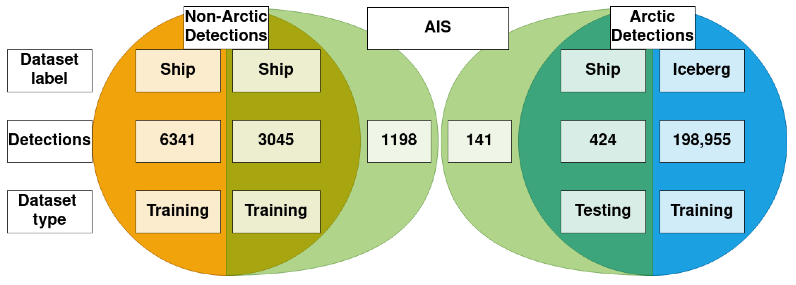
2. Data Acquisition
3. Methods for Ship and Iceberg Detection
3.1. Land Masking and Geocoding
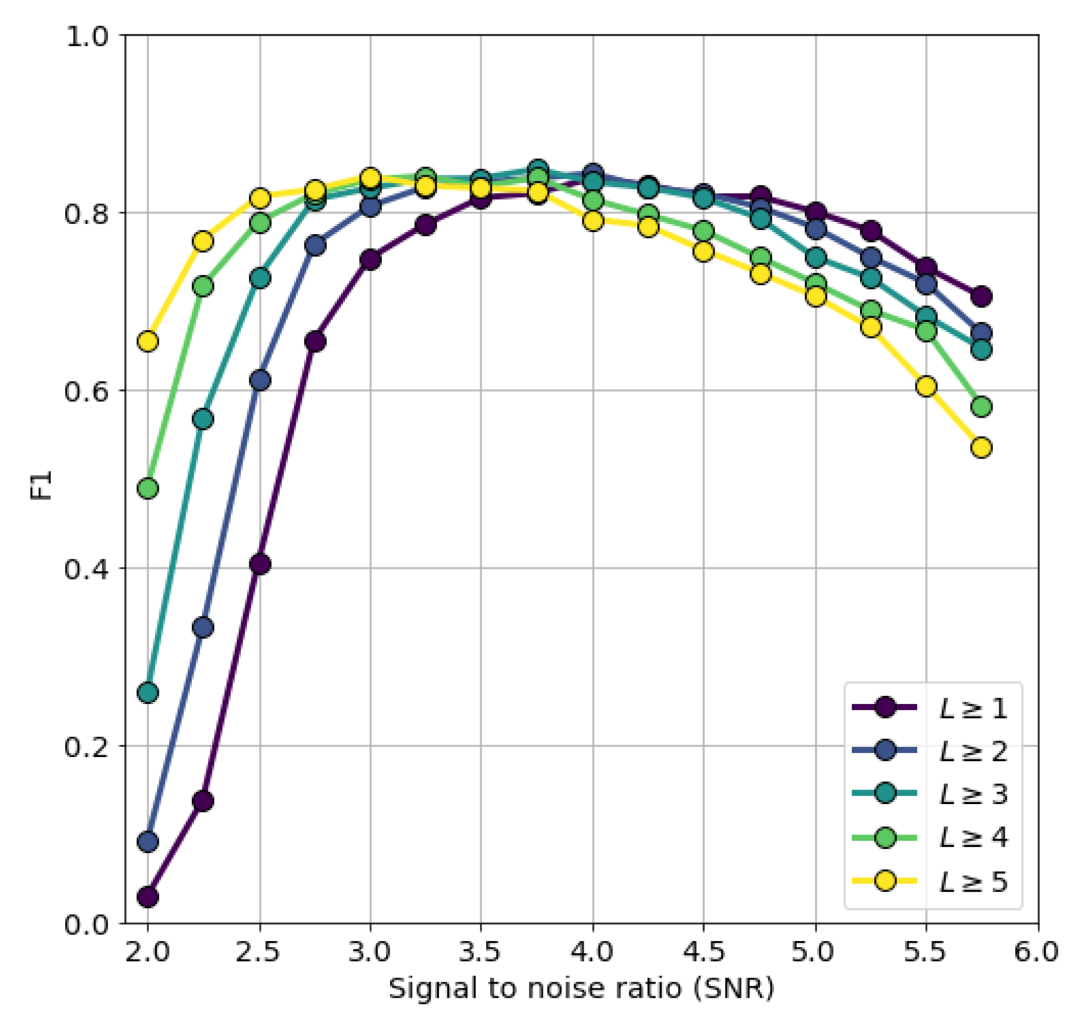
3.2. Detection Algorithm
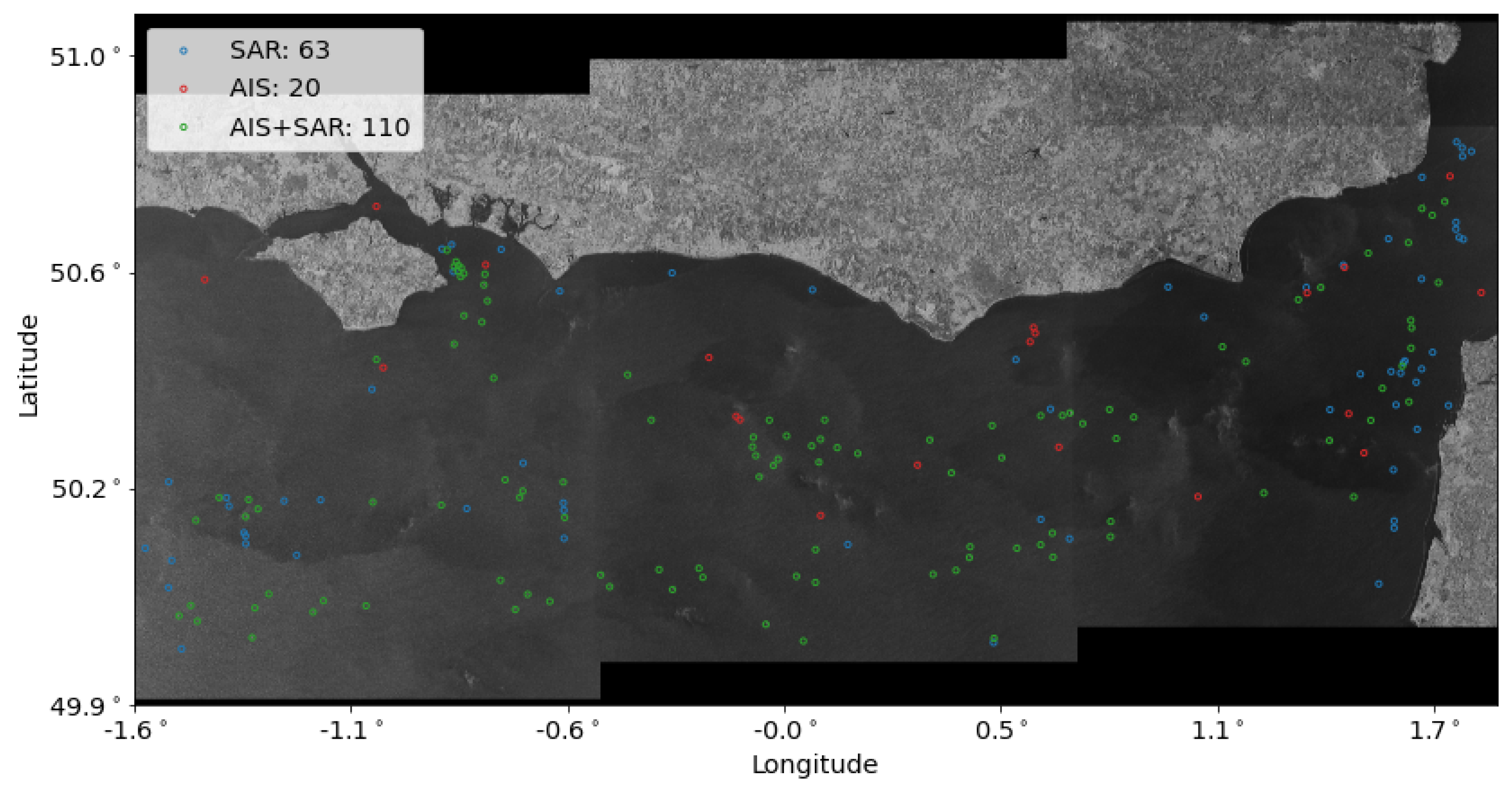
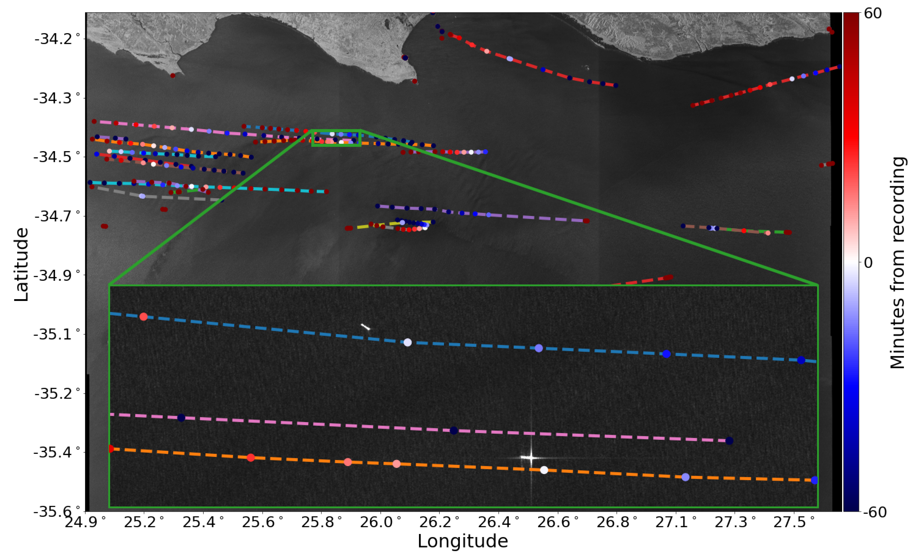
3.3. AIS-SAR Data Temporal and Spatial Association
3.4. Hyperparameter Selection
4. Methods for Ship–Iceberg Discrimination
4.1. Dataset
4.2. Convolutional Neural Networks
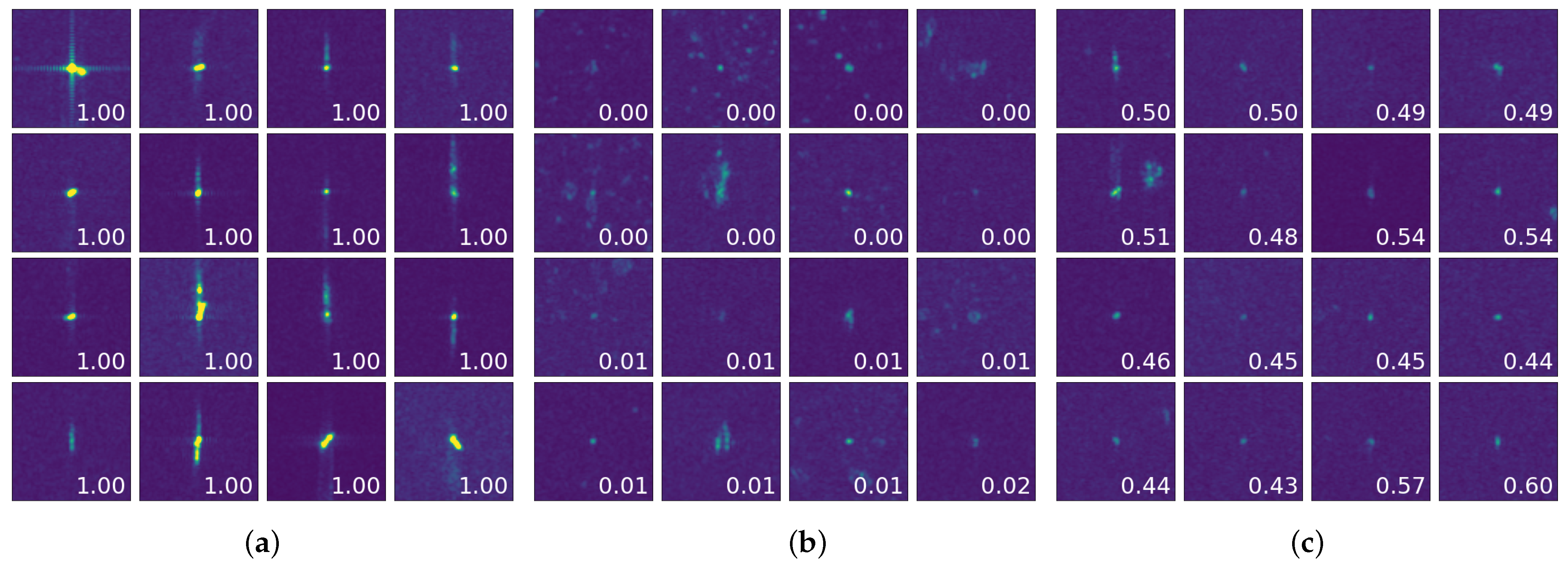
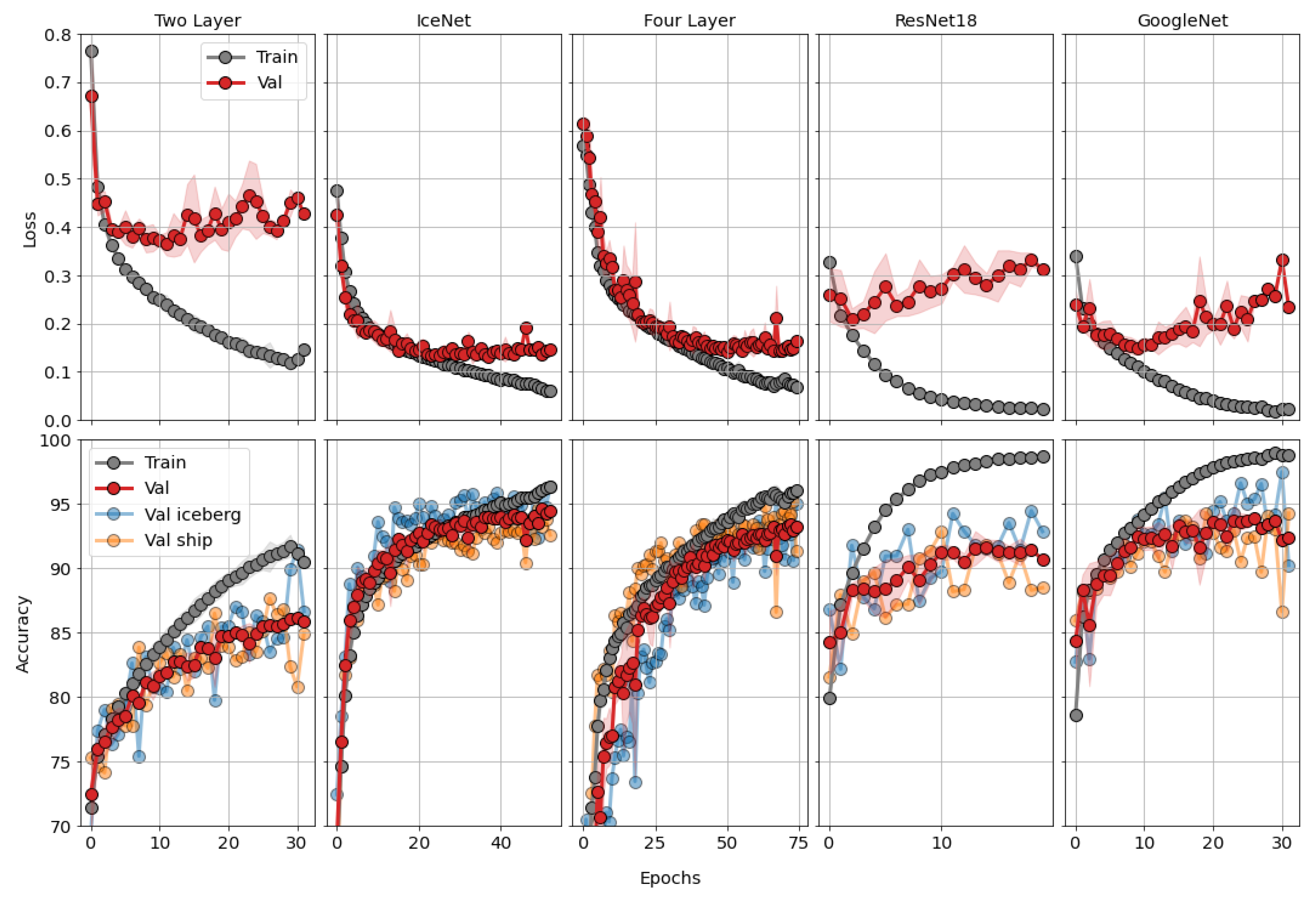
5. Results
6. Discussion
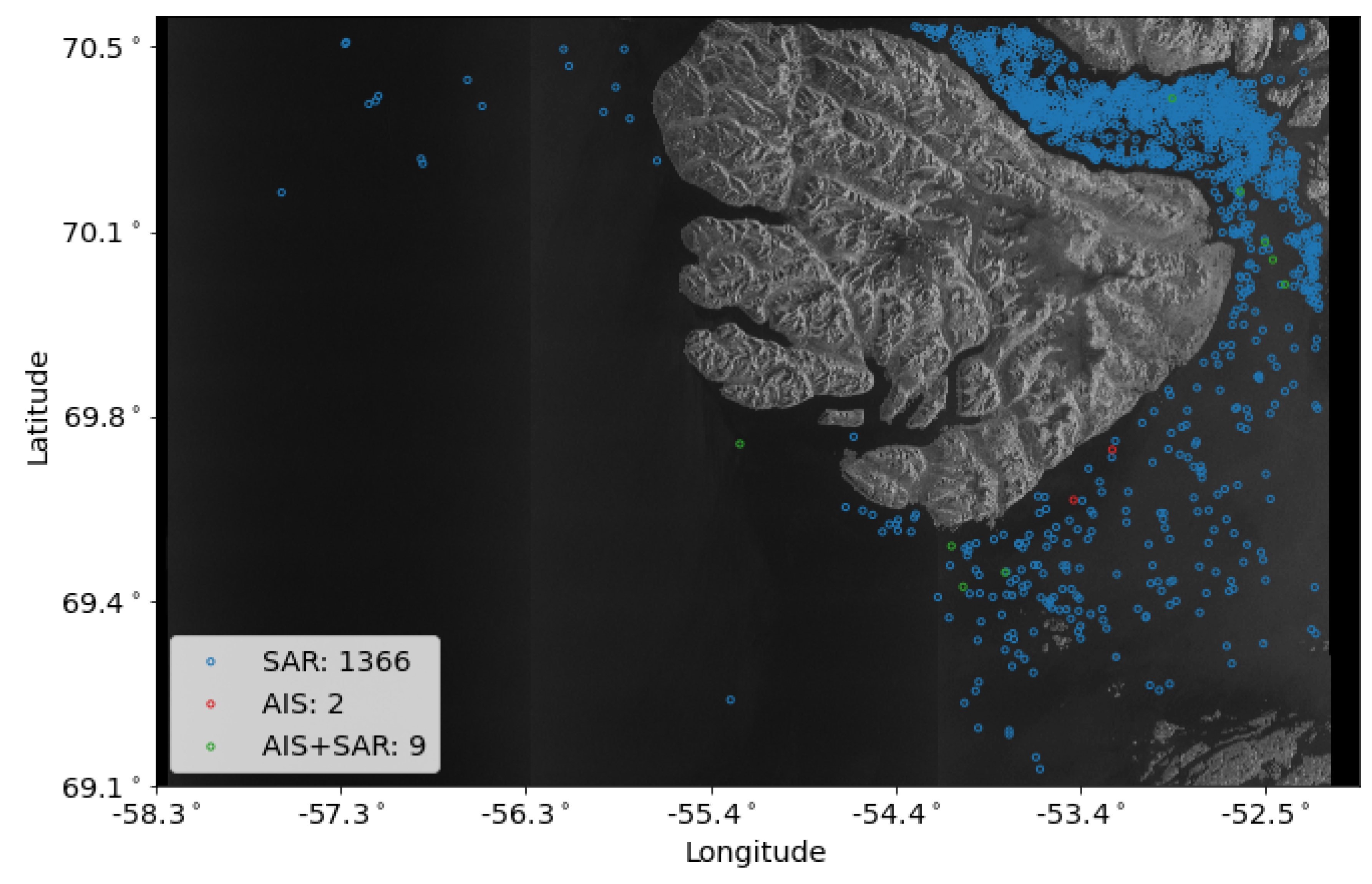
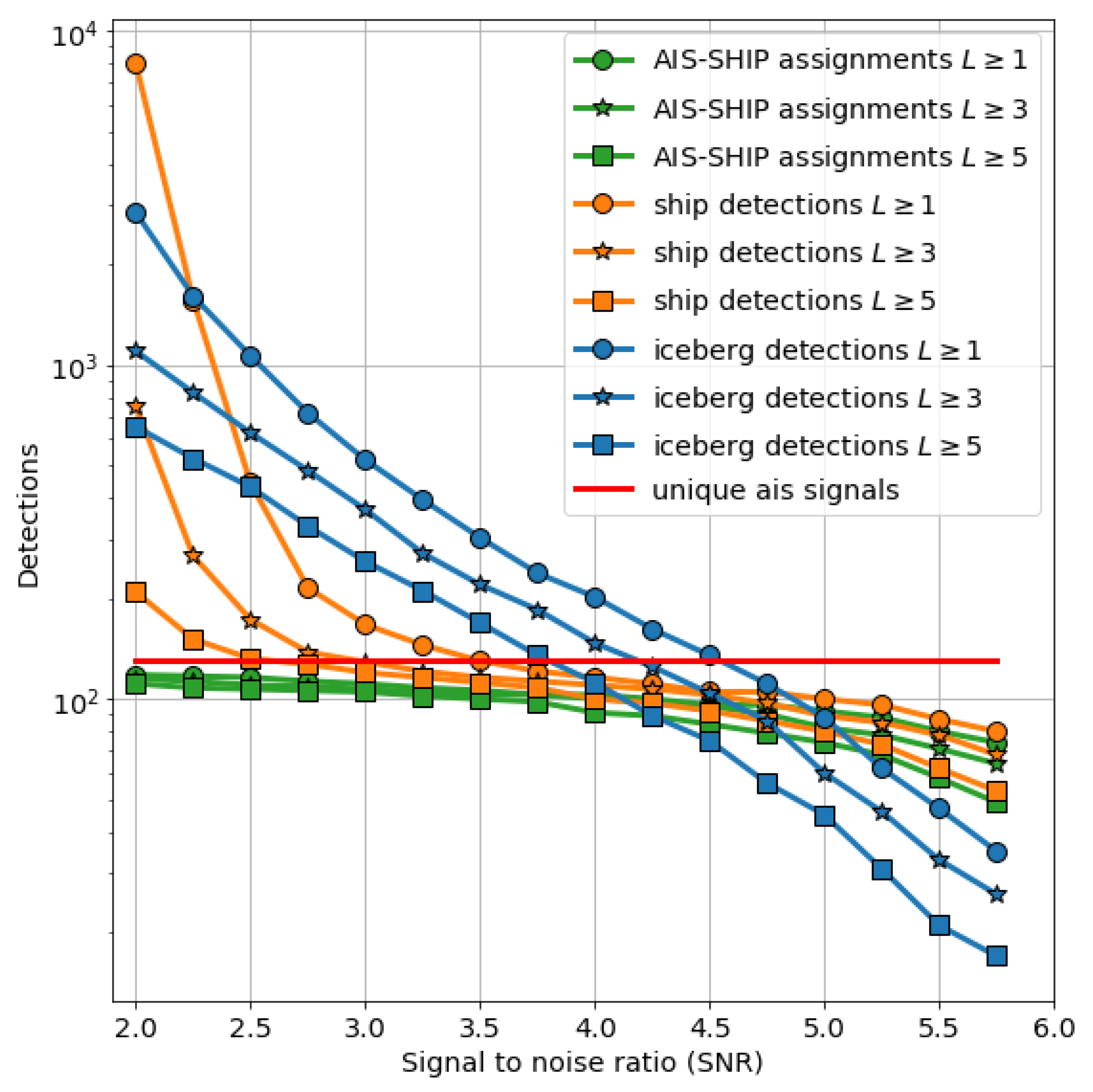
6.1. Detection of Ships and Icebergs, and AIS Correlation
6.2. Ship and Iceberg Discrimination
7. Conclusions
Author Contributions
Funding
Data Availability Statement
Acknowledgments
Conflicts of Interest
Abbreviations
| SAR | Synthetic Aperture Radar |
| AIS | Automatic Identification System |
| CNN | Convolutional Neural Network |
| CWT | Continuous Wavelet Transform |
| SNR | Signal to Noise Ratio |
| CFAR | Constant False Alarm Rate |
| ESA | European Space Agency |
References
- Barkham, P. Russian Tanker Sails through Arctic without Icebreaker for First Time. The Guardian, 24 August 2017. [Google Scholar]
- Chen, J.L.; Kang, S.C.; Guo, J.M.; Xu, M.; Zhang, Z.M. Variation of sea ice and perspectives of the Northwest Passage in the Arctic Ocean. Adv. Clim. Chang. Res. 2021, 12, 447–455. [Google Scholar] [CrossRef]
- Ball, H. Satellite AIS for Dummies; Wiley: Hoboken, NJ, USA, 2013. [Google Scholar]
- Høye, G.K.; Eriksen, T.; Meland, B.J.; Narheim, B.T. Space-based AIS for global maritime traffic monitoring. Acta Astronaut. 2008, 62, 240–245. [Google Scholar] [CrossRef]
- BBC. Warship Positions Faked Including UK Aircraft Carrier. BBC News, 2 August 2021. [Google Scholar]
- Crisp, D.J. The State-of-the-Art in Ship Detection in Synthetic Aperture Radar Imagery; Technical Report; Defence Science And Technology Organisation Salisbury (Australia). 2004. Available online: https://citeseerx.ist.psu.edu/viewdoc/download?doi=10.1.1.1000.6717&rep=rep1&type=pdf (accessed on 1 June 2021).
- Greidanus, H.; Alvarez, M.; Santamaria, C.; Thoorens, F.X.; Kourti, N.; Argentieri, P. The SUMO Ship Detector Algorithm for Satellite Radar Images. Remote Sens. 2017, 9, 246. [Google Scholar] [CrossRef] [Green Version]
- Palubinskas, G.; Reinartz, P.; Brusch, S.; Lehner, S. Joint Use of Optical and SAR Data for Ship Detection. 2009, pp. 1–6. Available online: https://elib.dlr.de (accessed on 1 June 2021).
- Yeremy, M.; Campbell, J.; Mattar, K.; Potter, T. Ocean Surveillance with Polarimetric SAR. Can. J. Remote Sens. 2001, 27, 328–344. [Google Scholar] [CrossRef]
- Touzi, R.; Charbonneau, F.J.; Hawkins, R.K.; Vachon, P.W. Ship detection and characterization using polarimetric SAR. Can. J. Remote Sens. 2004, 30, 552–559. [Google Scholar] [CrossRef]
- Touzi, R.; Charbonneau, F.; Hawkins, R.; Murnaghan, K.; Kavoun, X. Ship-sea contrast optimization when using polarimetric SARs. In Proceedings of the IGARSS 2001. Scanning the Present and Resolving the Future. Proceedings. IEEE 2001 International Geoscience and Remote Sensing Symposium (Cat. No.01CH37217), Sydney, Ausralia, 9–13 July 2001; Volume 1, pp. 426–428. [Google Scholar] [CrossRef]
- Sciotti, M.; Pastina, D.; Lombardo, P. Polarimetric detectors of extended targets for ship detection in SAR images. In Proceedings of the IGARSS 2001. Scanning the Present and Resolving the Future. Proceedings. IEEE 2001 International Geoscience and Remote Sensing Symposium (Cat. No.01CH37217), Sydney, Ausralia, 9–13 July 2001; Volume 7, pp. 3132–3134. [Google Scholar] [CrossRef]
- Sciotti, M.; Pastina, D.; Lombardo, P. Exploiting the polarimetric information for the detection of ship targets in non-homogeneous SAR images. In Proceedings of the IEEE International Geoscience and Remote Sensing Symposium, Toronto, ON, Canada, 24–28 June 2002; Volume 3, pp. 1911–1913. [Google Scholar] [CrossRef]
- Howell, C.; Youden, J.; Lane, K.; Power, D.; Randell, C.; Flett, D. Iceberg and ship discrimination with ENVISAT multipolarization ASAR. In Proceedings of the IGARSS 2004. 2004 IEEE International Geoscience and Remote Sensing Symposium, Anchorage, AL, USA, 20–24 September 2004; Volume 1, p. 116. [Google Scholar] [CrossRef]
- Howell, C.; Mills, J.; Power, D.; Youden, J.; Dodge, K.; Randell, C.; Churchill, S.; Flett, D. A multivariate approach to iceberg and ship classification in HH/HV ASAR data. In Proceedings of the 2006 IEEE International Symposium on Geoscience and Remote Sensing, Denver, CO, USA, 31 July–4 August 2006; pp. 3583–3586. [Google Scholar] [CrossRef]
- Heiselberg, P.; Heiselberg, H. Ship-Iceberg Discrimination in Sentinel-2 Multispectral Imagery by Supervised Classification. Remote Sens. 2017, 9, 1156. [Google Scholar] [CrossRef] [Green Version]
- Bentes, C.; Frost, A.; Velotto, D.; Tings, B. Ship-Iceberg Discrimination with Convolutional Neural Networks in High Resolution SAR Images. In Proceedings of the EUSAR 2016: 11th European Conference on Synthetic Aperture Radar, Hamburg, Germany, 6–9 June 2016; pp. 1–4. [Google Scholar]
- Statoil/C-CORE. Statoil/C-CORE Iceberg Classifier Challenge. 2018. Available online: https://www.kaggle.com/c/statoil-iceberg-classifier-challenge (accessed on 1 April 2021).
- Jang, H.; Kim, S.; Lam, T. Kaggle Competitions: Author Identification & Statoil/C-CORE Iceberg Classifier Challenge; Technical Report; School of Informatics, Computing, and Engineering, Indiana University: Bloomington, IN, USA, 2017. [Google Scholar]
- Yang, X.; Ding, J. A Computational Framework for Iceberg and Ship Discrimination: Case Study on Kaggle Competition. IEEE Access 2020, 8, 82320–82327. [Google Scholar] [CrossRef]
- Heiselberg, H. Ship-iceberg classification in SAR and multispectral satellite images with neural networks. Remote Sens. 2020, 12, 2353. [Google Scholar] [CrossRef]
- ESA Copernicus Program, Sentinel Scientific Data Hub. Available online: https://scihub.copernicus.eu/ (accessed on 1 October 2021).
- Zhang, T.; Zhang, X.; Ke, X.; Zhan, X.; Shi, J.; Wei, S.; Pan, D.; Li, J.; Su, H.; Zhou, Y.; et al. LS-SSDD-v1.0: A Deep Learning Dataset Dedicated to Small Ship Detection from Large-Scale Sentinel-1 SAR Images. Remote Sens. 2020, 12, 2997. [Google Scholar] [CrossRef]
- Alaska Satellite Facility (ASF) Distributed Active Archive Center. Available online: https://asf.alaska.edu/ (accessed on 1 October 2021).
- Wessel, P.; Smith, W.H. A global, self-consistent, hierarchical, high-resolution shoreline database. J. Geophys. Res. Solid Earth 1996, 101, 8741–8743. [Google Scholar] [CrossRef] [Green Version]
- Du, P.; Kibbe, W.A.; Lin, S.M. Improved peak detection in mass spectrum by incorporating continuous wavelet transform-based pattern matching. Bioinformatics 2006, 22, 2059–2065. [Google Scholar] [CrossRef] [PubMed] [Green Version]
- European Marine 140 Observation and Data Network (EMODnet). Available online: https://www.emodnet-humanactivities.eu/view-data.php (accessed on 14 March 2022).
- Sang, L.Z.; Yan, X.P.; Mao, Z.; Ma, F. Restoring method of vessel track based on AIS information. In Proceedings of the 2012 11th International Symposium on Distributed Computing and Applications to Business, Engineering & Science, Guilin, China, 19–22 October 2012; pp. 336–340. [Google Scholar]
- Rodger, M.; Guida, R. Classification-Aided SAR and AIS Data Fusion for Space-Based Maritime Surveillance. Remote Sens. 2020, 13, 104. [Google Scholar] [CrossRef]
- Heiselberg, H. Aircraft and Ship Velocity Determination in Sentinel-2 Multispectral Images. Sensors 2019, 19, 2873. [Google Scholar] [CrossRef] [PubMed] [Green Version]
- Szegedy, C.; Liu, W.; Jia, Y.; Sermanet, P.; Reed, S.E.; Anguelov, D.; Erhan, D.; Vanhoucke, V.; Rabinovich, A. Going Deeper with Convolutions. arXiv 2014, arXiv:1409.4842. [Google Scholar]
- Li, Y.; Ding, Z.; Zhang, C.; Wang, Y.; Chen, J. SAR ship detection based on resnet and transfer learning. In Proceedings of the 2019 IEEE International Geoscience and Remote Sensing Symposium (IGARSS 2019), Yokohama, Japan, 28 July–2 August 2019; pp. 1188–1191. [Google Scholar]
- Kang, K.M.; Kim, D.J. Ship velocity estimation from ship wakes detected using convolutional neural networks. IEEE J. Sel. Top. Appl. Earth Obs. Remote Sens. 2019, 12, 4379–4388. [Google Scholar] [CrossRef]
- He, K.; Zhang, X.; Ren, S.; Sun, J. Deep Residual Learning for Image Recognition. In Proceedings of the IEEE Conference on Computer Vision and Pattern Recognition, Boston, MA, USA, 7–12 June 2015. [Google Scholar]
- Marcel, S.; Rodriguez, Y. Torchvision the machine-vision package of torch. In Proceedings of the 18th ACM international conference on Multimedia, Firenze, Italy, 25–29 October 2010. [Google Scholar]
- Paszke, A.; Gross, S.; Massa, F.; Lerer, A.; Bradbury, J.; Chanan, G.; Killeen, T.; Lin, Z.; Gimelshein, N.; Antiga, L.; et al. PyTorch: An Imperative Style, High-Performance Deep Learning Library. In Advances in Neural Information Processing Systems 32 (NeurIPS 2019); Curran Associates, Inc.: Red Hook, NY, USA, 2019; Available online: http://papers.neurips.cc/paper/9015-pytorch-an-imperative-style-high-performance-deep-learning-library.pdf (accessed on 1 April 2021).
- Springenberg, J.T.; Dosovitskiy, A.; Brox, T.; Riedmiller, M. Striving for simplicity: The all convolutional net. arXiv 2014, arXiv:1412.6806. [Google Scholar]
- Srivastava, N.; Hinton, G.; Krizhevsky, A.; Sutskever, I.; Salakhutdinov, R. Dropout: A simple way to prevent neural networks from overfitting. J. Mach. Learn. Res. 2014, 15, 1929–1958. [Google Scholar]
- Ioffe, S.; Szegedy, C. Batch normalization: Accelerating deep network training by reducing internal covariate shift. In Proceedings of the International Conference on Machine Learning, Lille, France, 7–9 July 2015; pp. 448–456. [Google Scholar]
- Richards, M.A. Fundamentals of Radar Signal Processing; McGraw-Hill Education: New York, NY, USA, 2014. [Google Scholar]
- Nakkiran, P.; Kaplun, G.; Bansal, Y.; Yang, T.; Barak, B.; Sutskever, I. Deep double descent: Where bigger models and more data hurt. J. Stat. Mech. Theory Exp. 2021, 2021, 124003. [Google Scholar] [CrossRef]
- Heiselberg, H. Ship-iceberg detection & classification in sentinel-1 SAR images. TransNav 2020, 14, 235–241. [Google Scholar] [CrossRef]

| Model | Mean Loss | Mean Accuracy | Trainable Parameters |
|---|---|---|---|
| Two Layer | 16.417 | ||
| IceNet | 155.777 | ||
| Four Layer | 561.217 | ||
| ResNet18 | 5600.929 | ||
| GoogleNet | 11,177.025 |
| Dark Ships Included | AIS Only | |
|---|---|---|
| Ship accuracy | ||
| Iceberg accuracy | ||
| Ship PPV | ||
| Iceberg PPV |
Publisher’s Note: MDPI stays neutral with regard to jurisdictional claims in published maps and institutional affiliations. |
© 2022 by the authors. Licensee MDPI, Basel, Switzerland. This article is an open access article distributed under the terms and conditions of the Creative Commons Attribution (CC BY) license (https://creativecommons.org/licenses/by/4.0/).
Share and Cite
Heiselberg, P.; Sørensen, K.A.; Heiselberg, H.; Andersen, O.B. SAR Ship–Iceberg Discrimination in Arctic Conditions Using Deep Learning. Remote Sens. 2022, 14, 2236. https://doi.org/10.3390/rs14092236
Heiselberg P, Sørensen KA, Heiselberg H, Andersen OB. SAR Ship–Iceberg Discrimination in Arctic Conditions Using Deep Learning. Remote Sensing. 2022; 14(9):2236. https://doi.org/10.3390/rs14092236
Chicago/Turabian StyleHeiselberg, Peder, Kristian A. Sørensen, Henning Heiselberg, and Ole B. Andersen. 2022. "SAR Ship–Iceberg Discrimination in Arctic Conditions Using Deep Learning" Remote Sensing 14, no. 9: 2236. https://doi.org/10.3390/rs14092236
APA StyleHeiselberg, P., Sørensen, K. A., Heiselberg, H., & Andersen, O. B. (2022). SAR Ship–Iceberg Discrimination in Arctic Conditions Using Deep Learning. Remote Sensing, 14(9), 2236. https://doi.org/10.3390/rs14092236