
A Two-Branch Convolutional Neural Network Based on Multi-Spectral Entropy Rate Superpixel Segmentation for Hyperspectral Image Classification


Abstract
:1. Introduction
2. Materials and Methods
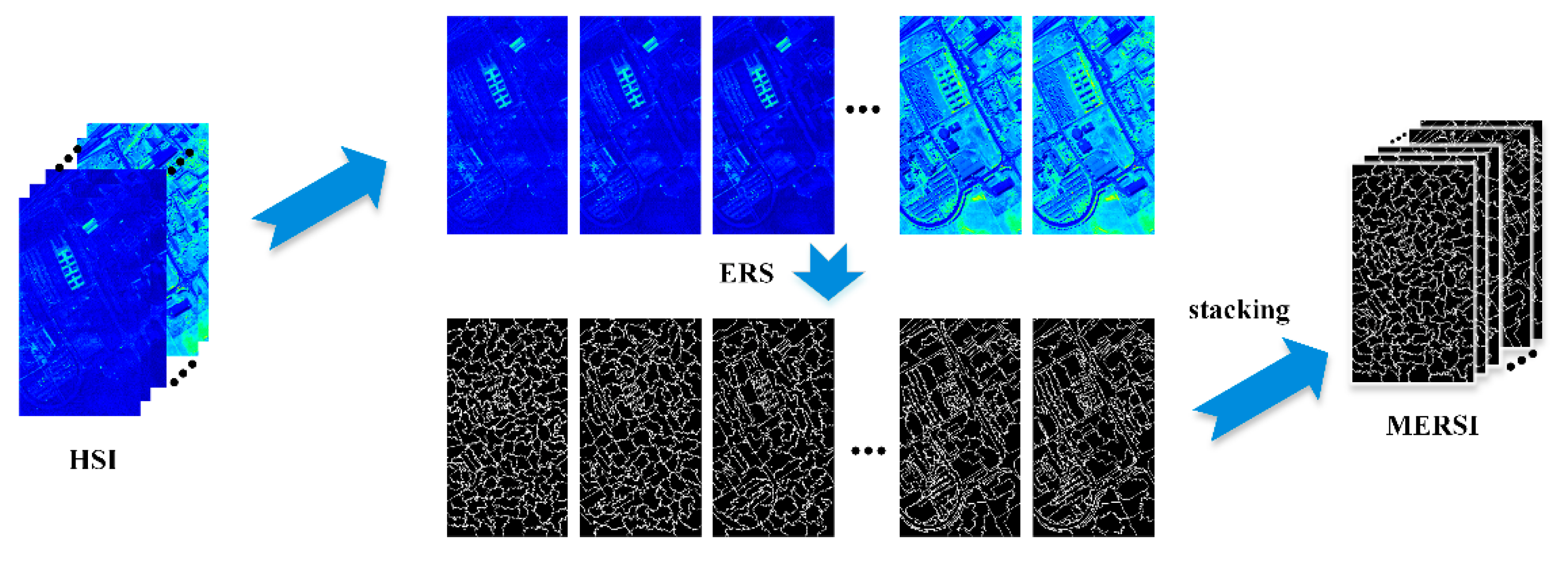
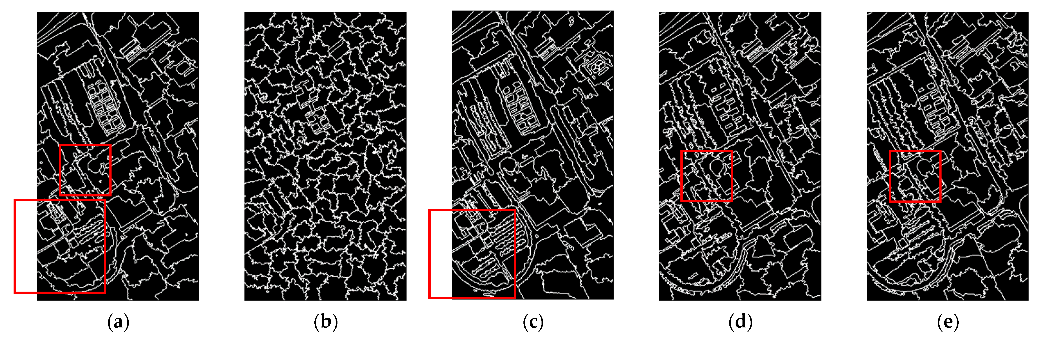
2.1. Multi-Spectral ERS
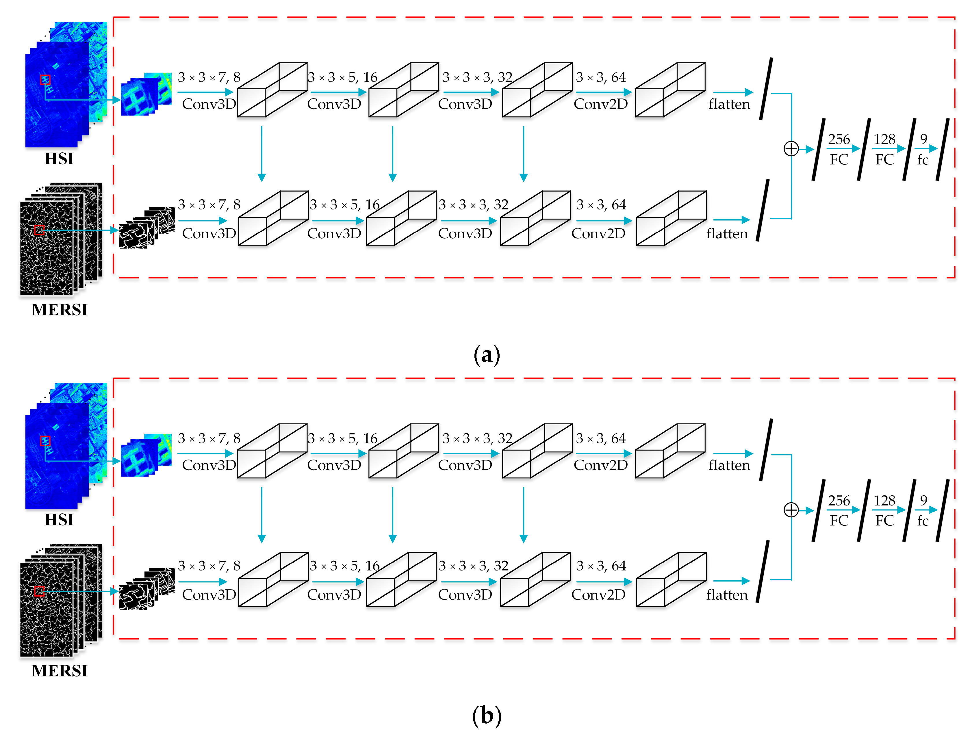
2.2. Two-Branch Convolutional Neural Network (TBN-MERS)
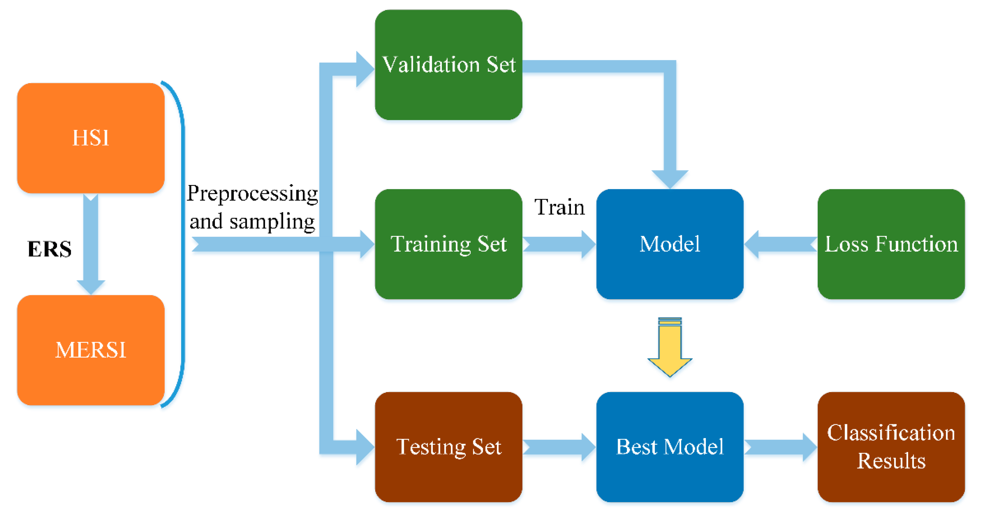
2.3. The Process of TBN-MERS
3. Results
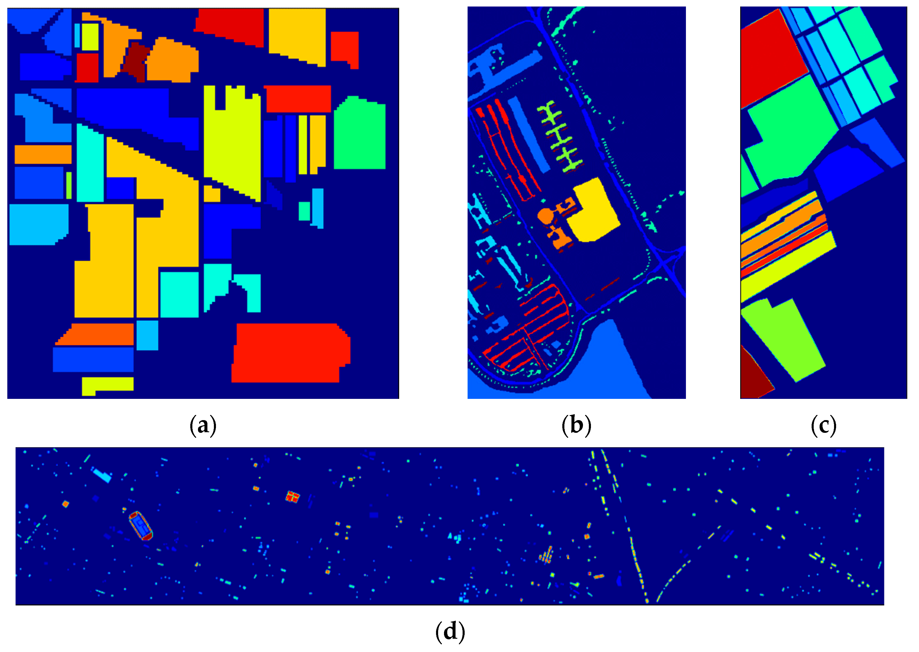
3.1. Datasets
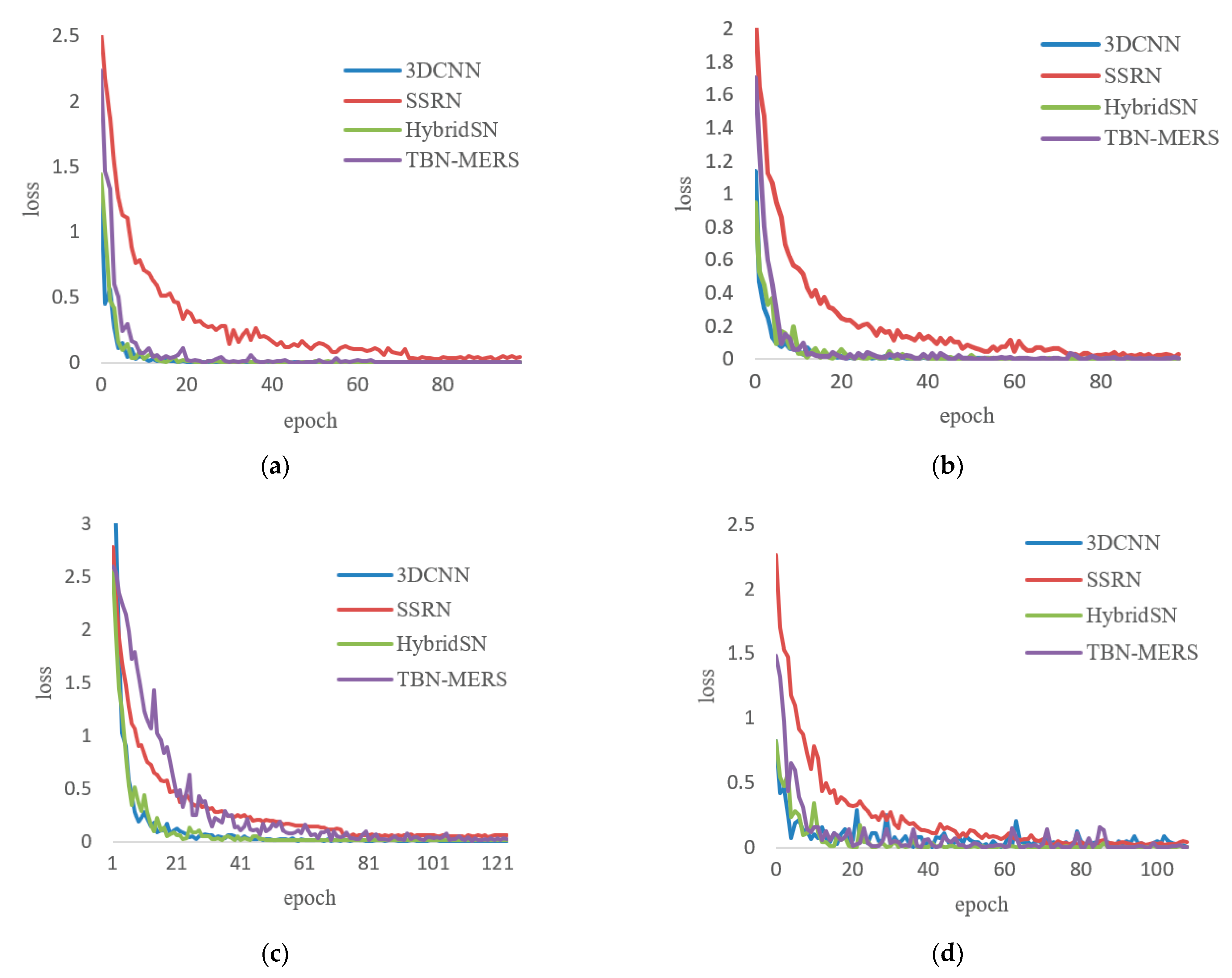
3.2. Experimental Settings
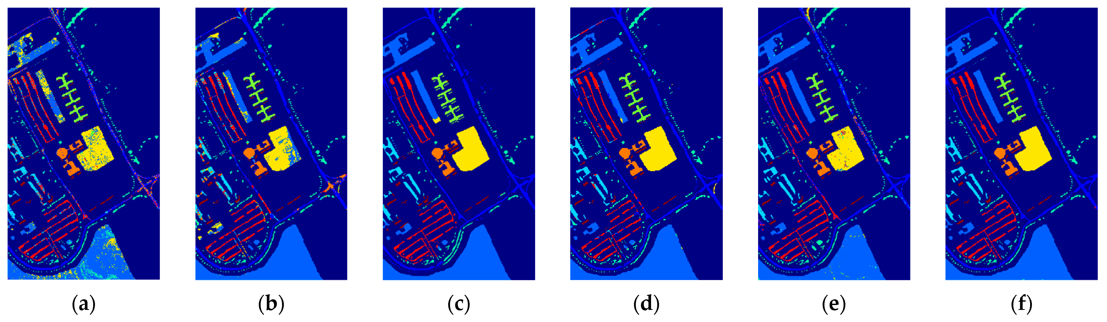
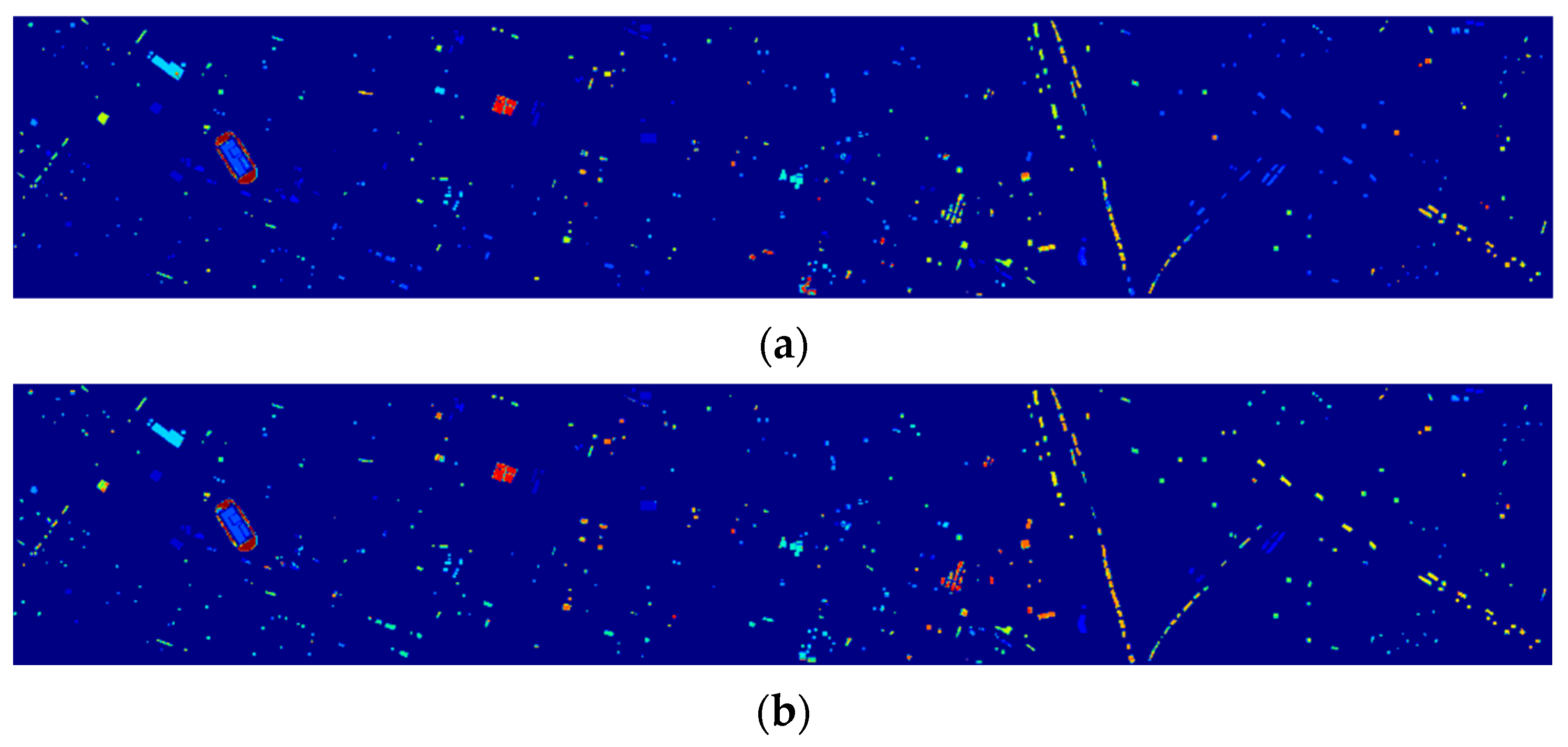
3.3. The Results and Analyses of Experiments
3.3.1. The Difference between Two-Branch Network and Single-Branch Network
3.3.2. The Influence of the Number of Superpixels and the Patch Size
3.3.3. The Difference of Multi-Spectral Methods Based on Two Kinds of Superpixel Segmentation Methods, ERS and SLIC
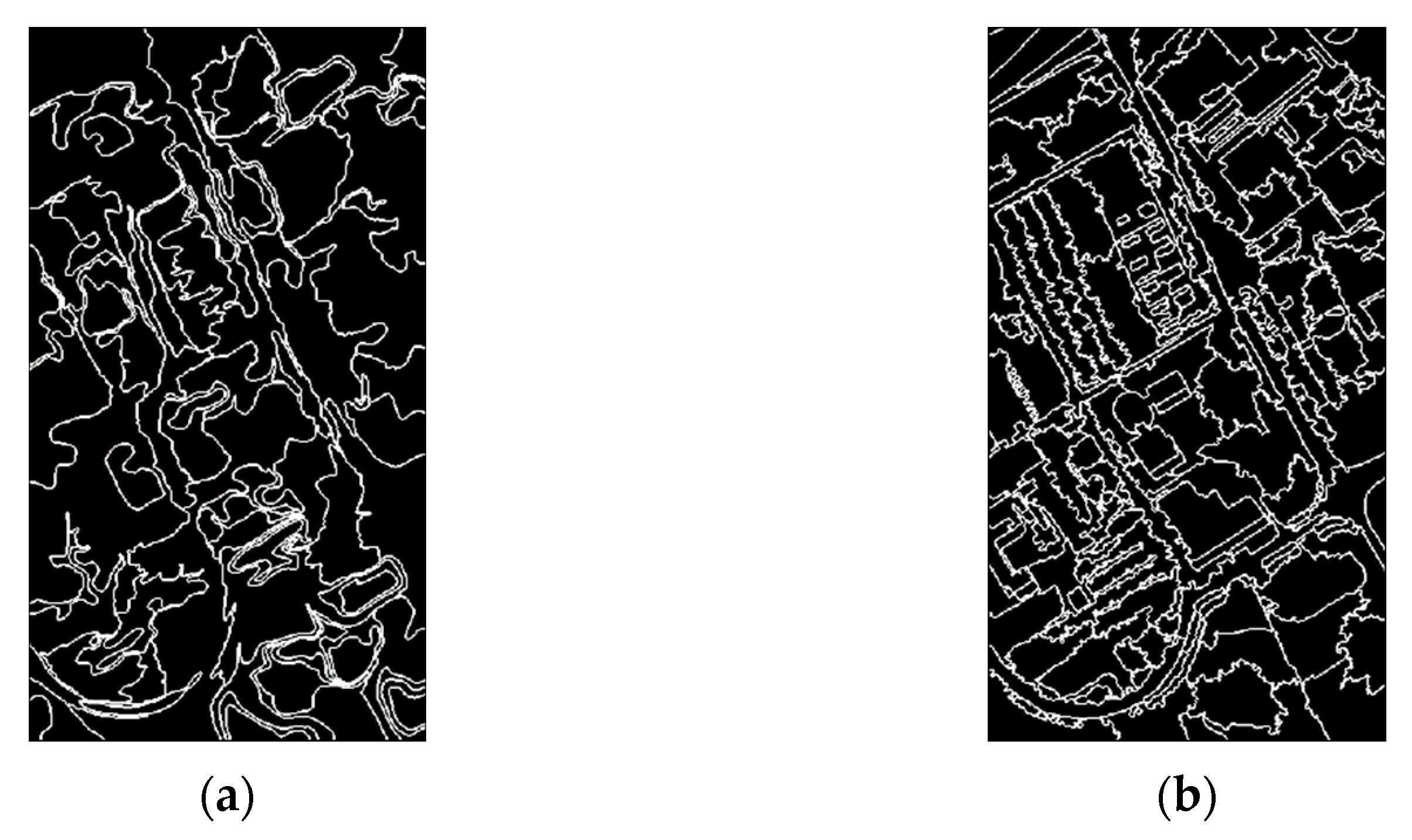
3.3.4. The Different Effects of Segmentation Images Obtained by Applying ERS to Images on Multiple Bands and the First Principal Component
3.3.5. The Effect of Using Different Fusion Methods in TBN-MERS
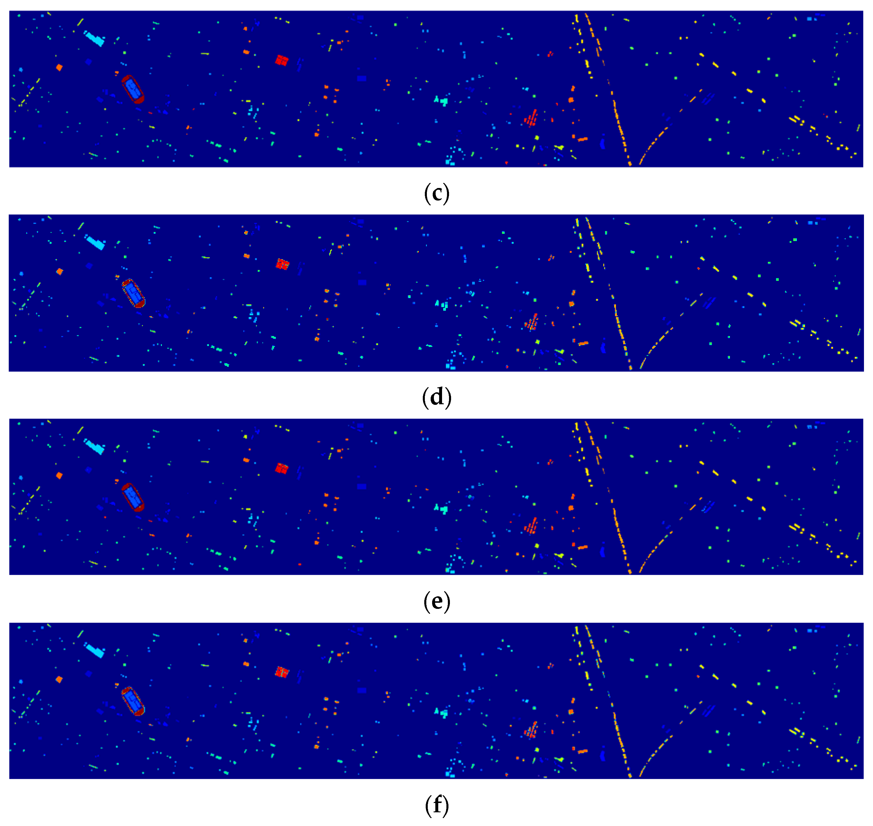
3.3.6. Comparison between TBN-MERS and Other Methods
4. Discussion
5. Conclusions
Author Contributions
Funding
Institutional Review Board Statement
Informed Consent Statement
Data Availability Statement
Acknowledgments
Conflicts of Interest
References
- Plaza, A.; Benediktsson, J.A.; Boardman, J.W.; Brazile, J.; Bruzzone, L.; Camps-Valls, G.; Chanussot, J.; Fauvel, M.; Gamba, P.; Gualtieri, A. Recent advances in techniques for hyperspectral image processing. Remote Sens. Environ. 2009, 113, S110–S122. [Google Scholar] [CrossRef]
- Hong, D.; Yokoya, N.; Chanussot, J.; Zhu, X.X. An augmented linear mixing model to address spectral variability for hyperspectral unmixing. IEEE Trans. Image Processing 2018, 28, 1923–1938. [Google Scholar] [CrossRef] [PubMed] [Green Version]
- Yao, J.; Meng, D.; Zhao, Q.; Cao, W.; Xu, Z. Nonconvex-sparsity and nonlocal-smoothness-based blind hyperspectral unmixing. IEEE Trans. Image Processing 2019, 28, 2991–3006. [Google Scholar] [CrossRef] [PubMed]
- Zhong, P.; Wang, R. Multiple-spectral-band CRFs for denoising junk bands of hyperspectral imagery. IEEE Trans. Geosci. Remote Sens. 2012, 51, 2260–2275. [Google Scholar] [CrossRef]
- Li, W.; Prasad, S.; Fowler, J.E.; Bruce, L.M. Locality-preserving dimensionality reduction and classification for hyperspectral image analysis. IEEE Trans. Geosci. Remote Sens. 2011, 50, 1185–1198. [Google Scholar] [CrossRef] [Green Version]
- Li, S.; Song, W.; Fang, L.; Chen, Y.; Ghamisi, P.; Benediktsson, J.A. Deep learning for hyperspectral image classification: An overview. IEEE Trans. Geosci. Remote Sens. 2019, 57, 6690–6709. [Google Scholar] [CrossRef] [Green Version]
- Camps-Valls, G.; Tuia, D.; Bruzzone, L.; Benediktsson, J.A. Advances in hyperspectral image classification: Earth monitoring with statistical learning methods. IEEE Signal Processing Mag. 2013, 31, 45–54. [Google Scholar] [CrossRef] [Green Version]
- Li, J.; Zhang, H.; Huang, Y.; Zhang, L. Hyperspectral image classification by nonlocal joint collaborative representation with a locally adaptive dictionary. IEEE Trans. Geosci. Remote Sens. 2013, 52, 3707–3719. [Google Scholar] [CrossRef]
- Plaza, A.; Martínez, P.; Plaza, J.; Pérez, R. Dimensionality reduction and classification of hyperspectral image data using sequences of extended morphological transformations. IEEE Trans. Geosci. Remote Sens. 2005, 43, 466–479. [Google Scholar] [CrossRef] [Green Version]
- Zhang, H.; Li, J.; Huang, Y.; Zhang, L. A nonlocal weighted joint sparse representation classification method for hyperspectral imagery. IEEE J. Sel. Top. Appl. Earth Obs. Remote Sens. 2013, 7, 2056–2065. [Google Scholar] [CrossRef]
- Cao, X.; Yao, J.; Xu, Z.; Meng, D. Hyperspectral image classification with convolutional neural network and active learning. IEEE Trans. Geosci. Remote Sens. 2020, 58, 4604–4616. [Google Scholar] [CrossRef]
- Chakrabarti, A.; Zickler, T. Statistics of real-world hyperspectral images. In Proceedings of the Conference on Computer Vision and Pattern Recognition (CVPR) 2011, Colorado Springs, CO, USA, 20–25 June 2011; pp. 193–200. [Google Scholar]
- Yasuma, F.; Mitsunaga, T.; Iso, D.; Nayar, S.K. Generalized assorted pixel camera: Postcapture control of resolution, dynamic range, and spectrum. IEEE Trans. Image Processing 2010, 19, 2241–2253. [Google Scholar] [CrossRef] [PubMed] [Green Version]
- Green, R.O.; Eastwood, M.L.; Sarture, C.M.; Chrien, T.G.; Aronsson, M.; Chippendale, B.J.; Faust, J.A.; Pavri, B.E.; Chovit, C.J.; Solis, M. Imaging spectroscopy and the airborne visible/infrared imaging spectrometer (AVIRIS). Remote Sens. Environ. 1998, 65, 227–248. [Google Scholar] [CrossRef]
- Bruzzone, L.; Cossu, R. A multiple-cascade-classifier system for a robust and partially unsupervised updating of land-cover maps. IEEE Trans. Geosci. Remote Sens. 2002, 40, 1984–1996. [Google Scholar] [CrossRef]
- Archibald, R.; Fann, G. Feature selection and classification of hyperspectral images with support vector machines. IEEE Geosci. Remote Sens. Lett. 2007, 4, 674–677. [Google Scholar] [CrossRef]
- Shao, Z.; Zhang, L.; Zhou, X.; Ding, L. A novel hierarchical semisupervised SVM for classification of hyperspectral images. IEEE Geosci. Remote Sens. Lett. 2014, 11, 1609–1613. [Google Scholar] [CrossRef]
- Chen, Y.; Nasrabadi, N.M.; Tran, T.D. Hyperspectral image classification via kernel sparse representation. IEEE Trans. Geosci. Remote Sens. 2012, 51, 217–231. [Google Scholar] [CrossRef] [Green Version]
- Chen, Y.; Lin, Z.; Zhao, X.; Wang, G.; Gu, Y. Deep learning-based classification of hyperspectral data. IEEE J. Sel. Top. Appl. Earth Obs. Remote Sens. 2014, 7, 2094–2107. [Google Scholar] [CrossRef]
- Chen, Y.; Zhao, X.; Jia, X. Spectral–spatial classification of hyperspectral data based on deep belief network. IEEE J. Sel. Top. Appl. Earth Obs. Remote Sens. 2015, 8, 2381–2392. [Google Scholar] [CrossRef]
- Hu, W.; Huang, Y.; Wei, L.; Zhang, F.; Li, H. Deep convolutional neural networks for hyperspectral image classification. J. Sens. 2015, 2015, 258619. [Google Scholar] [CrossRef] [Green Version]
- Yue, J.; Mao, S.; Li, M. A deep learning framework for hyperspectral image classification using spatial pyramid pooling. Remote Sens. Lett. 2016, 7, 875–884. [Google Scholar] [CrossRef]
- Cao, X.; Zhou, F.; Xu, L.; Meng, D.; Xu, Z.; Paisley, J. Hyperspectral image classification with Markov random fields and a convolutional neural network. IEEE Trans. Image Processing 2018, 27, 2354–2367. [Google Scholar] [CrossRef] [PubMed] [Green Version]
- Hamida, A.B.; Benoit, A.; Lambert, P.; Amar, C.B. 3-D deep learning approach for remote sensing image classification. IEEE Trans. Geosci. Remote Sens. 2018, 56, 4420–4434. [Google Scholar] [CrossRef] [Green Version]
- Zhong, Z.; Li, J.; Luo, Z.; Chapman, M. Spectral–spatial residual network for hyperspectral image classification: A 3-D deep learning framework. IEEE Trans. Geosci. Remote Sens. 2017, 56, 847–858. [Google Scholar] [CrossRef]
- Roy, S.K.; Krishna, G.; Dubey, S.R.; Chaudhuri, B.B. HybridSN: Exploring 3-D–2-D CNN feature hierarchy for hyperspectral image classification. IEEE Geosci. Remote Sens. Lett. 2019, 17, 277–281. [Google Scholar] [CrossRef] [Green Version]
- Leng, Q.; Yang, H.; Jiang, J.; Tian, Q. Adaptive multiscale segmentations for hyperspectral image classification. IEEE Trans. Geosci. Remote Sens. 2020, 58, 5847–5860. [Google Scholar] [CrossRef]
- Jiang, J.; Ma, J.; Chen, C.; Wang, Z.; Cai, Z.; Wang, L. SuperPCA: A superpixelwise PCA approach for unsupervised feature extraction of hyperspectral imagery. IEEE Trans. Geosci. Remote Sens. 2018, 56, 4581–4593. [Google Scholar] [CrossRef] [Green Version]
- Mei, X.; Pan, E.; Ma, Y.; Dai, X.; Huang, J.; Fan, F.; Du, Q.; Zheng, H.; Ma, J. Spectral-spatial attention networks for hyperspectral image classification. Remote Sens. 2019, 11, 963. [Google Scholar] [CrossRef] [Green Version]
- Mu, C.; Zeng, Q.; Liu, Y.; Qu, Y. A two-branch network combined with robust principal component analysis for hyperspectral image classification. IEEE Geosci. Remote Sens. Lett. 2020, 18, 2147–2151. [Google Scholar] [CrossRef]
- Varga, D. Composition-preserving deep approach to full-reference image quality assessment. Signal Image Video Processing 2020, 14, 1265–1272. [Google Scholar] [CrossRef]
- Saenz, H.; Sun, H.; Wu, L.; Zhou, X.; Yu, H. Detecting phone-related pedestrian distracted behaviours via a two-branch convolutional neural network. IET Intell. Transp. Syst. 2021, 15, 147–158. [Google Scholar] [CrossRef]
- Mori, G.; Ren, X.; Efros, A.A.; Malik, J. Recovering human body configurations: Combining segmentation and recognition. In Proceedings of the 2004 IEEE Computer Society Conference on Computer Vision and Pattern Recognition (CVPR), Washington, DC, USA, 27 June–2 July 2004; p. II. [Google Scholar]
- Ren, X.; Malik, J. Learning a classification model for segmentation. In Proceedings of the Proceedings Ninth IEEE International Conference on Computer VisionComputer Vision, Nice, France, 13–16 October 2003; p. 10. [Google Scholar]
- Kohli, P.; Torr, P.H. Robust higher order potentials for enforcing label consistency. Int. J. Comput. Vis. 2009, 82, 302–324. [Google Scholar] [CrossRef] [Green Version]
- Achanta, R.; Shaji, A.; Smith, K.; Lucchi, A.; Fua, P.; Süsstrunk, S. SLIC superpixels compared to state-of-the-art superpixel methods. IEEE Trans. Pattern Anal. Mach. Intell. 2012, 34, 2274–2282. [Google Scholar] [CrossRef] [PubMed] [Green Version]
- Liu, M.; Tuzel, O.; Ramalingam, S.; Chellappa, R. Entropy rate superpixel segmentation. In Proceedings of the Conference on Computer Vision and Pattern Recognition (CVPR) 2011, Colorado Springs, CO, USA, 20–25 June 2011; pp. 2097–2104. [Google Scholar]
- Comaniciu, D.; Meer, P. Mean shift: A robust approach toward feature space analysis. IEEE Trans. Pattern Anal. Mach. Intell. 2002, 24, 603–619. [Google Scholar] [CrossRef] [Green Version]
- Vincent, L.; Soille, P. Watersheds in digital spaces: An efficient algorithm based on immersion simulations. IEEE Trans. Pattern Anal. Mach. Intell. 1991, 13, 583–598. [Google Scholar] [CrossRef] [Green Version]
- Shi, J.; Malik, J. Normalized cuts and image segmentation. IEEE Trans. Pattern Anal. Mach. Intell. 2000, 22, 888–905. [Google Scholar]
- Felzenszwalb, P.F.; Huttenlocher, D.P. Efficient graph-based image segmentation. Int. J. Comput. Vis. 2004, 59, 167–181. [Google Scholar] [CrossRef]
- Levinshtein, A.; Stere, A.; Kutulakos, K.N.; Fleet, D.J.; Dickinson, S.J.; Siddiqi, K. Turbopixels: Fast superpixels using geometric flows. IEEE Trans. Pattern Anal. Mach. Intell. 2009, 31, 2290–2297. [Google Scholar] [CrossRef] [Green Version]
- Veksler, O.; Boykov, Y.; Mehrani, P. Superpixels and supervoxels in an energy optimization framework. In Proceedings of the European Conference on Computer Vision, Heraklion, Greece, 5–11 September 2010; pp. 211–224. [Google Scholar]


| Layers | Kernel Size | Number of Kernels | Padding |
|---|---|---|---|
| Cov3D_1 | (3,3,7) | 8 | 1 |
| Cov3D_2 | (3,3,5) | 16 | 1 |
| Cov3D_3 | (3,3,3) | 32 | 1 |
| Cov2D | (3,3) | 64 | 1 |
| FC_1 | -- | 256 | -- |
| FC_2 | -- | 128 | -- |
| fc | -- | Number of classes | -- |
| Number | Class | Samples | Color |
|---|---|---|---|
| 1 | Alfalfa | 46 | |
| 2 | Corn-notill | 1428 | |
| 3 | Corn-mintill | 830 | |
| 4 | Corn | 237 | |
| 5 | Grass-pasture | 483 | |
| 6 | Grass-trees | 730 | |
| 7 | Grass-pasture-mowed | 28 | |
| 8 | Hay-windrowed | 478 | |
| 9 | Oats | 20 | |
| 10 | Soybean-notill | 972 | |
| 11 | Soybean-mintill | 2455 | |
| 12 | Soybean-clean | 593 | |
| 13 | Wheat | 205 | |
| 14 | Woods | 1265 | |
| 15 | Buildings-Grass-Trees-Drives | 386 | |
| 16 | Stone-Steel-Towers | 93 | |
| Total | 10,249 |
| Number | Class | Samples | Color |
|---|---|---|---|
| 1 | Asphalt | 6631 | |
| 2 | Meadows | 18,649 | |
| 3 | Gravel | 2099 | |
| 4 | Trees | 3064 | |
| 5 | Painted metal sheets | 1345 | |
| 6 | Bare Soil | 5029 | |
| 7 | Bitumen | 1330 | |
| 8 | Self-Blocking Bricks | 3682 | |
| 9 | Shadows | 947 | |
| Total | 42,776 |
| Number | Class | Samples | Color |
|---|---|---|---|
| 1 | Brocoli_green_weeds_1 | 2009 | |
| 2 | Brocoli_green_weeds_2 | 3726 | |
| 3 | Fallow | 1976 | |
| 4 | Fallow_rough_plow | 1394 | |
| 5 | Fallow_smooth | 2678 | |
| 6 | Stubble | 3959 | |
| 7 | Celery | 3579 | |
| 8 | Grapes_untrained | 11,271 | |
| 9 | Soil_vinyard_develop | 6203 | |
| 10 | Corn_senesced_green_weeds | 3278 | |
| 11 | Lettuce_romaine_4wk | 1068 | |
| 12 | Lettuce_romaine_5wk | 1927 | |
| 13 | Lettuce_romaine_6wk | 916 | |
| 14 | Lettuce_romaine_7wk | 1070 | |
| 15 | Vinyard_untrained | 7268 | |
| 16 | Vinyard_vertical_trellis | 1807 | |
| Total | 54,129 |
| Number | Class | Samples | Color |
|---|---|---|---|
| 1 | Healthy grass | 1251 | |
| 2 | Stressed grass | 1254 | |
| 3 | Synthetic grass | 732 | |
| 4 | Trees | 1244 | |
| 5 | Soil | 1242 | |
| 6 | Water | 339 | |
| 7 | Residential | 1268 | |
| 8 | Commercial | 1244 | |
| 9 | Road | 1252 | |
| 10 | Highway | 1227 | |
| 11 | Railway | 1288 | |
| 12 | Parking Lot 1 | 1233 | |
| 13 | Parking Lot 2 | 531 | |
| 14 | Tennis Court | 463 | |
| 15 | Running Track | 700 | |
| Total | 15,268 |
| Networks | Metrics | IP | PU | SA | HU |
|---|---|---|---|---|---|
| Net-X | OA (%) | 81.02 | 94.63 | 85.31 | 94.68 |
| AA (%) | 87.70 | 94.33 | 91.74 | 95.39 | |
| Kappa (×100) | 78.44 | 92.88 | 83.59 | 94.25 | |
| Net-S | OA (%) | 97.59 | 95.90 | 97.89 | 90.58 |
| AA (%) | 98.97 | 96.37 | 98.65 | 91.90 | |
| Kappa (×100) | 97.23 | 94.58 | 97.66 | 89.83 | |
| TBN-MERS | OA (%) | 98.13 | 99.74 | 99.35 | 97.51 |
| AA (%) | 99.01 | 99.70 | 99.31 | 97.88 | |
| Kappa (×100) | 97.85 | 99.66 | 99.28 | 97.31 |
| Methods | Metrics | IP | PU | SA | HU |
|---|---|---|---|---|---|
| TBN-MSLIC | OA (%) | 95.01 | 99.20 | 95.16 | 96.59 |
| AA (%) | 97.48 | 99.55 | 96.55 | 97.13 | |
| Kappa (×100) | 94.28 | 98.94 | 94.62 | 96.31 | |
| TBN-MERS | OA (%) | 98.13 | 99.74 | 99.35 | 97.51 |
| AA (%) | 99.01 | 99.70 | 99.31 | 97.88 | |
| Kappa (×100) | 97.85 | 99.66 | 99.28 | 97.31 |
| Methods | Metrics | IP | PU | SA | HU |
|---|---|---|---|---|---|
| PC-TBN-MERS | OA (%) | 86.58 | 97.80 | 93.79 | 96.28 |
| AA (%) | 91.91 | 97.78 | 95.40 | 96.68 | |
| Kappa (×100) | 84.72 | 97.08 | 93.10 | 95.98 | |
| TBN-MERS | OA (%) | 98.13 | 99.74 | 99.35 | 97.51 |
| AA (%) | 99.01 | 99.70 | 99.31 | 97.88 | |
| Kappa (×100) | 97.85 | 99.66 | 99.28 | 97.31 |
| Methods | Metrics | IP | PU | SA | HU |
|---|---|---|---|---|---|
| TBN(M2H)-MERS | OA (%) | 97.74 | 97.74 | 99.12 | 94.81 |
| AA (%) | 98.99 | 98.29 | 98.94 | 95.72 | |
| Kappa (×100) | 97.41 | 97.01 | 99.02 | 94.39 | |
| TBN(H2M)-MERS | OA (%) | 93.62 | 98.94 | 97.34 | 96.34 |
| AA (%) | 96.41 | 99.30 | 97.14 | 96.87 | |
| Kappa (×100) | 92.70 | 98.60 | 97.04 | 96.05 | |
| TBN-MERS | OA (%) | 98.13 | 99.74 | 99.35 | 97.51 |
| AA (%) | 99.01 | 99.70 | 99.31 | 97.88 | |
| Kappa (×100) | 97.85 | 99.66 | 99.28 | 97.31 |
| Class Number | SVM [16] | 3DCNN [24] | SSRN [25] | HybridSN [26] | SuperPCA [28] | TBN-MERS |
|---|---|---|---|---|---|---|
| 1 | 66.11 | 99.37 | 0.00 | 100.00 | 100.00 | 100.00 |
| 2 | 63.91 | 78.03 | 76.71 | 87.80 | 93.76 | 98.21 |
| 3 | 64.17 | 70.64 | 86.27 | 96.76 | 89.10 | 94.64 |
| 4 | 84.38 | 61.16 | 100.00 | 99.35 | 95.19 | 100.00 |
| 5 | 90.71 | 88.95 | 94.67 | 97.50 | 97.00 | 98.33 |
| 6 | 92.79 | 93.52 | 97.41 | 96.91 | 95.29 | 99.94 |
| 7 | 85.55 | 98.88 | 0.00 | 100.00 | 85.71 | 100.00 |
| 8 | 95.23 | 97.60 | 100.00 | 100.00 | 99.53 | 100.00 |
| 9 | 88.00 | 94.84 | 0.00 | 100.00 | 90.00 | 100.00 |
| 10 | 72.14 | 64.13 | 88.21 | 93.55 | 81.13 | 97.22 |
| 11 | 57.04 | 90.11 | 87.31 | 89.47 | 85.07 | 96.92 |
| 12 | 70.01 | 73.23 | 74.11 | 94.91 | 93.74 | 98.96 |
| 13 | 98.58 | 91.95 | 99.31 | 100.00 | 99.35 | 100.00 |
| 14 | 83.09 | 94.71 | 98.01 | 97.99 | 97.20 | 100.00 |
| 15 | 70.47 | 77.04 | 99.94 | 97.91 | 98.81 | 100.00 |
| 16 | 97.67 | 77.40 | 99.05 | 100.00 | 97.83 | 100.00 |
| OA (%) | 71.86 (0.34) | 82.16 (1.47) | 88.38 (1.58) | 93.77 (1.22) | 95.06 (1.24) | 98.13 (0.21) |
| AA (%) | 79.99 (0.93) | 84.47 (1.58) | 75.06 (1.07) | 97.01 (0.55) | 96.70 (1.00) | 99.01 (0.09) |
| Kappa (×100) | 68.22 (0.41) | 79.72 (1.65) | 86.73 (1.79) | 92.88 (1.38) | 94.32 (1.42) | 97.85 (0.24) |
| Class Number | SVM [16] | 3DCNN [24] | SSRN [25] | HybridSN [26] | SuperPCA [28] | TBN-MERS |
|---|---|---|---|---|---|---|
| 1 | 77.34 | 95.27 | 92.55 | 87.33 | 70.66 | 99.74 |
| 2 | 80.62 | 94.78 | 98.40 | 98.38 | 80.93 | 99.89 |
| 3 | 79.59 | 66.67 | 97.62 | 94.74 | 93.70 | 99.50 |
| 4 | 95.08 | 93.30 | 70.38 | 94.10 | 80.23 | 98.95 |
| 5 | 99.32 | 99.42 | 99.67 | 99.84 | 96.60 | 100.00 |
| 6 | 79.97 | 75.00 | 99.75 | 99.86 | 87.73 | 100.00 |
| 7 | 93.06 | 63.18 | 97.51 | 99.93 | 92.97 | 100.00 |
| 8 | 84.86 | 84.21 | 99.38 | 89.00 | 91.88 | 99.53 |
| 9 | 99.86 | 96.08 | 68.34 | 93.73 | 100.00 | 100.00 |
| OA (%) | 82.73 (1.78) | 88.38 (0.99) | 95.08 (1.27) | 95.54 (0.71) | 93.24 (0.67) | 99.86 (0.07) |
| AA (%) | 87.75 (0.42) | 85.32 (0.94) | 91.51 (1.00) | 95.21 (0.70) | 94.42 (0.37) | 99.77 (0.08) |
| Kappa (×100) | 77.78 (2.08) | 84.69 (1.25) | 93.47 (1.66) | 94.09 (0.94) | 91.10 (0.85) | 99.64 (0.09) |
| Class Number | SVM [16] | 3DCNN [24] | SSRN [25] | HybridSN [26] | SuperPCA [28] | TBN-MERS |
|---|---|---|---|---|---|---|
| 1 | 98.35 | 73.44 | 99.67 | 98.65 | 100.00 | 100.00 |
| 2 | 81.50 | 97.13 | 95.17 | 97.32 | 73.53 | 100.00 |
| 3 | 37.44 | 99.48 | 96.14 | 97.54 | 87.27 | 100.00 |
| 4 | 97.99 | 98.52 | 93.80 | 83.94 | 70.27 | 99.98 |
| 5 | 93.92 | 99.48 | 80.07 | 91.73 | 51.63 | 97.23 |
| 6 | 97.20 | 99.96 | 99.09 | 97.92 | 85.31 | 99.39 |
| 7 | 99.02 | 91.03 | 92.90 | 99.25 | 72.97 | 100.00 |
| 8 | 37.31 | 66.54 | 71.32 | 85.45 | 33.37 | 98.95 |
| 9 | 97.97 | 86.99 | 100.00 | 94.20 | 53.34 | 99.93 |
| 10 | 24.32 | 86.16 | 82.38 | 91.03 | 66.27 | 98.75 |
| 11 | 83.55 | 95.99 | 73.93 | 94.93 | 96.33 | 99.34 |
| 12 | 96.13 | 93.55 | 62.59 | 97.00 | 78.15 | 99.76 |
| 13 | 98.77 | 89.27 | 49.98 | 96.11 | 95.28 | 99.62 |
| 14 | 88.45 | 85.89 | 94.70 | 99.26 | 71.74 | 98.74 |
| 15 | 57.51 | 59.00 | 52.28 | 75.95 | 100.00 | 99.59 |
| 16 | 71.67 | 98.78 | 77.88 | 97.67 | 74.97 | 97.03 |
| OA (%) | 70.52 (1.19) | 82.47 (0.83) | 80.85 (4.37) | 90.82 (1.89) | 73.64 (3.53) | 99.31 (0.13) |
| AA (%) | 78.82 (0.81) | 88.83 (1.01) | 82.62 (5.78) | 93.62 (0.89) | 81.35 (2.46) | 99.27 (0.13) |
| Kappa (×100) | 67.37 (1.29) | 80.39 (0.92) | 78.71 (4.88) | 89.78 (2.12) | 70.92 (3.65) | 99.23 (0.15) |
| Class Number | SVM [16] | 3DCNN [24] | SSRN [25] | HybridSN [26] | SuperPCA [28] | TBN-MERS |
|---|---|---|---|---|---|---|
| 1 | 84.82 | 86.91 | 86.71 | 89.34 | 91.51 | 95.25 |
| 2 | 84.30 | 79.08 | 87.39 | 93.32 | 83.31 | 99.13 |
| 3 | 98.91 | 90.60 | 97.74 | 99.97 | 99.71 | 100.00 |
| 4 | 90.46 | 82.42 | 84.58 | 94.67 | 92.29 | 98.29 |
| 5 | 86.66 | 88.86 | 99.75 | 99.89 | 97.15 | 99.83 |
| 6 | 84.29 | 66.38 | 94.26 | 100.00 | 87.89 | 97.92 |
| 7 | 21.67 | 87.21 | 88.68 | 88.11 | 82.92 | 96.33 |
| 8 | 19.88 | 77.21 | 91.22 | 85.37 | 77.55 | 90.78 |
| 9 | 82.07 | 85.39 | 88.58 | 87.65 | 81.95 | 92.74 |
| 10 | 3.21 | 82.99 | 99.17 | 99.08 | 91.59 | 100.00 |
| 11 | 56.07 | 83.76 | 98.50 | 97.49 | 90.95 | 99.75 |
| 12 | 2.16 | 75.74 | 93.88 | 98.03 | 78.36 | 98.41 |
| 13 | 10.27 | 91.38 | 94.90 | 99.12 | 72.97 | 99.95 |
| 14 | 96.61 | 76.71 | 100.00 | 100.00 | 96.85 | 100.00 |
| 15 | 99.04 | 94.37 | 98.05 | 100.00 | 98.92 | 100.00 |
| OA (%) | 57.87 (0.56) | 83.36 (2.27) | 92.77 (0.77) | 94.46 (0.52) | 91.84 (1.69) | 97.52 (0.25) |
| AA (%) | 61.36 (0.63) | 83.27 (1.97) | 93.56 (0.73) | 95.47 (0.43) | 92.24 (1.39) | 97.89 (0.20) |
| Kappa (×100) | 54.74 (0.61) | 82.04 (2.45) | 92.18 (0.83) | 94.00 (0.56) | 91.18 (1.83) | 97.32 (0.27) |
| Methods | Operation | IP | PU | SA | HU |
|---|---|---|---|---|---|
| 3DCNN | Training | 530 s | 121 s | 421 s | 299 s |
| SSRN | Training | 794 s | 257 s | 114 s | 566 s |
| HybridSN | Training | 335 s | 184 s | 50 s | 536 s |
| TBN-MERS | Segmentation | 121 s | 152 s | 230 s | 646 s |
| Training | 70 s | 60 s | 38 s | 114 s | |
| Total time | 191 s | 212 s | 268 s | 760 s |
Publisher’s Note: MDPI stays neutral with regard to jurisdictional claims in published maps and institutional affiliations. |
© 2022 by the authors. Licensee MDPI, Basel, Switzerland. This article is an open access article distributed under the terms and conditions of the Creative Commons Attribution (CC BY) license (https://creativecommons.org/licenses/by/4.0/).
Share and Cite
Mu, C.; Dong, Z.; Liu, Y. A Two-Branch Convolutional Neural Network Based on Multi-Spectral Entropy Rate Superpixel Segmentation for Hyperspectral Image Classification. Remote Sens. 2022, 14, 1569. https://doi.org/10.3390/rs14071569
Mu C, Dong Z, Liu Y. A Two-Branch Convolutional Neural Network Based on Multi-Spectral Entropy Rate Superpixel Segmentation for Hyperspectral Image Classification. Remote Sensing. 2022; 14(7):1569. https://doi.org/10.3390/rs14071569
Chicago/Turabian StyleMu, Caihong, Zhidong Dong, and Yi Liu. 2022. "A Two-Branch Convolutional Neural Network Based on Multi-Spectral Entropy Rate Superpixel Segmentation for Hyperspectral Image Classification" Remote Sensing 14, no. 7: 1569. https://doi.org/10.3390/rs14071569
APA StyleMu, C., Dong, Z., & Liu, Y. (2022). A Two-Branch Convolutional Neural Network Based on Multi-Spectral Entropy Rate Superpixel Segmentation for Hyperspectral Image Classification. Remote Sensing, 14(7), 1569. https://doi.org/10.3390/rs14071569