
Landslide Segmentation with Deep Learning: Evaluating Model Generalization in Rainfall-Induced Landslides in Brazil

 ,
,  , and
, and
Abstract
:
1. Introduction
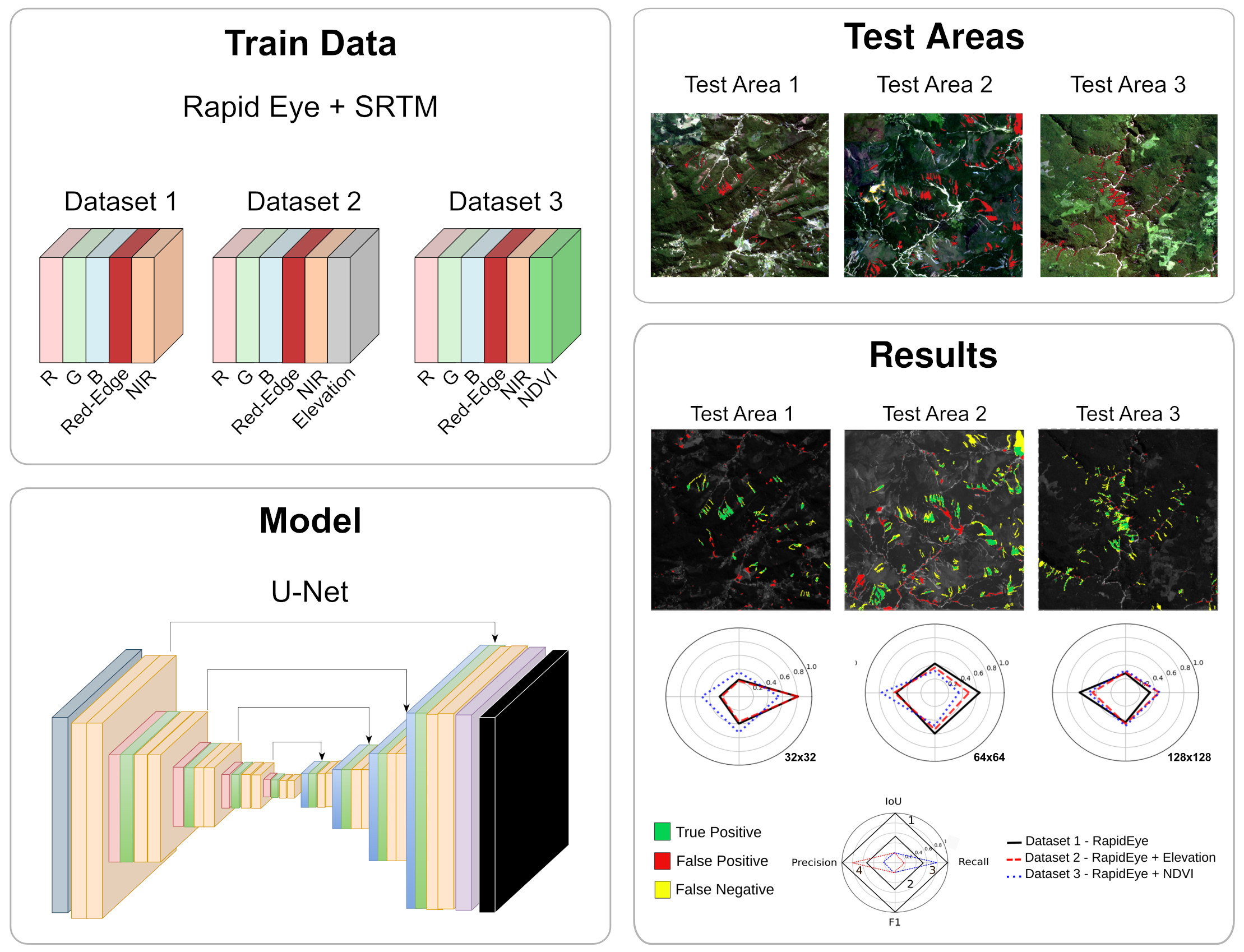
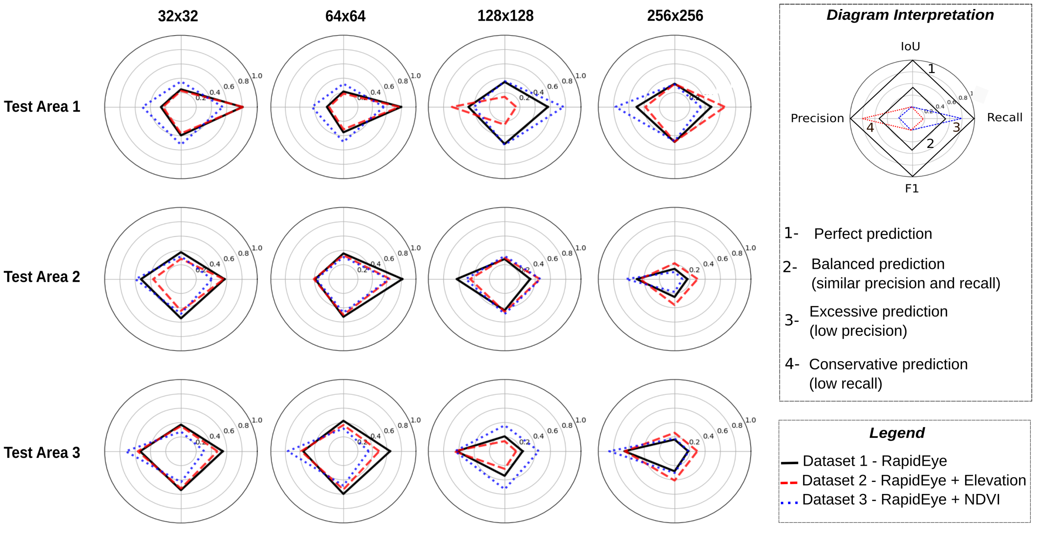
- Evaluation of model generalization in areas with different scene complexity in Brazil;
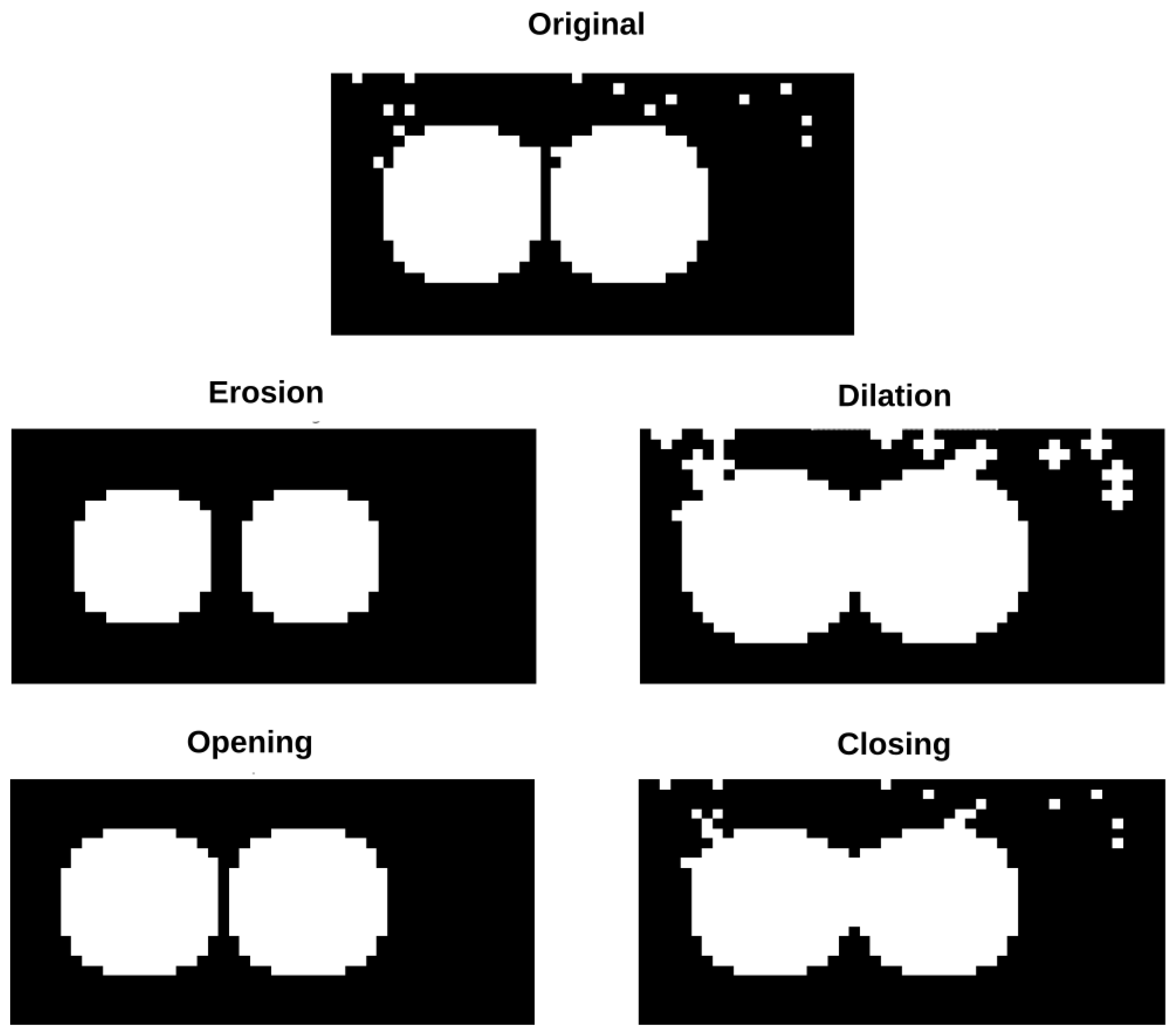
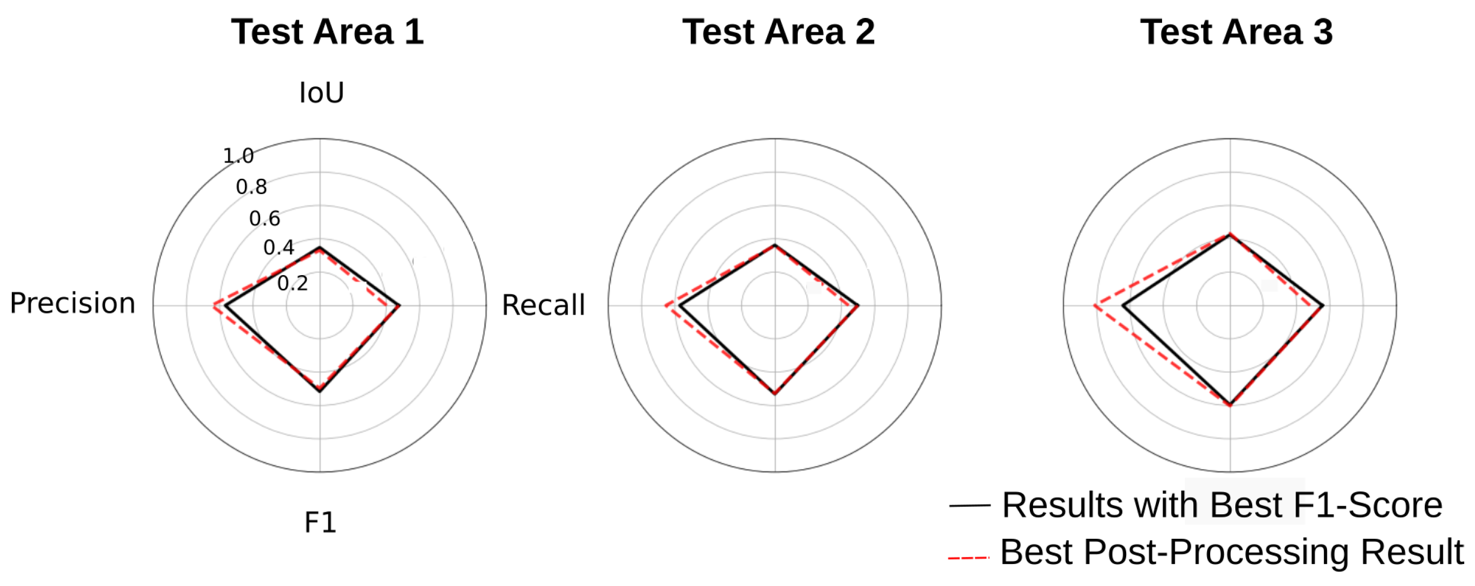
- Evaluation of binary opening, closing, dilation, and erosion as post-processing techniques;
- Evaluation of how different patch sizes affect model generalization;
- Evaluation of different datasets on model generalization.
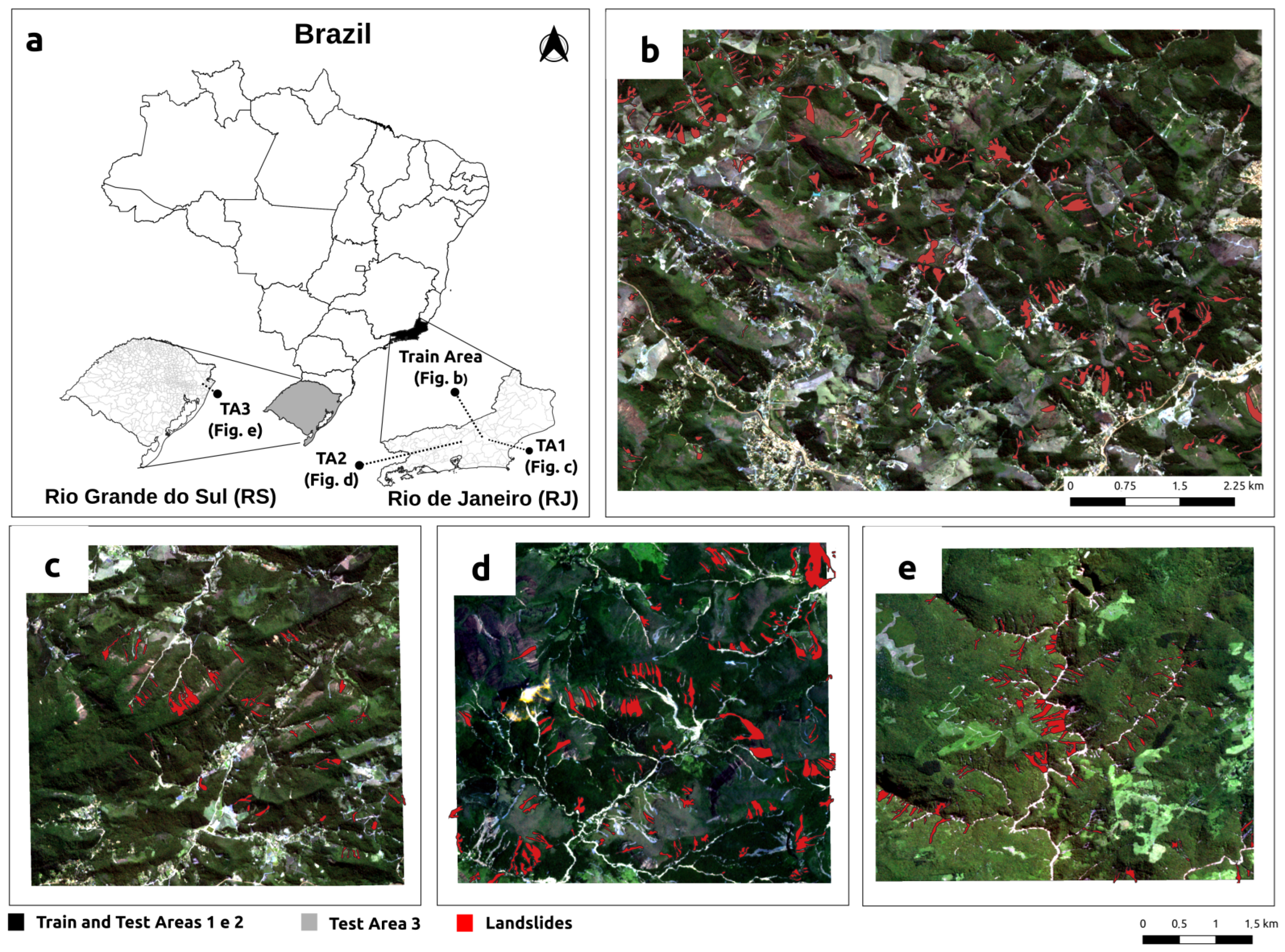
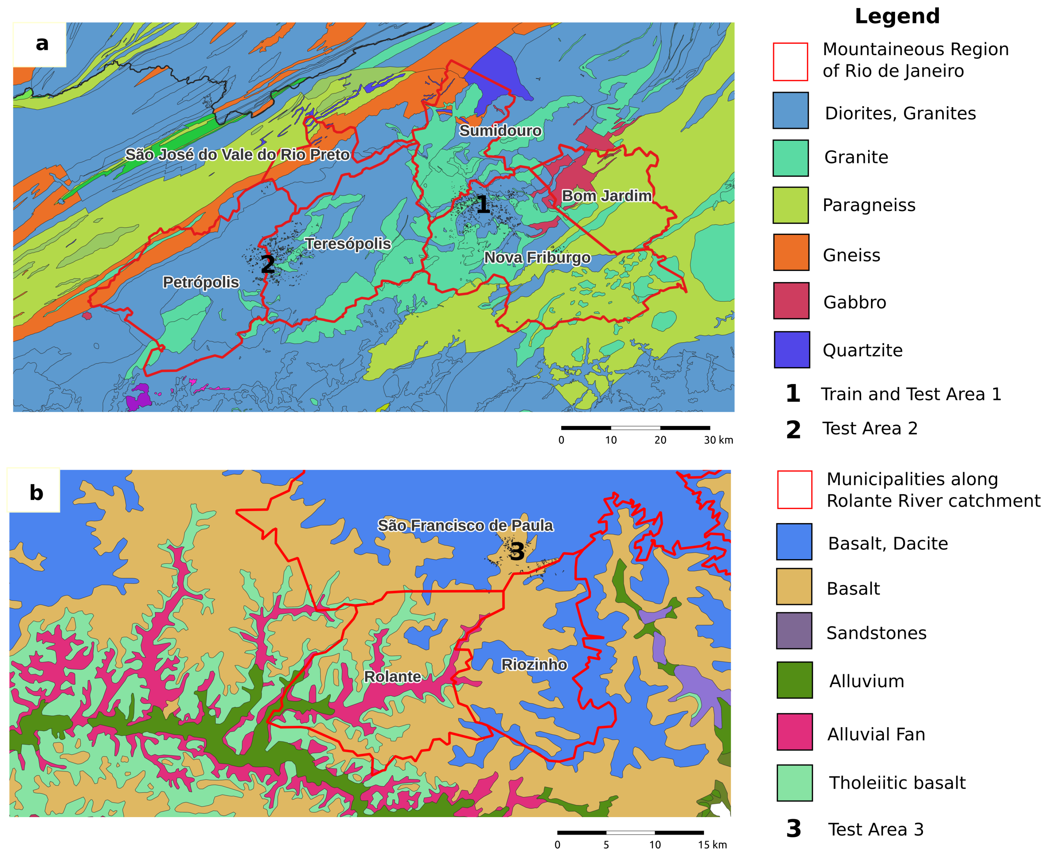
2. Study Areas
2.1. Nova Friburgo and Teresópolis
2.2. Rolante
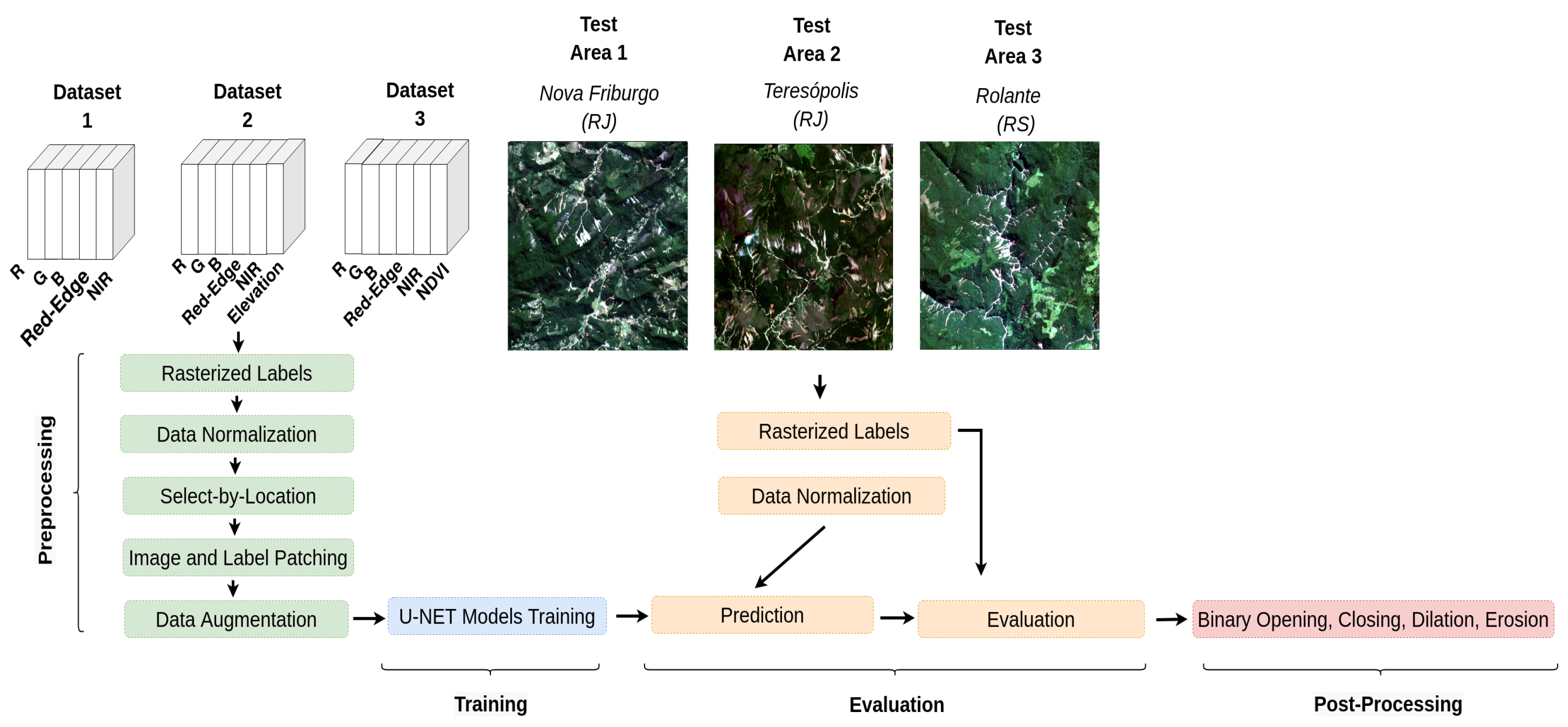
3. Methodology
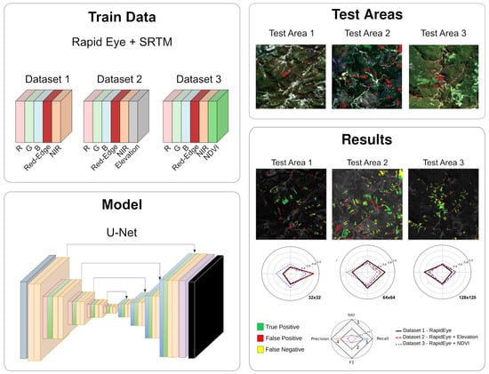
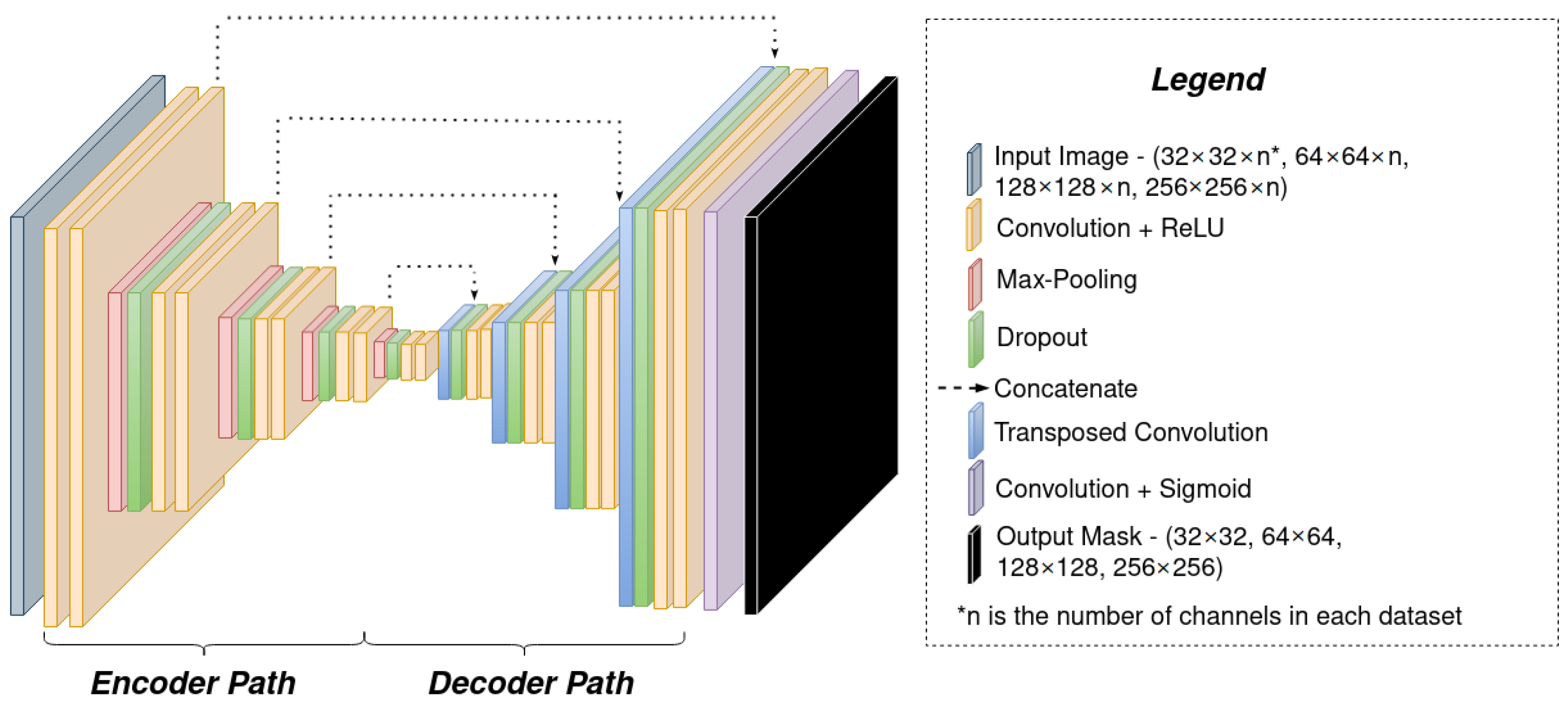
3.1. U-Net
3.2. Validation Metrics
3.3. Post-Processing
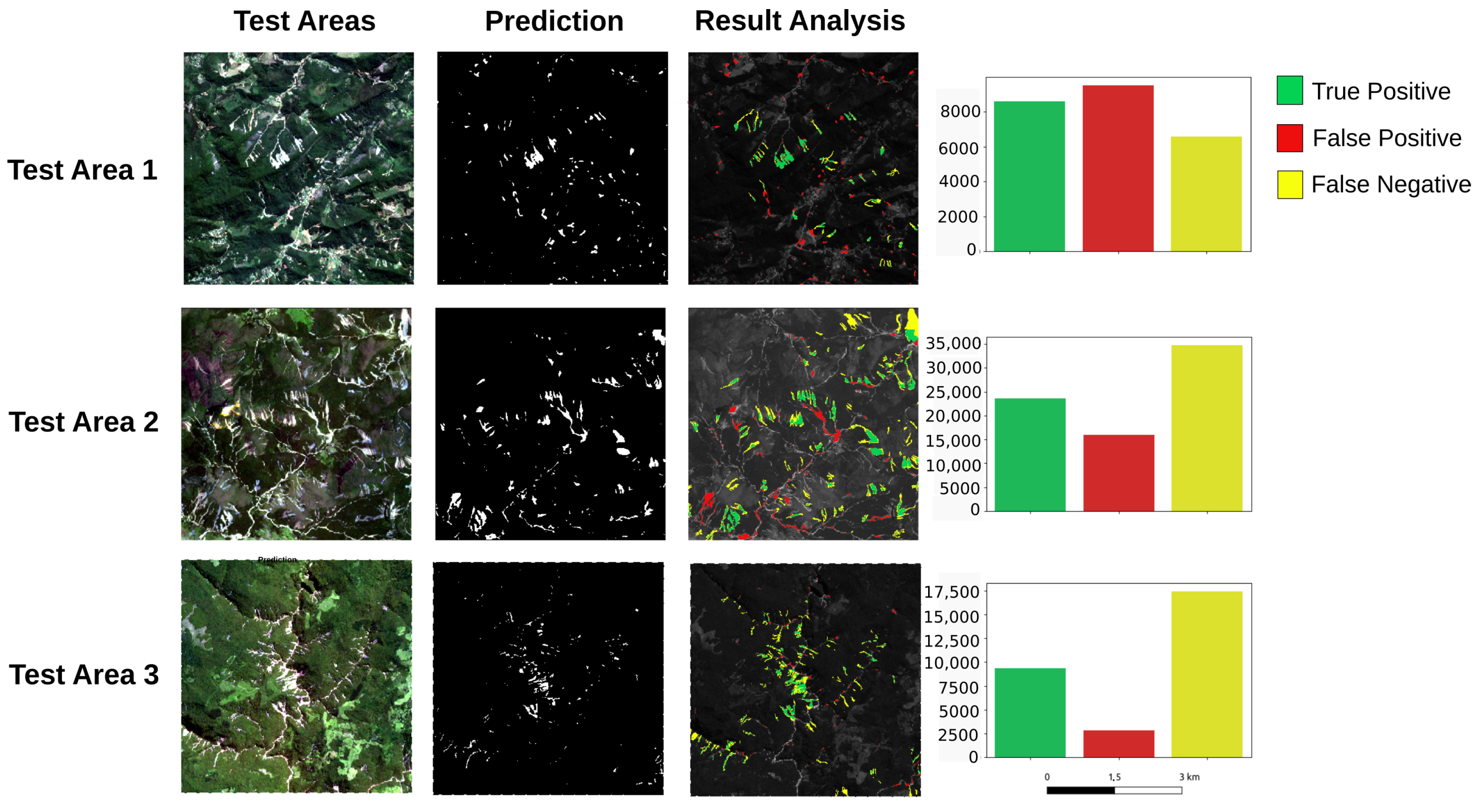
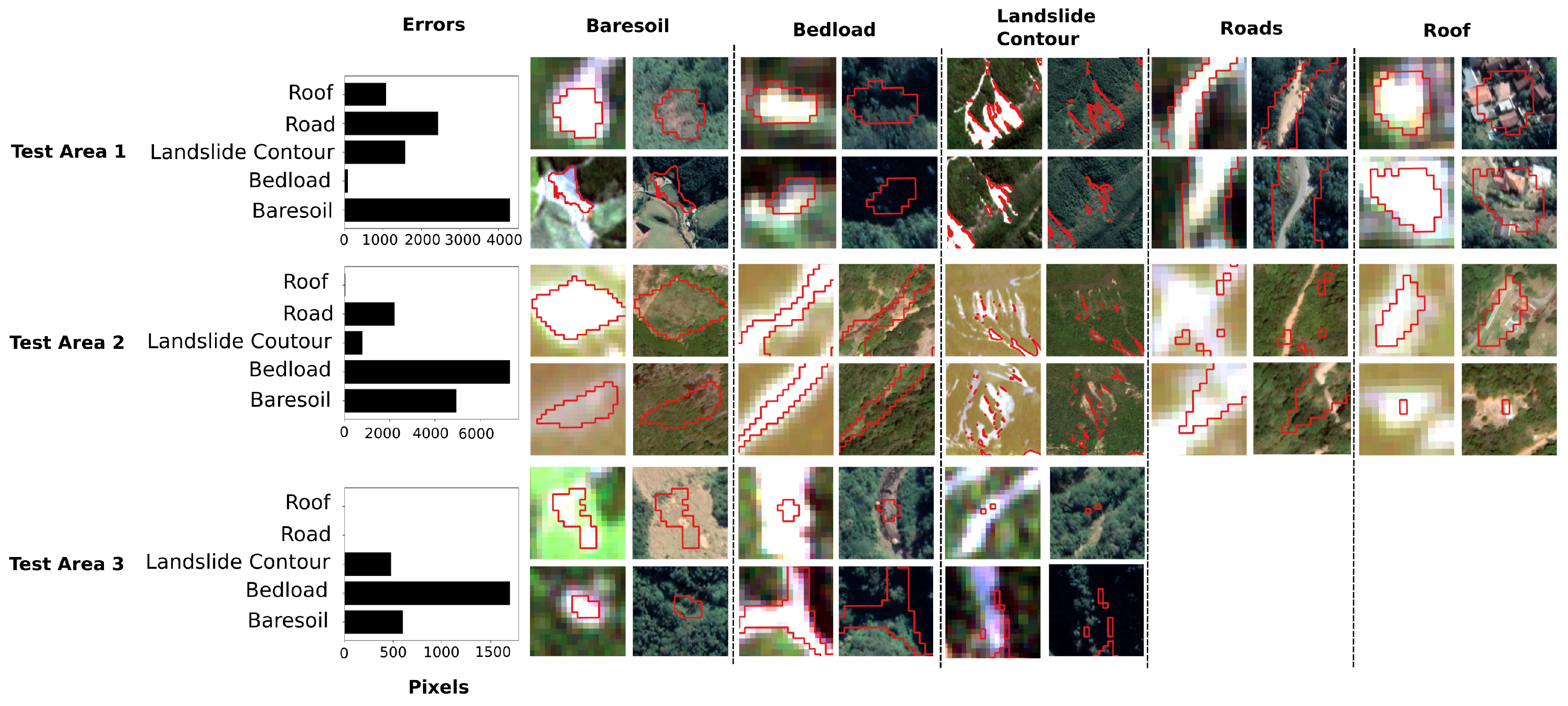
4. Results and Discussion
5. Conclusions
Supplementary Materials
Author Contributions
Funding
Data Availability Statement
Acknowledgments
Conflicts of Interest
References
- Metternicht, G.; Hurni, L.; Gogu, R. Remote sensing of landslides: An analysis of the potential contribution to geo-spatial systems for hazard assessment in mountainous environments. Remote Sens. Environ. 2005, 98, 284–303. [Google Scholar] [CrossRef]
- Froude, M.J.; Petley, D.N. Global fatal landslide occurrence from 2004 to 2016. Nat. Hazards Earth Syst. Sci. 2018, 18, 2161–2181. [Google Scholar] [CrossRef] [Green Version]
- Schuster, R.L.; Highland, L.M. The Third Hans Cloos Lecture. Urban landslides: Socioeconomic impacts and overview of mitigative strategies. Bull. Eng. Geol. Environ. 2007, 66, 1–27. [Google Scholar] [CrossRef]
- Yi, Y.; Zhang, Z.; Zhang, W.; Zhang, C.; Li, W.; Zhao, T. Semantic segmentation of urban buildings from VHR remote sensing imagery using a deep convolutional neural network. Remote Sens. 2019, 11, 1774. [Google Scholar] [CrossRef] [Green Version]
- Hong, H.; Chen, W.; Xu, C.; Youssef, A.M.; Pradhan, B.; Tien Bui, D. Rainfall-induced landslide susceptibility assessment at the Chongren area (China) using frequency ratio, certainty factor, and index of entropy. Geocarto Int. 2017, 32, 139–154. [Google Scholar] [CrossRef]
- Alexander, D.E. A brief survey of GIS in mass-movement studies, with reflections on theory and methods. Geomorphology 2008, 94, 261–267. [Google Scholar] [CrossRef]
- Zhong, C.; Liu, Y.; Gao, P.; Chen, W.; Li, H.; Hou, Y.; Nuremanguli, T.; Ma, H. Landslide mapping with remote sensing: Challenges and opportunities. Int. J. Remote Sens. 2019, 41, 1555–1581. [Google Scholar] [CrossRef]
- Tominaga, L.K.; Santoro, J.; Amaral, R. Desastres Naturais; Instituto Geológico: São Paulo, Brazil, 2009. [Google Scholar]
- CRED. EM-DAT: The International Emergency Disasters Database. 2022. Available online: https://www.emdat.be/ (accessed on 1 May 2022).
- Coelho-Netto, A.L.; de Souza Avelar, A.; Lacerda, W.A. Landslides and disasters in southeastern and southern Brazil. Dev. Earth Surf. Process. 2009, 13, 223–243. [Google Scholar]
- Netto, A.L.C.; Sato, A.M.; de Souza Avelar, A.; Vianna, L.G.G.; Araújo, I.S.; Ferreira, D.L.; Lima, P.H.; Silva, A.P.A.; Silva, R.P. January 2011: The extreme landslide disaster in Brazil. In Landslide Science and Practice; Springer: Berlin/Heidelberg, Germany, 2013; pp. 377–384. [Google Scholar]
- Vieira, B.C.; Gramani, M.F. Serra do Mar: The most “tormented” relief in Brazil. In Landscapes and Landforms of Brazil; Springer: Berlin/Heidelberg, Germany, 2015; pp. 285–297. [Google Scholar]
- Mondini, A.C.; Santangelo, M.; Rocchetti, M.; Rossetto, E.; Manconi, A.; Monserrat, O. Sentinel-1 SAR Amplitude Imagery for Rapid Landslide Detection. Remote Sens. 2019, 11, 760. [Google Scholar] [CrossRef] [Green Version]
- Guzzetti, F.; Mondini, A.C.; Cardinali, M.; Fiorucci, F.; Santangelo, M.; Chang, K.T. Landslide inventory maps: New tools for an old problem. Earth-Sci. Rev. 2012, 112, 42–66. [Google Scholar] [CrossRef] [Green Version]
- Catani, F.; Tofani, V.; Lagomarsino, D. Spatial patterns of landslide dimension: A tool for magnitude mapping. Geomorphology 2016, 273, 361–373. [Google Scholar] [CrossRef] [Green Version]
- Mavroulis, S.; Diakakis, M.; Kranis, H.; Vassilakis, E.; Kapetanidis, V.; Spingos, I.; Kaviris, G.; Skourtsos, E.; Voulgaris, N.; Lekkas, E. Inventory of Historical and Recent Earthquake-Triggered Landslides and Assessment of Related Susceptibility by GIS-Based Analytic Hierarchy Process: The Case of Cephalonia (Ionian Islands, Western Greece). Appl. Sci. 2022, 12, 2895. [Google Scholar] [CrossRef]
- Shao, X.; Ma, S.; Xu, C.; Shen, L.; Lu, Y. Inventory, distribution and geometric characteristics of landslides in Baoshan City, Yunnan Province, China. Sustainability 2020, 12, 2433. [Google Scholar] [CrossRef] [Green Version]
- Ardizzone, F.; Basile, G.; Cardinali, M.; Casagli, N.; Del Conte, S.; Del Ventisette, C.; Fiorucci, F.; Garfagnoli, F.; Gigli, G.; Guzzetti, F.; et al. Landslide inventory map for the Briga and the Giampilieri catchments, NE Sicily, Italy. J. Maps 2012, 8, 176–180. [Google Scholar] [CrossRef] [Green Version]
- Conforti, M.; Muto, F.; Rago, V.; Critelli, S. Landslide inventory map of north-eastern Calabria (South Italy). J. Maps 2014, 10, 90–102. [Google Scholar] [CrossRef]
- Dias, H.C.; Hölbling, D.W.; Grohmann, C.H. Landslide inventory mapping in Brazil: Status and challenges. In Proceedings of the XIII International Symposium on Landslides, virtual, 22–26 February 2021. [Google Scholar]
- Marcelino, E.V.; Formagio, A.R. Análise comparativa entre métodos heurísticos de mapeamento de áreas susceptíveis a escorregamento. Simpósio Bras. Desastr. Nat. 2004, 1, 392–407. [Google Scholar]
- Schulz, W.H. Landslide susceptibility revealed by LIDAR imagery and historical records, Seattle, Washington. Eng. Geol. 2007, 89, 67–87. [Google Scholar] [CrossRef]
- Kawabata, D.; Bandibas, J. Landslide susceptibility mapping using geological data, a DEM from ASTER images and an Artificial Neural Network (ANN). Geomorphology 2009, 113, 97–109. [Google Scholar] [CrossRef]
- Chen, H.; Zeng, Z. Deformation prediction of landslide based on improved back-propagation neural network. Cogn. Comput. 2013, 5, 56–62. [Google Scholar] [CrossRef]
- Du, J.C.; Teng, H.C. 3D laser scanning and GPS technology for landslide earthwork volume estimation. Autom. Constr. 2007, 16, 657–663. [Google Scholar] [CrossRef]
- Lingua, A.; Piatti, D.; Rinaudo, F. Remote monitoring of a landslide using an integration of GB-INSAR and LIDAR techniques. Int. Arch. Photogramm. Remote Sens. Spat. Inf. Sci. 2008, 37, 133–139. [Google Scholar]
- Baldo, M.; Bicocchi, C.; Chiocchini, U.; Giordan, D.; Lollino, G. LIDAR monitoring of mass wasting processes: The Radicofani landslide, Province of Siena, Central Italy. Geomorphology 2009, 105, 193–201. [Google Scholar] [CrossRef]
- Jaboyedoff, M.; Oppikofer, T.; Abellán, A.; Derron, M.H.; Loye, A.; Metzger, R.; Pedrazzini, A. Use of LIDAR in landslide investigations: A review. Nat. Hazards 2012, 61, 5–28. [Google Scholar] [CrossRef] [Green Version]
- Brideau, M.A.; McDougall, S.; Stead, D.; Evans, S.G.; Couture, R.; Turner, K. Three-dimensional distinct element modelling and dynamic runout analysis of a landslide in gneissic rock, British Columbia, Canada. Bull. Eng. Geol. Environ. 2012, 71, 467–486. [Google Scholar] [CrossRef]
- Ghuffar, S.; Székely, B.; Roncat, A.; Pfeifer, N. Landslide displacement monitoring using 3D range flow on airborne and terrestrial LiDAR data. Remote Sens. 2013, 5, 2720–2745. [Google Scholar] [CrossRef] [Green Version]
- Casagli, N.; Cigna, F.; Bianchini, S.; Hölbling, D.; Füreder, P.; Righini, G.; Del Conte, S.; Friedl, B.; Schneiderbauer, S.; Iasio, C.; et al. Landslide mapping and monitoring by using radar and optical remote sensing: Examples from the EC-FP7 project SAFER. Remote Sens. Appl. Soc. Environ. 2016, 4, 92–108. [Google Scholar] [CrossRef] [Green Version]
- Hsiao, K.; Liu, J.; Yu, M.; Tseng, Y. Change detection of landslide terrains using ground-based LiDAR data. In Proceedings of the XXth ISPRS Congress, Istanbul, Turkey, Commission VII, WG, Istanbul, Turkey, 12–13 July 2004; Volume 7, p. 5. [Google Scholar]
- McKean, J.; Roering, J. Objective landslide detection and surface morphology mapping using high-resolution airborne laser altimetry. Geomorphology 2004, 57, 331–351. [Google Scholar] [CrossRef]
- Glenn, N.F.; Streutker, D.R.; Chadwick, D.J.; Thackray, G.D.; Dorsch, S.J. Analysis of LiDAR-derived topographic information for characterizing and differentiating landslide morphology and activity. Geomorphology 2006, 73, 131–148. [Google Scholar] [CrossRef]
- Dewitte, O.; Jasselette, J.C.; Cornet, Y.; Van Den Eeckhaut, M.; Collignon, A.; Poesen, J.; Demoulin, A. Tracking landslide displacements by multi-temporal DTMs: A combined aerial stereophotogrammetric and LIDAR approach in western Belgium. Eng. Geol. 2008, 99, 11–22. [Google Scholar] [CrossRef]
- Kasai, M.; Ikeda, M.; Asahina, T.; Fujisawa, K. LiDAR-derived DEM evaluation of deep-seated landslides in a steep and rocky region of Japan. Geomorphology 2009, 113, 57–69. [Google Scholar] [CrossRef]
- Liu, J.K.; Chang, K.T.; Rau, J.Y.; Hsu, W.C.; Liao, Z.Y.; Lau, C.C.; Shih, T.Y. The geomorphometry of rainfall-induced landslides in taiwan obtained by airborne lidar and digital photography. In Geoscience and Remote Sensing; In-Tech, Inc.: Garching Bei München, Germany, 2009. [Google Scholar]
- Burns, W.J.; Coe, J.A.; Kaya, B.S.; Ma, L. Analysis of elevation changes detected from multi-temporal LiDAR surveys in forested landslide terrain in western Oregon. Environ. Eng. Geosci. 2010, 16, 315–341. [Google Scholar] [CrossRef]
- Ventura, G.; Vilardo, G.; Terranova, C.; Sessa, E.B. Tracking and evolution of complex active landslides by multi-temporal airborne LiDAR data: The Montaguto landslide (Southern Italy). Remote Sens. Environ. 2011, 115, 3237–3248. [Google Scholar] [CrossRef]
- Van Westen, C.J.; Castellanos, E.; Kuriakose, S.L. Spatial data for landslide susceptibility, hazard, and vulnerability assessment: An overview. Eng. Geol. 2008, 102, 112–131. [Google Scholar] [CrossRef]
- Korup, O.; Stolle, A. Landslide prediction from machine learning. Geol. Today 2014, 30, 26–33. [Google Scholar] [CrossRef]
- Steger, S.; Brenning, A.; Bell, R.; Glade, T. The influence of systematically incomplete shallow landslide inventories on statistical susceptibility models and suggestions for improvements. Landslides 2017, 14, 1767–1781. [Google Scholar] [CrossRef] [Green Version]
- Nilsen, T.H. Preliminary Photointerpretation Map of Landslide and Other Surficial Deposits of the Concord 15-Minute Quadrangle and the Oakland West, Richmond, and Part of the San Quentin 7 1/2-Minute Quadrangles, Contra Costa and Alameda Counties, California; Technical Report; US Geological Survey: Reston, VA, USA, 1973.
- Guzzetti, F.; Carrara, A.; Cardinali, M.; Reichenbach, P. Landslide hazard evaluation: A review of current techniques and their application in a multi-scale study, Central Italy. Geomorphology 1999, 31, 181–216. [Google Scholar] [CrossRef]
- Van Den Eeckhaut, M.; Poesen, J.; Verstraeten, G.; Vanacker, V.; Moeyersons, J.; Nyssen, J.; Van Beek, L. The effectiveness of hillshade maps and expert knowledge in mapping old deep-seated landslides. Geomorphology 2005, 67, 351–363. [Google Scholar] [CrossRef]
- Booth, A.M.; Roering, J.J.; Perron, J.T. Automated landslide mapping using spectral analysis and high-resolution topographic data: Puget Sound lowlands, Washington, and Portland Hills, Oregon. Geomorphology 2009, 109, 132–147. [Google Scholar] [CrossRef]
- Burns, W.J.; Madin, I. Protocol for Inventory Mapping of Landslide Deposits from Light Detection and Ranging (LiDAR) Imagery. 2009. Available online: https://www.oregongeology.org/pubs/dds/slido/sp-42_onscreen.pdf (accessed on 1 May 2022).
- Roering, J.J.; Mackey, B.H.; Marshall, J.A.; Sweeney, K.E.; Deligne, N.I.; Booth, A.M.; Handwerger, A.L.; Cerovski-Darriau, C. ‘You are HERE’: Connecting the dots with airborne lidar for geomorphic fieldwork. Geomorphology 2013, 200, 172–183. [Google Scholar] [CrossRef]
- Scaioni, M.; Longoni, L.; Melillo, V.; Papini, M. Remote sensing for landslide investigations: An overview of recent achievements and perspectives. Remote Sens. 2014, 6, 9600–9652. [Google Scholar] [CrossRef] [Green Version]
- Van Den Eeckhaut, M.; Hervás, J.; Jaedicke, C.; Malet, J.P.; Montanarella, L.; Nadim, F. Statistical modelling of Europe-wide landslide susceptibility using limited landslide inventory data. Landslides 2012, 9, 357–369. [Google Scholar] [CrossRef]
- Knevels, R.; Petschko, H.; Leopold, P.; Brenning, A. Geographic object-based image analysis for automated landslide detection using open source GIS software. ISPRS Int. J. Geo-Inf. 2019, 8, 551. [Google Scholar] [CrossRef] [Green Version]
- Li, Y.; Chen, W. Landslide susceptibility evaluation using hybrid integration of evidential belief function and machine learning techniques. Water 2020, 12, 113. [Google Scholar] [CrossRef] [Green Version]
- Wang, Y.; Fang, Z.; Wang, M.; Peng, L.; Hong, H. Comparative study of landslide susceptibility mapping with different recurrent neural networks. Comput. Geosci. 2020, 138, 104445. [Google Scholar] [CrossRef]
- Xu, C. Preparation of earthquake-triggered landslide inventory maps using remote sensing and GIS technologies: Principles and case studies. Geosci. Front. 2015, 6, 825–836. [Google Scholar] [CrossRef] [Green Version]
- Yu, B.; Chen, F.; Xu, C. Landslide detection based on contour-based deep learning framework in case of national scale of Nepal in 2015. Comput. Geosci. 2020, 135, 104388. [Google Scholar] [CrossRef]
- Blaschke, T. Object based image analysis for remote sensing. ISPRS J. Photogramm. Remote Sens. 2010, 65, 2–16. [Google Scholar] [CrossRef] [Green Version]
- Hossain, M.D.; Chen, D. Segmentation for Object-Based Image Analysis (OBIA): A review of algorithms and challenges from remote sensing perspective. ISPRS J. Photogramm. Remote Sens. 2019, 150, 115–134. [Google Scholar] [CrossRef]
- Stumpf, A.; Kerle, N. Object-oriented mapping of landslides using Random Forests. Remote Sens. Environ. 2011, 115, 2564–2577. [Google Scholar] [CrossRef]
- Blaschke, T.; Hay, G.J.; Kelly, M.; Lang, S.; Hofmann, P.; Addink, E.; Feitosa, R.Q.; Van der Meer, F.; Van der Werff, H.; Van Coillie, F.; et al. Geographic object-based image analysis–towards a new paradigm. ISPRS J. Photogramm. Remote Sens. 2014, 87, 180–191. [Google Scholar] [CrossRef] [Green Version]
- Prakash, N.; Manconi, A.; Loew, S. Mapping landslides on EO data: Performance of deep learning models vs. traditional machine learning models. Remote Sens. 2020, 12, 346. [Google Scholar] [CrossRef] [Green Version]
- Ghorbanzadeh, O.; Blaschke, T.; Gholamnia, K.; Meena, S.R.; Tiede, D.; Aryal, J. Evaluation of different machine learning methods and deep-learning convolutional neural networks for landslide detection. Remote Sens. 2019, 11, 196. [Google Scholar] [CrossRef] [Green Version]
- Peng, D.; Zhang, Y.; Guan, H. End-to-End Change Detection for High Resolution Satellite Images Using Improved UNet++. Remote Sens. 2019, 11, 1382. [Google Scholar] [CrossRef] [Green Version]
- Zhu, X.X.; Tuia, D.; Mou, L.; Xia, G.S.; Zhang, L.; Xu, F.; Fraundorfer, F. Deep learning in remote sensing: A comprehensive review and list of resources. IEEE Geosci. Remote Sens. Mag. 2017, 5, 8–36. [Google Scholar] [CrossRef] [Green Version]
- Long, J.; Shelhamer, E.; Darrell, T. Fully convolutional networks for semantic segmentation. In Proceedings of the IEEE Conference on Computer Vision and Pattern Recognition, Boston, MA, USA, 7–12 June 2015; pp. 3431–3440. [Google Scholar]
- Radovic, M.; Adarkwa, O.; Wang, Q. Object recognition in aerial images using convolutional neural networks. J. Imaging 2017, 3, 21. [Google Scholar] [CrossRef]
- Sameen, M.I.; Pradhan, B. Landslide Detection Using Residual Networks and the Fusion of Spectral and Topographic Information. IEEE Access 2019, 7, 114363–114373. [Google Scholar] [CrossRef]
- Yi, Y.; Zhang, W. A new deep-learning-based approach for earthquake-triggered landslide detection from single-temporal RapidEye satellite imagery. IEEE J. Sel. Top. Appl. Earth Obs. Remote Sens. 2020, 13, 6166–6176. [Google Scholar] [CrossRef]
- Prakash, N.; Manconi, A.; Loew, S. A new strategy to map landslides with a generalized convolutional neural network. Sci. Rep. 2021, 11, 1–15. [Google Scholar] [CrossRef]
- Pradhan, B.; Seeni, M.I.; Nampak, H. Integration of LiDAR and QuickBird data for automatic landslide detection using object-based analysis and random forests. In Laser Scanning Applications in Landslide Assessment; Springer: Berlin/Heidelberg, Germany, 2017; pp. 69–81. [Google Scholar]
- Avelar, A.S.; Netto, A.L.C.; Lacerda, W.A.; Becker, L.B.; Mendonça, M.B. Mechanisms of the recent catastrophic landslides in the mountainous range of Rio de Janeiro, Brazil. In Landslide Science and Practice; Springer: Berlin/Heidelberg, Germany, 2013; pp. 265–270. [Google Scholar]
- Dantas, M.E. Geomorfologia do Estado do Rio de Janeiro; CPRM. Estudo Geoambiental do Estado do Rio de Janeiro: Brasília, Brazil, 2001. [Google Scholar]
- Tupinambá, M.; Heilbron, M.; Duarte, B.P.; de Almeida, J.C.H.; Valladares, C.S.; Pacheco, B.T.; dos Santos Salomão, M.; Conceição, F.R.; da Silva, L.G.E.; de Almeida, C.G.; et al. Mapa Geológico Folha Nova Friburgo SF-23-Z-B-II; Technical Report; CPRM—Serviço Geológico do Brasil: Rio de Janeirom, Brazil, 2012. [Google Scholar]
- Köppen, W. Das Geographische System der Klimate; Gerbrüder Bornträger: Stuttgart, Germany, 1936; Volume 1, Das geographische System der Klimate; pp. 1–44. [Google Scholar]
- Sobral, B.S.; Oliveira-Júnior, J.F.; Gois, G.; de Bodas Terassi, P.M.; Muniz-Júnior, J.G.R. Variabilidade espaço-temporal e interanual da chuva no estado do Rio de Janeiro. Rev. Bras. Climatol. 2018, 22. [Google Scholar] [CrossRef] [Green Version]
- Uehara, T.D.T.; Correa, S.P.L.P.; Quevedo, R.P.; Körting, T.S.; Dutra, L.V.; Rennó, C.D. Classification algorithms comparison for landslide scars. GEOINFO 2019, 20, 158. [Google Scholar]
- Gameiro, S.; Quevedo, R.P.; Oliveira, G.; Ruiz, L.; Guasselli, L. Análise e correlação de atributos morfométricos e sua influência nos movimentos de massa ocorridos na Bacia do Rio Rolante, RS. In Proceedings of the Anais do XIX Simpósio Brasileiro de Sensoriamento Remoto, Santos, Brazil, 14–17 April 2019; pp. 2880–2883. [Google Scholar]
- Quevedo, R.P.; Oliveira, G.; Gameiro, S.; Ruiz, L.; Guasselli, L. Modelagem de áreas suscetíveis a movimentos de massa com redes neurais artificiais. In Proceedings of the Anais do XIX Simpósio Brasileiro de Sensoriamento Remoto, Santos, Brazil, 14–17 April 2019; Volume 19, pp. 2910–2913. [Google Scholar]
- Quevedo, R.P.; Guasselli, L.A.; Oliveira, G.G.; Ruiz, L.F.C. Modelagem de áreas suscetíveis a movimentos de massa: Avaliação comparativa de técnicas de amostragem, aprendizado de máquina e modelos digitais de elevação. Geociências 2020, 38, 781–795. [Google Scholar] [CrossRef]
- Farr, T.G.; Rosen, P.A.; Caro, E.; Crippen, R.; Duren, R.; Hensley, S.; Kobrick, M.; Paller, M.; Rodriguez, E.; Roth, L.; et al. The Shuttle Radar Topography Mission. Rev. Geophys. 2007, 45, RG2004. [Google Scholar] [CrossRef] [Green Version]
- RapidEye, A. Satellite imagery product specifications. In Satellite Imagery Product Specifications: Version; BlackBridge: Lethbridge, AB, Canada, 2011. [Google Scholar]
- Planet Team. Planet Application Program Interface: In Space for Life on Earth. 2017. Available online: https://api.planet.com (accessed on 1 May 2020).
- Tucker, C.J. Red and photographic infrared linear combinations for monitoring vegetation. Remote Sens. Environ. 1979, 8, 127–150. [Google Scholar] [CrossRef] [Green Version]
- Rasterio: Geospatial Raster I/O for Python Programmers. 2013. Available online: https://github.com/rasterio/rasterio (accessed on 1 May 2022).
- Dixit, M.; Kwitt, R.; Niethammer, M.; Vasconcelos, N. Aga: Attribute-guided augmentation. In Proceedings of the IEEE Conference on Computer Vision and Pattern Recognition, Honolulu, HI, USA, 21–26 July 2017; pp. 7455–7463. [Google Scholar]
- Ronneberger, O.; Fischer, P.; Brox, T. U-net: Convolutional networks for biomedical image segmentation. In Proceedings of the International Conference on Medical Image Computing and Computer-Assisted Intervention, Munich, Germany, 5–9 October 2015; pp. 234–241. [Google Scholar]
- Quinn, J.; McEachen, J.; Fullan, M.; Gardner, M.; Drummy, M. Dive into Deep Learning: Tools for Engagement; Corwin Press: Thousand Oaks, CA, USA, 2019. [Google Scholar]
- Srivastava, N.; Hinton, G.; Krizhevsky, A.; Sutskever, I.; Salakhutdinov, R. Dropout: A simple way to prevent neural networks from overfitting. J. Mach. Learn. Res. 2014, 15, 1929–1958. [Google Scholar]
- Keras. 2015. Available online: https://keras.io/ (accessed on 1 May 2022).
- Abadi, M.; Agarwal, A.; Barham, P.; Brevdo, E.; Chen, Z.; Citro, C.; Corrado, G.S.; Davis, A.; Dean, J.; Devin, M.; et al. TensorFlow: Large-Scale Machine Learning on Heterogeneous Systems. 2015. Available online: tensorflow.org (accessed on 1 May 2022).
- Ghorbanzadeh, O.; Tiede, D.; Dabiri, Z.; Sudmanns, M.; Lang, S. Dwelling extraction in refugee camps using cnn–first experiences and lessons learnt. Int. Arch. Photogramm. Remote Sens. Spat. Inf. Sci. 2018. [Google Scholar] [CrossRef] [Green Version]
- Guirado, E.; Tabik, S.; Alcaraz-Segura, D.; Cabello, J.; Herrera, F. Deep-learning convolutional neural networks for scattered shrub detection with google earth imagery. arXiv 2017, arXiv:1706.00917. [Google Scholar]
- Van der Walt, S.; Schönberger, J.L.; Nunez-Iglesias, J.; Boulogne, F.; Warner, J.D.; Yager, N.; Gouillart, E.; Yu, T. Scikit-image: Image processing in Python. PeerJ 2014, 2, e453. [Google Scholar] [CrossRef]
- Soares, L.P.; Dias, H.C.; Grohmann, C.H. Landslide segmentation with u-net: Evaluating different sampling methods and patch sizes. arXiv 2020, arXiv:2007.06672. [Google Scholar]
- Hughes, G. On the mean accuracy of statistical pattern recognizers. IEEE Trans. Inf. Theory 1968, 14, 55–63. [Google Scholar] [CrossRef] [Green Version]
- Verstraete, M.M.; Pinty, B. Designing optimal spectral indexes for remote sensing applications. IEEE Trans. Geosci. Remote Sens. 1996, 34, 1254–1265. [Google Scholar] [CrossRef]
- Mondini, A.; Guzzetti, F.; Reichenbach, P.; Rossi, M.; Cardinali, M.; Ardizzone, F. Semi-automatic recognition and mapping of rainfall induced shallow landslides using optical satellite images. Remote Sens. Environ. 2011, 115, 1743–1757. [Google Scholar] [CrossRef]
- Lu, P.; Qin, Y.; Li, Z.; Mondini, A.C.; Casagli, N. Landslide mapping from multi-sensor data through improved change detection-based Markov random field. Remote Sens. Environ. 2019, 231, 111235. [Google Scholar] [CrossRef]
- Qi, W.; Wei, M.; Yang, W.; Xu, C.; Ma, C. Automatic mapping of landslides by the ResU-net. Remote Sens. 2020, 12, 2487. [Google Scholar] [CrossRef]
- Altman, N.; Krzywinski, M. The curse (s) of dimensionality. Nat. Methods 2018, 15, 399–400. [Google Scholar] [CrossRef] [PubMed]
- Ghorbanzadeh, O.; Meena, S.R.; Abadi, H.S.S.; Piralilou, S.T.; Zhiyong, L.; Blaschke, T. Landslide Mapping Using Two Main Deep-Learning Convolution Neural Network Streams Combined by the Dempster–Shafer Model. IEEE J. Sel. Top. Appl. Earth Obs. Remote Sens. 2020, 14, 452–463. [Google Scholar] [CrossRef]
- Krizhevsky, A.; Sutskever, I.; Hinton, G.E. Imagenet classification with deep convolutional neural networks. Adv. Neural Inf. Process. Syst. 2012, 25, 1097–1105. [Google Scholar] [CrossRef]
- Bottou, L.; Cortes, C.; Denker, J.S.; Drucker, H.; Guyon, I.; Jackel, L.D.; LeCun, Y.; Muller, U.A.; Sackinger, E.; Simard, P.; et al. Comparison of classifier methods: A case study in handwritten digit recognition. In Proceedings of the 12th IAPR International Conference on Pattern Recognition, Vol. 3-Conference C: Signal Processing (Cat. No. 94CH3440-5), Jerusalem, Israel, 9–13 October 1994; Volume 2, pp. 77–82. [Google Scholar]
- Helber, P.; Bischke, B.; Dengel, A.; Borth, D. Eurosat: A novel dataset and deep learning benchmark for land use and land cover classification. IEEE J. Sel. Top. Appl. Earth Obs. Remote Sens. 2019, 12, 2217–2226. [Google Scholar] [CrossRef] [Green Version]
- Yang, Y.; Newsam, S. Bag-of-visual-words and spatial extensions for land-use classification. In Proceedings of the 18th SIGSPATIAL International Conference on Advances in Geographic Information Systems, San Jose, CA, USA, 2–5 November 2010; pp. 270–279. [Google Scholar]
- Xia, G.S.; Hu, J.; Hu, F.; Shi, B.; Bai, X.; Zhong, Y.; Zhang, L.; Lu, X. AID: A benchmark data set for performance evaluation of aerial scene classification. IEEE Trans. Geosci. Remote Sens. 2017, 55, 3965–3981. [Google Scholar] [CrossRef] [Green Version]
- Penatti, O.A.; Nogueira, K.; Dos Santos, J.A. Do deep features generalize from everyday objects to remote sensing and aerial scenes domains? In Proceedings of the IEEE Conference on Computer Vision and Pattern Recognition Workshops, Boston, MA, USA, 7–12 June 2015; pp. 44–51. [Google Scholar]


| Images | Acquisition Date | Number of |
|---|---|---|
| (RapidEye/SRTM) | Landslides | |
| Train Area (Nova Friburgo) | 10 January 2011/23 September 2014 | 455 |
| TA1 (Nova Friburgo) | 10 January 2011/23 September 2014 | 42 |
| TA2 (Teresópolis) | 20 January 2011/23 September 2014 | 117 |
| TA3 (Rolante) | 13 March 2017/23 September 2014 | 110 |
| Area | Operation | Recall | Precision | F1-Score | mIoU |
|---|---|---|---|---|---|
| TA1 | - | 0.57 | 0.47 | 0.52 | 0.35 |
| TA1 | Opening Erosion + Dilation Dilation + Erosion + Opening | 0.48 | 0.56 | 0.52 | 0.35 |
| TA2 | - | 0.50 | 0.57 | 0.53 | 0.36 |
| TA2 | Dilation Closing + Dilation Erosion + Opening + Closing | 0.44 | 0.65 | 0.53 | 0.36 |
| TA3 | - | 0.56 | 0.64 | 0.60 | 0.42 |
| TA3 | Dilation Closing + Dilation Erosion + Opening + Closing | 0.48 | 0.81 | 0.60 | 0.43 |
Publisher’s Note: MDPI stays neutral with regard to jurisdictional claims in published maps and institutional affiliations. |
© 2022 by the authors. Licensee MDPI, Basel, Switzerland. This article is an open access article distributed under the terms and conditions of the Creative Commons Attribution (CC BY) license (https://creativecommons.org/licenses/by/4.0/).
Share and Cite
Soares, L.P.; Dias, H.C.; Garcia, G.P.B.; Grohmann, C.H. Landslide Segmentation with Deep Learning: Evaluating Model Generalization in Rainfall-Induced Landslides in Brazil. Remote Sens. 2022, 14, 2237. https://doi.org/10.3390/rs14092237
Soares LP, Dias HC, Garcia GPB, Grohmann CH. Landslide Segmentation with Deep Learning: Evaluating Model Generalization in Rainfall-Induced Landslides in Brazil. Remote Sensing. 2022; 14(9):2237. https://doi.org/10.3390/rs14092237
Chicago/Turabian StyleSoares, Lucas Pedrosa, Helen Cristina Dias, Guilherme Pereira Bento Garcia, and Carlos Henrique Grohmann. 2022. "Landslide Segmentation with Deep Learning: Evaluating Model Generalization in Rainfall-Induced Landslides in Brazil" Remote Sensing 14, no. 9: 2237. https://doi.org/10.3390/rs14092237
APA StyleSoares, L. P., Dias, H. C., Garcia, G. P. B., & Grohmann, C. H. (2022). Landslide Segmentation with Deep Learning: Evaluating Model Generalization in Rainfall-Induced Landslides in Brazil. Remote Sensing, 14(9), 2237. https://doi.org/10.3390/rs14092237