Article

Diurnal Variations of Water Ice in the Martian Atmosphere Observed by Mars Climate Sounder

1
Planetary Environmental and Astrobiological Research Laboratory, School of Atmospheric Sciences, Sun Yat-sen University, Zhuhai 519082, China
2
CAS Center for Excellence in Comparative Planetology, Hefei 230026, China
3
CAS Key Laboratory of Geospace Environment, School of Earth and Space Sciences, University of Science and Technology of China, Hefei 230026, China
4
Key Laboratory of Space Weather, National Satellite Meteorological Center (National Center for Space Weather), China Meteorological Administration, Beijing 100081, China
5
Innovation Center for FengYun Meteorological Satellite (FYSIC), Beijing 100081, China
*
Author to whom correspondence should be addressed.
Remote Sens. 2022, 14(9), 2235; https://doi.org/10.3390/rs14092235
Submission received: 25 March 2022 / Revised: 2 May 2022 / Accepted: 4 May 2022 / Published: 6 May 2022
(This article belongs to the Special Issue Mars Remote Sensing)

Abstract

:
Simulation studies have proposed a significant thermal effect of water ice clouds on the Martian atmosphere and climate. However, previous studies focused more on seasonal variations but less on short-term changes. In this work, we used the MCS multi-local time data to investigate the water ice diurnal variations on Mars. We quantified its diurnal variations with amplitude and phase by applying the tidal fitting method to the water ice abundance. In addition, we found a close correlation (antiphase relation) between the thermal tide and water ice diurnal variations during the aphelion seasons that was not sensitive to both the background water ice and dust opacity but increased with the tidal amplitude. In the perihelion seasons, the antiphase relation was sensitive to the water ice and dust opacity, both affected by the dust storm activity. Finally, the statistic results suggested an unexpected low threshold of diurnal tide amplitude (2 to 3 K) for generating a relevant water ice diurnal variation, accounting for the ubiquitous water ice diurnal variations in the Martian atmosphere. These new observational results can help further understand the phase transition process between ice and vapor in the Martian atmosphere and better constrain the Martian global climate model in the future.

1. Introduction

Although the Martian atmosphere is thin, its thermodynamic processes share similarities with those on Earth, such as the thermal structure, the seasonal variation, coupling processes related to atmospheric waves, interactions with the surface, etc. [1,2]. A comparative study between the atmospheres of Mars and Earth provides new perspectives to understand the history and future of the Earth. The systematic investigation and understanding of the Martian atmospheric dynamics also help engineers guarantee the safety of future Mars missions [3,4].
The Martian surface is mainly covered with dust as a desert planet but still has water in the atmosphere, surface ice, and underground [5]. Vapor and ice are the two forms of water on Mars due to the low pressure (~1 percent of Earth’s sea-level pressure) and temperature (below freezing most of the time). As one of the life elements (e.g., water, methane, ozone, etc.) that may exist in a planetary atmosphere, water is of great significance in exploring extraterrestrial life. The distribution, transport, source, and sink of water are the basis of understanding and tracking the water-related biological elements on Mars. On the other hand, water vapor and ice clouds absorb and scatter solar and ground radiations and emit infrared radiation, altering the thermal structure of the atmosphere. Recent studies suggested that clouds have significant thermodynamic effects on the Martian atmosphere and climate [6,7,8,9,10].
Multiple spacecraft have focused on the water distribution and cloud particle sizes in the Martian atmosphere [11,12,13]. For example, the global-scaled spatial distribution and seasonal evolution of water vapor and water ice clouds have been well-investigated based on observations from Mars Global Surveyor (MGS) [14,15], Mars Reconnaissance Orbiter (MRO) [16,17], Odyssey [14], and Mars Express (MEX) [18,19,20]. Generally, the column water vapor abundance increases at high latitudes during the summer to its annual maximum in both the Northern and Southern Hemispheres. However, it decreases after the maximum near the summer solstice, with only a moderate increase at low latitudes during the equinoxes [21]. As for water ice clouds, two typical types, i.e., the tropical and polar hood clouds, are characterized and distinguished by their latitude distributions. The tropical ice cloud’s abundance, latitude, and altitude range significantly increase during the aphelian seasons (northern summer and early fall) while diminishing during the perihelion seasons, also called the aphelion cloud belt [22,23]. The north and south polar hood clouds tend to form during the fall and winter seasons of the corresponding hemisphere [24,25].
However, the Martian atmosphere’s water ice cloud structure and evolution are still incompletely understood. Although several numerical simulations have considered the formation and diurnal evolution of water ice clouds [26,27], observational studies have focused more on their seasonal variations and global distribution and less on their short-term changes. Recent observations showed rapid vertical transport or temporal changes in water vapor and ice cloud distribution during major dust storms [28,29,30]. The short-term burst of water vapor into the middle and upper atmospheres facilitates its escape, which is essential for understanding the evolution of the Martian atmospheric habitability. Simulations connected these short-term phenomena to the diurnal thermal tide—an intense, global, and diurnally varied atmospheric wave activity occurring across the Martian atmosphere [31,32,33,34]. The Martian thermal tides are vastly stronger and more critical than those on Earth because of the significant diurnal temperature variations [35]. In turn, the thermal effect of water ice clouds can also shape the phase transition of the thermal tide during a major dust storm, forming a close and complicated interactive relation between them [36]. The diurnal variations of the water ice cloud outside a major dust storm were only partially investigated based on 3 a.m. and 3 p.m. water ice retrievals from the Mars Climate Sounder (MCS) instrument onboard MRO [22,24,37]. For example, the observed north polar hood clouds are thicker in the nighttime than in the daytime, probably due to tidal-driven diurnal temperature differences or the nighttime polar vortex. In contrast, the south polar hood clouds have two cloud layers that may be separated by a tidally modulated temperature inversion [24,25]. In addition, the lower-atmosphere water ice opacity correlates with the temperature field, with the water ice maxima in the local temperature minima, further validating the tidal effect. However, analyses based on data at two local times are insufficient to distinguish the detailed variations within a day or to determine the phase (i.e., the local time of the maximum or minimum) of the water ice or temperature diurnal variations [36,38]. This makes it impossible to quantitatively study the diurnal variations of water ice clouds and their relationship with the diurnal thermal tide.
In recent years, MCS adopted a multi-local time observational strategy that could measure the atmospheric temperature, airborne dust, and water ice simultaneously and provide opportunities to determine the amplitude and phase information of thermal tides and aerosols diurnal variations [31,36,39]. In this work, we use the MCS multi-local time data of the entire Mars Year (MY) 33 to conduct the first comprehensive study on the diurnal variations of water ice global distribution and seasonal evolution. The main goal is to quantify the relationship between the thermal tides and diurnal variations of water ice and its general applicability in the real Mars atmosphere. The MCS multi-local time dataset makes it possible to perform the valid wave extraction method used by previous studies [31,38]. The comprehensive study of the global water ice diurnal variations will help to further understand the phase transition process between ice and vapor in the Martian atmosphere. These new observational results can also better constrain the Martian global climate model (MGCM), which is significant for understanding the entire Martian atmospheric environment and climate evolution.
The layout of the paper is as follows. Section 2 introduces the MCS dataset and its observational strategy that facilitate this work. The data analysis and nonlinear least square fitting method used to estimate the amplitude and phase of the water ice diurnal variations are also described. Section 3 shows the main characteristics of the water ice diurnal variations and their relations with the diurnal tide. Finally, Section 4 discusses the possible implications of the observed phenomenon, and Section 5 draws the main conclusions.

2. Data and Methods

2.1. MCS Dataset

This work uses the version 5 MCS dataset from the Planetary Data System. MCS has measured the thermal emissions of the Martian atmosphere via limb and on-planet views for more than 8 Mars years (MYs 28–36). As in a polar sun-synchronous orbit (the black trajectory shown in Figure 1), the MCS scans the atmosphere at approximately 3 a.m./3 p.m. in 13 orbits within each sol, covering almost the entire latitudes from ~85°S to ~85°N. The MCS retrievals (temperature, dust, and water ice) are interpolated into 105 vertical pressure levels from near the surface to ~80 km with an actual vertical resolution of ~5 km. The dust and water ice quantities are given by opacity, i.e., the extinction per unit height due to dust at 463 cm−1 and water ice at 843 cm−1 [40].
MCS adopted the “cross-track” observational strategy from September 2010. The instrument adjusts its azimuth actuator to view the limb 90° to the left or the right of the orbital moving direction. Each observational angle enables one additional local time in the ascending and descending sections of the orbit [41]. Consequently, the “cross-track” strategy can observe ~2 h before and after the nominal 3 a.m./3 p.m., acquiring 6 local times at low to middle latitudes and 7 or more local times at high latitudes (the grey trajectory shown in Figure 1). The “cross-track” observations have been performed intermittently from MY 30, with each observational sequence covering the ~10–20° Ls range, except for one completed year in MY 33 [31]. Therefore, we used the MCS data of MY 33, including all “in-track” and “cross-track” measurements in this work, to investigate both the quiet atmospheric condition (the aphelian seasons) and the dusty atmospheric condition (the perihelion seasons).

2.2. Data Averaging Strategy

To increase the data coverage in the longitude and local time required by tidal fitting (introduced later in Section 2.4), we applied a running window of 5° Ls to each Ls in MY 33 to average the MCS temperature, dust, and water ice retrievals. Then, for each Ls, they are further binned into a 24 × 18 × 12 × 105 (local time × latitude × longitude × pressure level) array, i.e., the bin intervals are 1 h in local time, 10° in latitude, and 30° in longitude for each pressure level. An example of the data binning strategy in latitude–local time dimensions is shown in Figure 1, where all retrievals within a particular bin grid (circled by two adjacent red lines and two adjacent blue lines) are averaged as the value of the latitude and local time corresponding to the center of the bin grid. The above averaging procedure can be extended to obtain an array of 4 dimensions.
Figure 2 shows an example of daytime (3 p.m.) and nighttime (3 a.m.) zonal mean temperature and water ice retrievals at the northern fall equinox. We could see a typical latitudinal symmetric structure similar to previous studies [42]. The temperatures at low to middle latitudes generally decreased with the height from the surface to ∼1 Pa. In comparison, those at high latitudes showed a prominent polar warming structure in the middle atmosphere (~10–0.1 Pa) [43] and temperature minima below, corresponding to the polar vortices. The water ice clouds showed multiple maxima over broad latitudes, where those at the low to middle latitudes had more prominent day–night variations. The black contours in each panel of Figure 1 present the data uncertainty due to detector noise and the retrieval procedure from the radiance signal. Generally, the temperature errors remained modest, from ~200 Pa to ~1 Pa, but grew rapidly and reached ~8 K and ~4 K at ~0.1 Pa for the nighttime and daytime, respectively. The water ice opacity errors were more remarkable in the lower atmosphere but mostly less than 10 percent of the opacity value at the water ice maxima. In this work, we only focused on data within a pressure range from 200 Pa to 1 Pa, where the errors for temperature and water ice were neglectable.

2.3. The Diurnal Variation with Multi-Local Time Coverage

As implied by comparing the daytime and nighttime structures (Figure 2), the temperature and water ice have prominent day–night variations, as suggested by earlier studies [37]. Figure 3 shows the differences between 3 p.m. and 3 a.m. of the temperature and water ice at the northern fall equinox and winter solstice. The spatial and temporal correspondence between the day–night temperature and water ice difference are consistent with the tidally driven effect [37]. However, only two local times are insufficient to explicitly determine a diurnal variation without excluding higher-order variations with short periods of 12 or 8 h. The “cross-track” data from MCS could guarantee more detailed variations within a sol, as shown in Figure 4. We can see that both the temperature and water ice are indeed dominated by diurnal variations with a period of 24 h. These variations are similar to the intense diurnal evolution of the dust opacity/height driven by the meridional wind induced by the westward-propagating diurnal tide [31]. Furthermore, the time evolution of the water ice opacity also shows an evident correlation with the temperature field, with the water ice maxima in the local temperature minima, complementing the evidence of the tidal effect on the water ice variations found by previous studies.

2.4. Quantification for the Diurnal Variation of Temperature and Water Ice

As discussed above, the MCS multi-local time data can cover an entire sol, though they are unevenly sampled, as shown in Figure 1 and Figure 4. Nevertheless, the new observational strategy provides a unique observational constraint on the diurnal variations of the temperature and water ice, especially at middle to high latitudes. Therefore, we can directly perform nonlinear least squares fitting for the temperature, as well as water ice opacity, to determine their amplitude and phase of the diurnal variations, such as the tidal extraction method used in previous studies [31,38]. Following the conventional way, we conducted a 2-dimensional nonlinear least squares fitting of the local time and longitude with the following equation [31]:
φ ( λ , θ , p , t ^ ) = σ , s ( C σ , s ( θ , p ) cos ( ( s + σ ) λ σ t ^ ) + S σ , s ( θ , p ) sin ( ( s + σ ) λ σ t ^ )
where t ^ and λ are the local time and longitude, θ and p are the latitude and pressure level, σ and s indicate the frequency and zonal wavenumber for a particular wave, and φ is the temperature or water ice for this work. Equation (1) is usually used to extract tidal waves, regarded as zonally and vertically propagating waves. The pair (σ, s) distinguish different tidal wave modes, e.g., (1, −1), for the westward propagating diurnal tide with a zonal wavenumber of 1, referred to as “DW1”, where “D” indicates σ = 1 or “diurnal period”, “W” means “westward propagating”, and “1” indicates the zonal wavenumber. DW1 is suggested to be the dominant tidal wave mode in the Martian atmosphere [31,35]. A previous study extended the application of this equation to aerosols like dust to analyze its diurnal variations [31]. Here, we also used it to fit the amplitude and phase of the water ice opacity (1, −1) mode, hereafter referred to as water ice DW1, corresponding to temperature DW1, i.e., the migrating diurnal tide. Then, the amplitude of water ice DW1 could account for the maximum variation within a sol, while the phase represents the time (at a specified longitude) or longitude (at a specified time) of the maximum water ice opacity.
Equation (1) is applied to the 4-dimensional array described above for both temperature and water ice to extract the temperature DW1 and water ice DW1 at each latitude and pressure level. Then, the amplitude and phase of DW1 at a particular latitude θ and pressure level p can be computed by C 1 , 1 ( θ , p ) 2 + S 1 , 1 ( θ , p ) 2 ) and tan 1 ( C 1 , 1 ( θ , p ) / S 1 , 1 ( θ , p ) ) . The goodness of the fitting procedure is estimated by 1-sigma confidence intervals [31,36,38].

3. Results

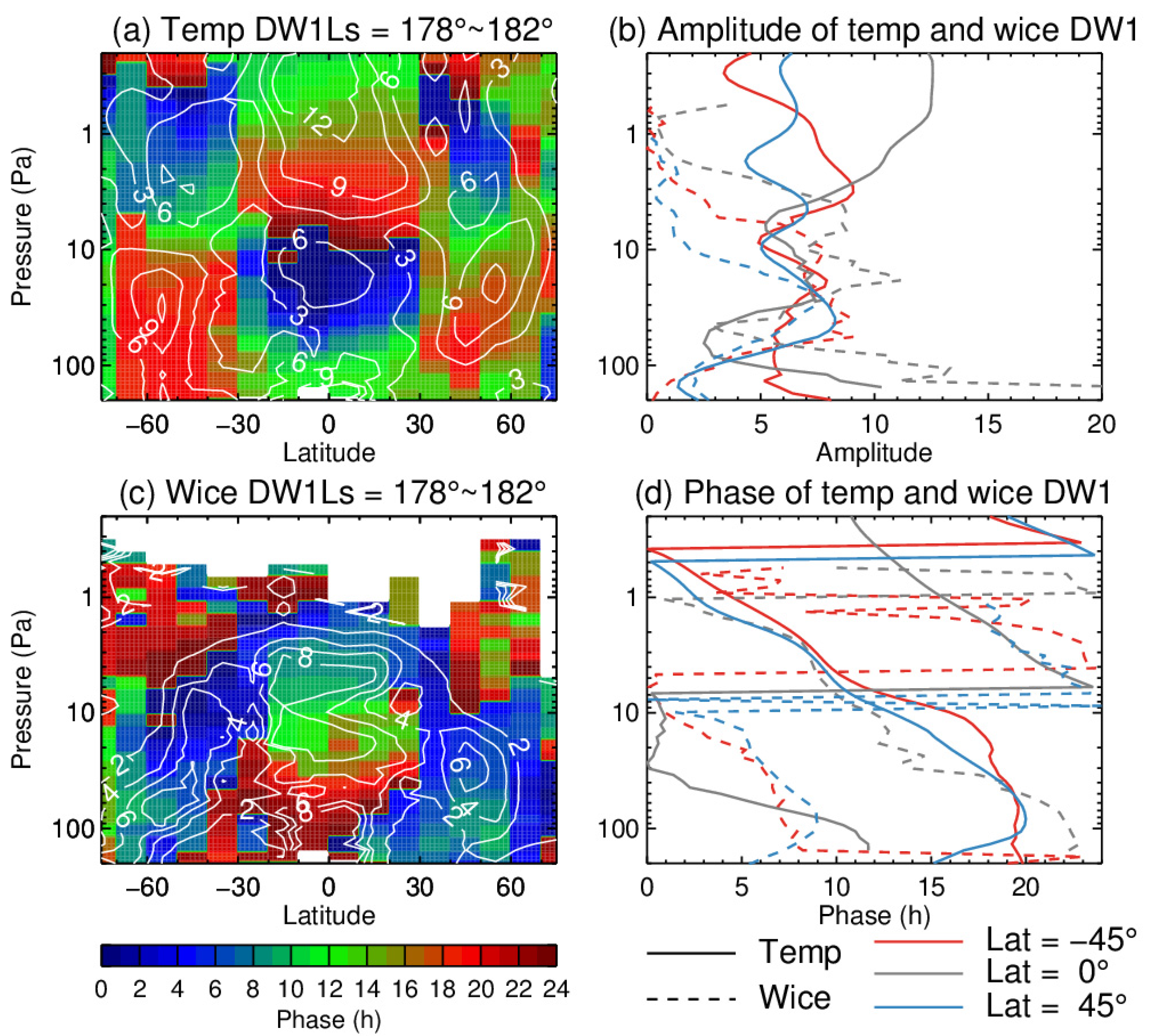
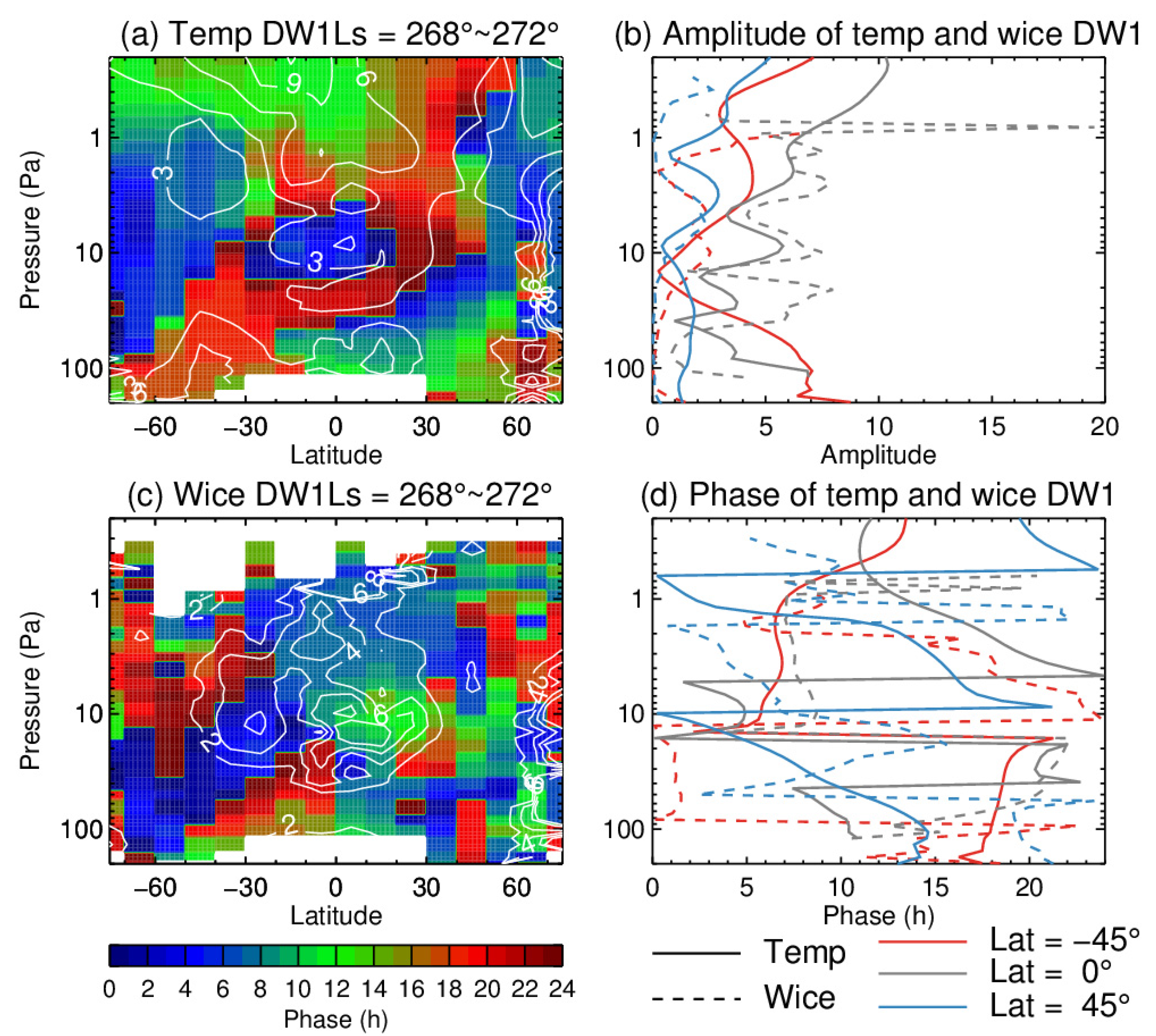
3.1. The Latitude–Altitude Structure of Temperature and Water Ice DW1

Figure 5 and Figure 6 show the latitude–altitude (pressure level) cross-section of the amplitudes and phases of the extracted temperature and water ice DW1. Several typical features are prominent and consistent with the day–night difference structures shown in Figure 3. The general structure at the fall equinox is symmetric meridionally. The temperature DW1 (diurnal tide) amplitude at low latitudes has a peak of 12 K above 1 Pa and a second peak of 8 K between 100 and 10 Pa, while at the middle latitudes of both hemispheres, it also has two layers of peaks (6–8 K), with one at ~5 Pa and the other at ~20 Pa. A latitude band centered at 30°N and 30°S of the small amplitude (less than 3 K) separates the maxima of the low and middle latitudes. Correspondingly, we can also see similar distributions in the water ice DW1 amplitude with the maxima located at low latitudes and mid-latitudes (45°N and 45°S, especially). The maximum amplitude of water ice DW1 is ~12 × 10−4, comparable to the maximum in the day–night difference field (~15 × 10−4) shown in Figure 3b, suggesting the dominant role of the DW1 component in the water ice diurnal variations.
On the other hand, both the temperature and water ice phase structures show a general downward phase progression with the height (right panels of Figure 5), corresponding to the order of the red–green–blue cycle in the upward change of the color shading (left panels of Figure 5). According to classical theory, the downward phase progression indicates an upward energy and momentum transport [44]. Another prominent feature is the half-period phase difference (12 h) between the low and middle latitudes. According to the Hough analysis, such phase reversal across latitudes in the temperature DW1 can be explained by the structure of the dominant gravity mode [36,37]. The dominant gravity mode changes signs at 30°N and 30°S so that we can see antinodes with reversal signs on the two sides. The water ice DW1 phase shares the same characteristics as the temperature DW1 but is totally out of phase by ~12 h, suggesting an accurate control of the daytime sublimation and nighttime condensation by the thermal effect of the temperature DW1 [24,25]. As for the northern winter solstice, however, the amplitude and phase structures are all distorted compared to those at the equinox. This is relevant to the significant increase of airborne dust and the induced reduction of water ice, especially during major dust storms of the dusty season, which will be discussed in the following sections.

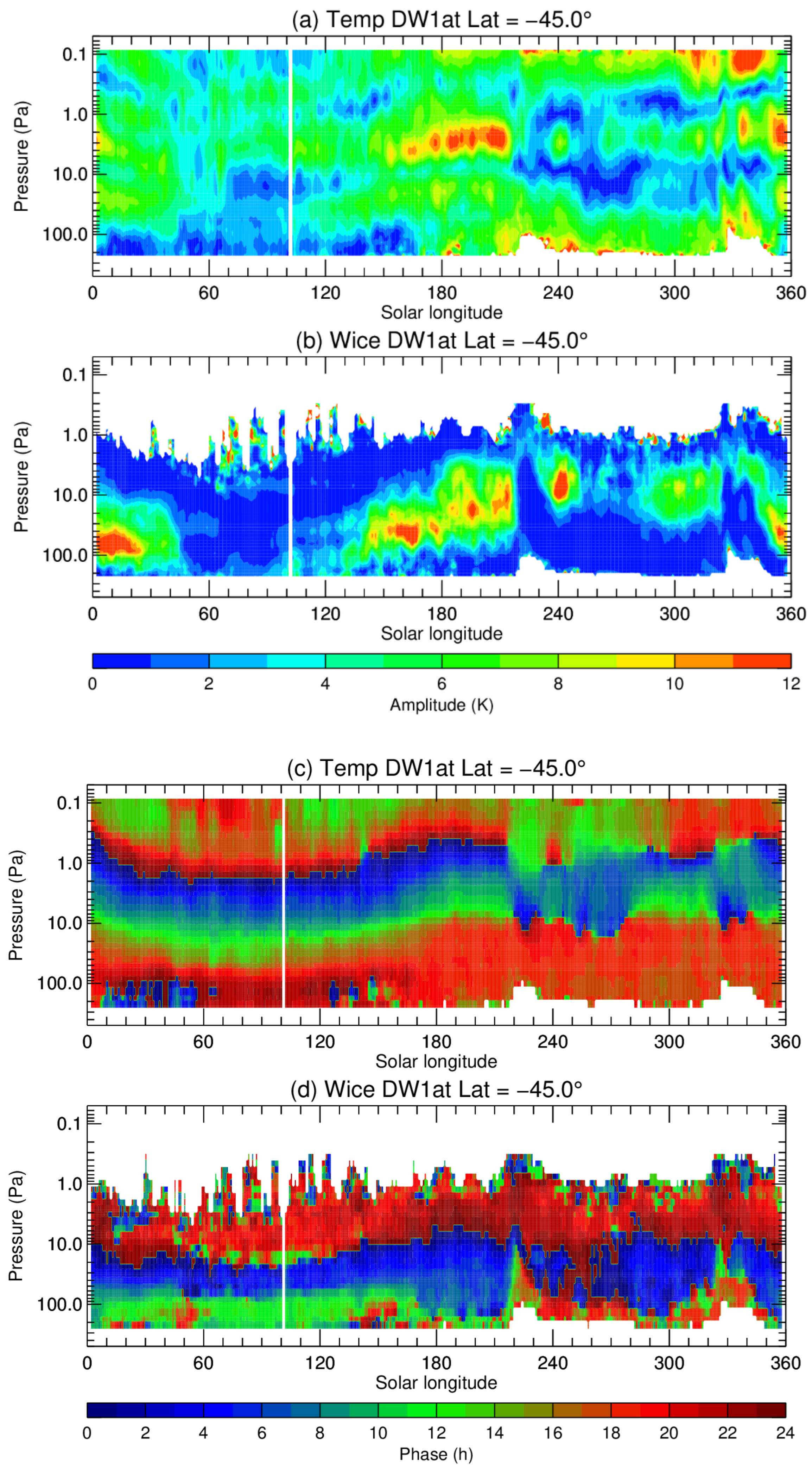
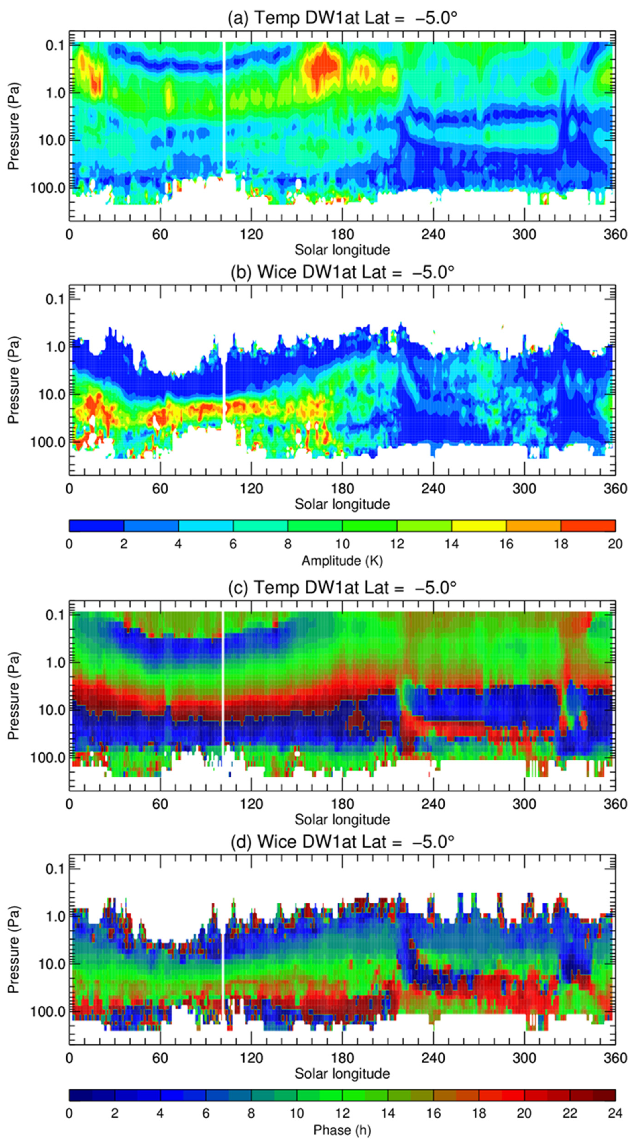
3.2. Seasonal Variations of the Temperature and Water Ice DW1

As discussed above, the DW1 peaks concentrate at the low and middle latitudes. This section chooses three typical latitudes (45°S, 5°S, and 45°N) to investigate their seasonal variations, as shown in Figure 7, Figure 8 and Figure 9. Previous studies [31] suggested that the temperature DW1 amplitude shows strong semiannual variations at low and southern middle latitudes but a weak one at northern middle latitudes. During equinoxes, the maximum amplitude reaches 12 K near 5–0.1 Pa at the equator region and 6 K/9 K near ~20/~3 Pa at the southern middle latitudes. The temperature DW1 phase also shows relatively more complicated semiannual variations if neglecting the abnormal phase structure during major dust storms [36] (the major dust storms and their occurring periods will be discussed later). In addition, the phase structure (red–green–blue color cycle) is more stretched (corresponding to longer vertical wavelengths) during the equinox than the solstice periods. This may be related to the modifications by the seasonal variations of the zonal wind structure [45]. The apparent hemispheric asymmetry in the DW1 distribution and seasonal variations is due to the topographic dichotomy. The Southern Hemisphere is 3 km higher than the Northern, on average, which may induce an asymmetric mean meridional circulation [46].
The water ice DW1, however, is more complicated during the seasonal variations. While its amplitude shows semiannual variations at the southern middle latitudes similar to the temperature DW1, those at the northern middle latitudes and equator region vary more annually, with a persistent distribution in the entire aphelion seasons from 0° to 190° Ls but a remarkable reduction in the other half of the year (Figure 8 and Figure 9). However, the case of the water ice DW1 phase is similar to that of the temperature DW1, excluding the occurring period of major dust storms. It also stretches more during the equinox than the solstice periods.

3.3. The Correlation between Water Ice and Temperature DW1

As discussed in Section 3.2, the amplitude of water ice DW1 has more complicated seasonal variations than the phase. This is partly because the amplitude is an absolute quantity related not only to the force (the diurnal tide, in this context) driving it but to the background abundance of water ice. Due to the increase of the solar radiation, the Martian lower atmosphere (below 10 Pa) during the perihelion seasons is warmer, thus increasing the sublimation of water ice. Therefore, the water ice abundance, especially at the low to middle latitudes, is higher in the aphelion seasons than in the perihelion seasons [42], resulting in a larger water ice DW1 amplitude in the first half-year. However, the DW1 phase is more of a relative quantity representing the relative change of the abundance [47]. This section quantifies their correlations by using the phase relation between the temperature and water ice DW1.
Theoretically, the water ice and temperature DW1 are accurately positively correlated for a particular pressure level if their phase difference is 0 h while anticorrelated if it is 12 h, either phase lagging or advancing. Figure 10 shows the seasonal variations of the absolute value of their phase differences at the low and middle latitudes. The phase differences are larger than 8 h (approximately anticorrelated, shown by the red color shading) at most regions during the aphelion seasons, except for the layers between 10 and 20 Pa at the middle latitudes. However, during the dusty seasons, especially in the lower atmosphere, it is out of phase or even in phase (shown by green and blue color shading). This may be due to the warmer atmosphere and intense and frequent dust activity.

4. Discussion

Diurnal variations of water ice are ubiquitous in the Martian atmosphere, as shown by the above observational results. However, their amplitude and phase structure are not always correlated with the diurnal tide (antiphase in the case of the phase relation), which is suggested to be the dominant driver by previous studies [15,24,25,37]. In this section, we discuss the possible factors behind these mismatching phenomena, such as dust activity, water ice abundance, and the amplitude of temperature DW1 that stands for the strength of the diurnal tide. To quantify their relations, we conducted statistic investigations on the occurrence frequency of antiphase events with the dust opacity, water ice opacity, and temperature DW1 amplitude. As shown in Figure 10, the temperature and water ice DW1 generally show antiphase relations in the first half-year. In contrast, most cases of phase difference less than 8 h occurred in the second half-year (approximately Ls = 190–360°). Therefore, the investigation was performed separately for the two half-years.
The statistic results are presented utilizing two-dimensional frequency distribution to evaluate the relative contributions from different factors: the temperature DW1 amplitude versus water ice opacity in Figure 11 and dust opacity in Figure 12. In the first half-year, the occurrence frequency of antiphase relation is not sensitive to both the water ice opacity and dust opacity but shows an increasing trend with the temperature DW1 amplitude (Figure 11a and Figure 12a). The same case happens with the averaged phase difference (Figure 11b and Figure 12b). The antiphase relation (phase difference larger than 8 h) persists no matter that the background water ice opacity/dust opacity is large 15 × 10−4/8 × 10−4 or small 5 × 10⁻⁴/2 × 10−4, as long as the diurnal tide amplitude is sufficiently large. It is more sensitive to the amplitude of the diurnal tide, since a larger amplitude results in larger ambient temperature variations for the water sublimation/condensation. In the second half-year, however, a peak of the occurrence frequency is prominent at the right upper corner of Figure 11c,d and the right lower corner of Figure 12c,d, respectively. This suggests that the antiphase relation is sensitive to both the water ice and dust opacity, i.e., the more water ice, the more it is anticorrelated, while the more dust, the less it is anticorrelated. It should be noted that the dust and water ice opacity themselves during the second half-year (i.e., the dusty seasons) are anticorrelated, because more dust induces more heating and warmer air favor ice sublimation [42]. Therefore, the sensitivity of the antiphase relation to water ice and dust opacity during the second half-year could be treated as affected by the same process, i.e., the dust activity.
During the dusty seasons (usually defined as seasons within Ls = 180–360° [48]), dust lifting processes on the surface increase and enhance the total dust optical depth in the atmosphere by several times [49]. In addition, three types of regional dust storms (A, B, and C) occur almost every year in the Southern Hemisphere [48]. A and C storms occur near the beginning and end of the dusty seasons, respectively, shown as the prominent peaks, especially at the middle latitudes, in Figure 13. They have similar northern responses due to the intensification of the overturning Hadley circulation [50]. B storms occur near the southern summer solstice but are more confined to the southern polar region, showing no prominent dust peak in the middle latitude (Figure 13). Though B storms have little dynamical influence on the northern atmosphere, they can still alter the water ice cloud abundance and distribution through their thermal effects [36].
The conclusions from phase relation statistics shown in Figure 11 and Figure 12 can be readily illustrated in the seasonal variations of the dust opacity and diurnal tide amplitude shown in Figure 13. We can see that the antiphase region marked by the black contour lines is complementary mainly to the high dust opacity abundance (the yellow to red color shading) region. When the dust height is relatively lower in the first half-year, the antiphase region could reach as low as 200 Pa at the middle latitudes. During the dusty seasons, when the dust height increases, the low boundary of the antiphase region also rises. Typically, during the three regional dust storms, when the lower atmospheric dust abundance is dramatically enhanced, and the water ice abundance decreases, the water ice diurnal variations within a deep pressure range from 200 to 10 Pa are out of phase with the diurnal tide, consistent with the statistic conclusions of Figure 11c,d and Figure 12c,d. Above 10 Pa, the water ice remains antiphase with the diurnal tide, consistent with the strong dawn–dusk asymmetry of the mesospheric cloud observed during major dust storms [30]. Previous studies have observed significant enhancements of the water vapor and ice at high altitudes (above 10 Pa) [36,51], providing sufficient background water reservoirs for the large amplitude of the diurnal variations.
Apart from the reduction of the lower atmospheric water ice, dust enhancement and dust storm activities could also affect and distort the global distribution of the diurnal tide, as shown in Figure 6, e.g., increase of the diurnal tide amplitude at the southern middle to high latitudes and decrease at the rest latitudes [31,52]. The amplitude shown in Figure 6b decreases to less than 3 K at the middle latitude of both hemispheres. We also show a diurnal tide amplitude less than 3 K in Figure 13 (the green dashed contours), which corresponds well to the out-of-phase region. Furthermore, this relation is also valid in the first half-year. The out-of-phase area at 10–20 Pa at both the northern and southern middle latitudes (also shown by the blue–green color shading in Figure 10) is generally accompanied by diurnal tide amplitudes less than 3 K. The above correlations and the statistic results shown in Figure 11 and Figure 12 all suggest a low threshold of the diurnal tide amplitude (2 to 3 K) for generating a relevant water ice diurnal variation, which could account for the ubiquitous water ice diurnal variations in the Martian atmosphere.

5. Conclusions

In this work, we used the temperature, water ice, and dust retrievals of MY 33 observed by the MCS multi-local time strategy to investigate the diurnal variations of water ice and its relation to the diurnal thermal tide. We quantified the water ice diurnal variations using nonlinear least square fitting by extracting the amplitude and phase, similar to the tidal analysis. Then, we conducted statistic investigations on the occurrence frequency of the antiphase between the temperature and water ice DW1 under different conditions of dust opacity, water ice opacity, and temperature DW1 amplitude. The new observational results can better constrain the Martian global climate model (MGCM) in the future, which is of great significance for understanding the entire Martian atmospheric environment and climate evolution. The main findings are summarized as below:
  • The maximum amplitude of the water ice DW1 is comparable to the maximum in the day–night difference field, suggesting the dominant role of the DW1 component in the water ice diurnal variation;
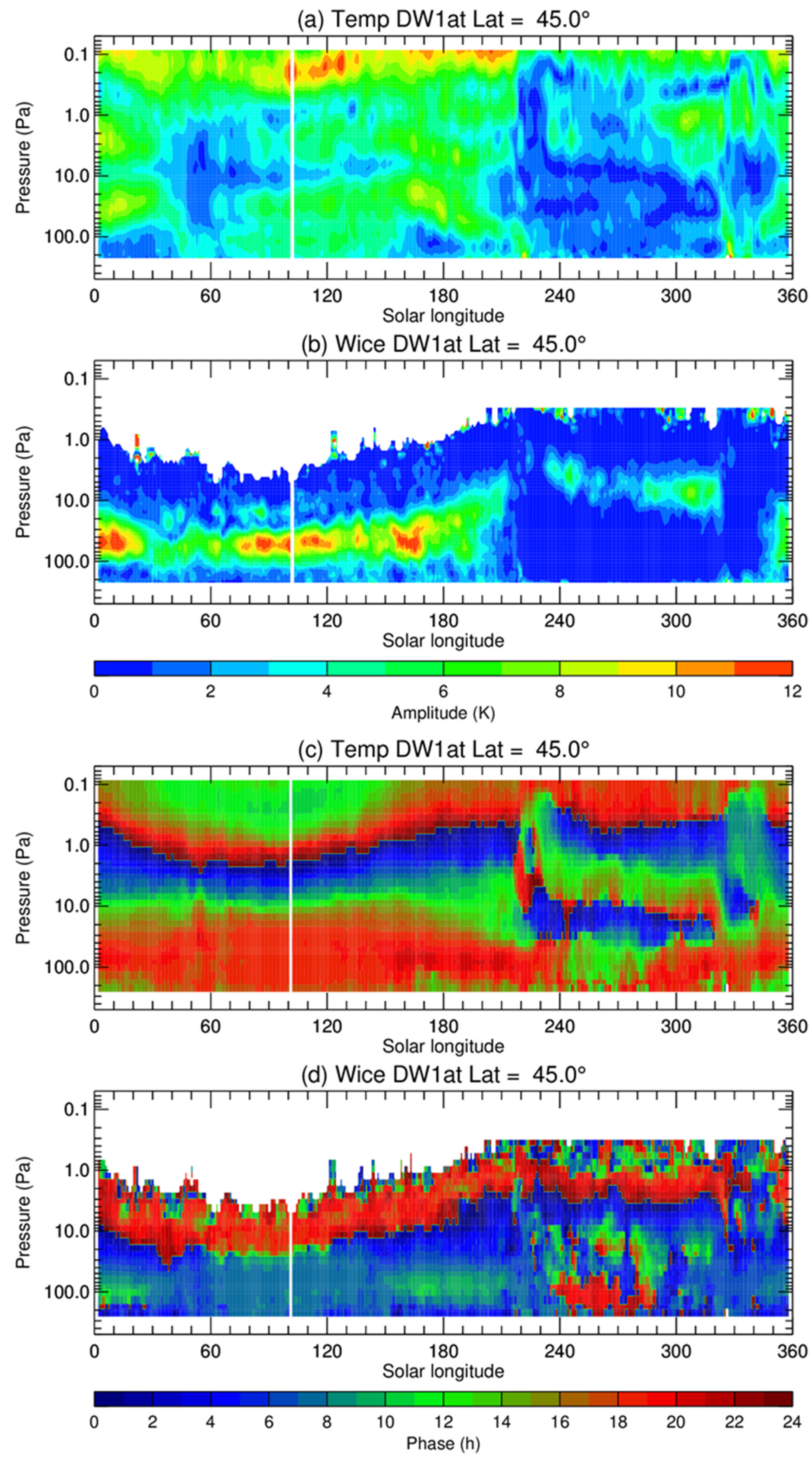
  • The water ice DW1 phase shares the same characteristics as the diurnal tide but is totally out of phase by ~12 h at the equinoxes, suggesting an accurate control of the sublimation/condensation by the thermal effect of the diurnal tide;
  • The water ice DW1 amplitude shows a semiannual variation at the southern middle latitudes similar to the temperature DW1 (diurnal tide) but that varies more annually at the northern middle latitudes and equator region, with a persistent distribution during the entire aphelion seasons from 0° to 190° Ls but a remarkable reduction in the other half-year.
  • The water ice DW1 phase generally has similar seasonal variations as the diurnal tide, with longer vertical wavelengths during the equinox compared to the solstice periods;
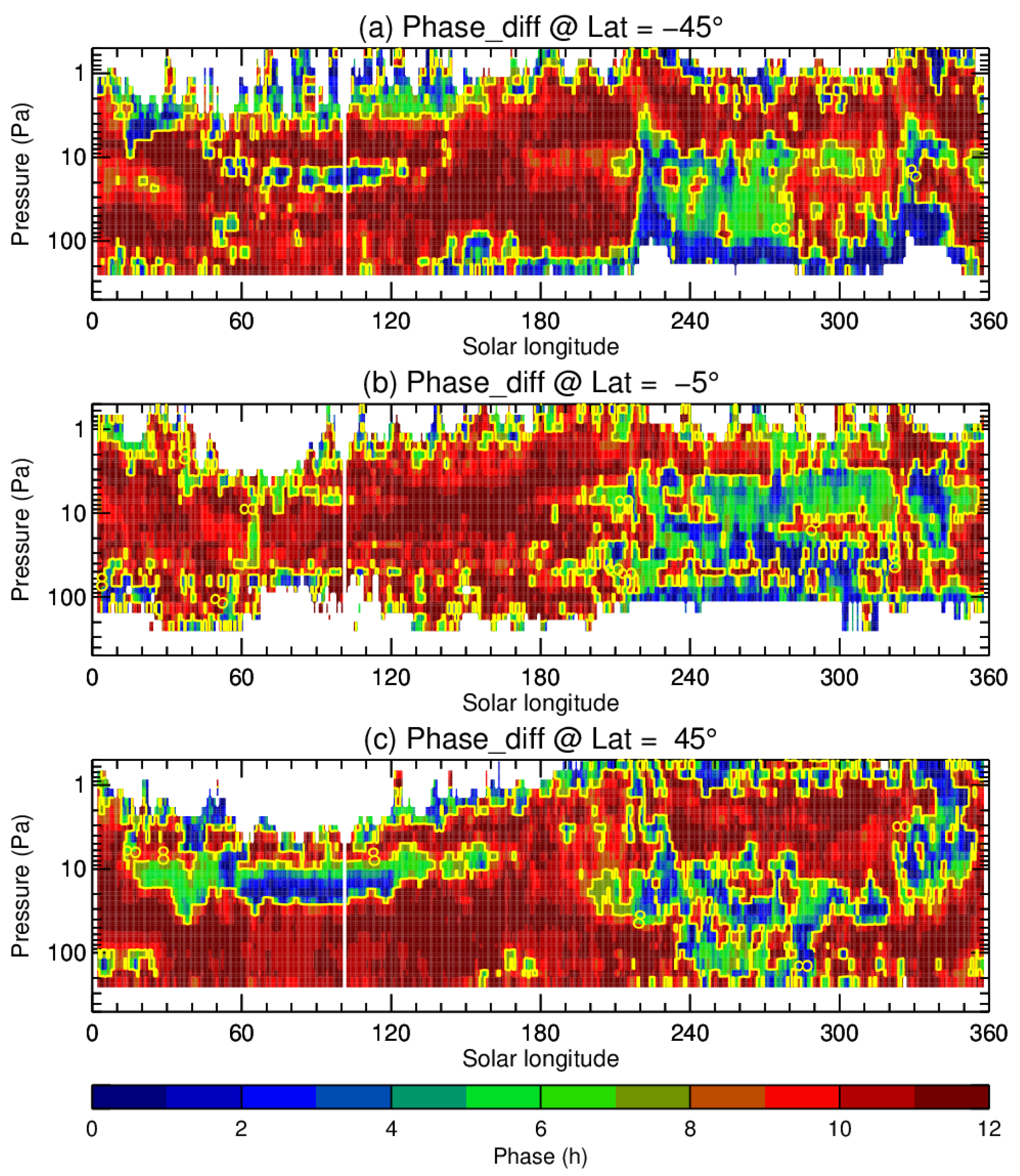
  • The quantitative statistic suggests that the temperature and water ice DW1 phase are approximately anticorrelated (defined as a phase difference greater than 8 h) at most regions during the aphelion seasons, except for the layers between 10 and 20 Pa at the middle latitudes, while it is primarily out of phase or even in phase during the dusty seasons, especially in the lower atmosphere;
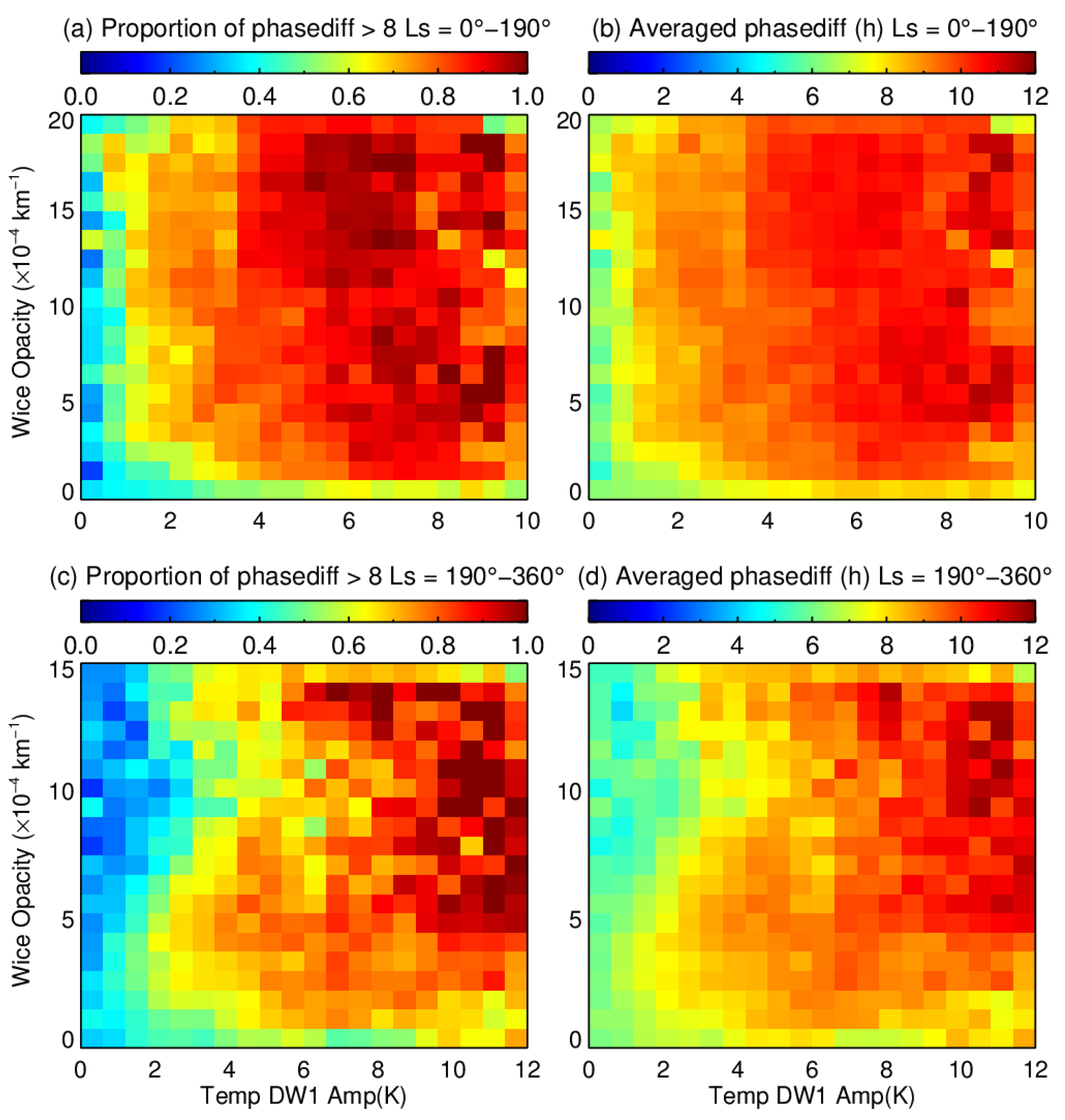
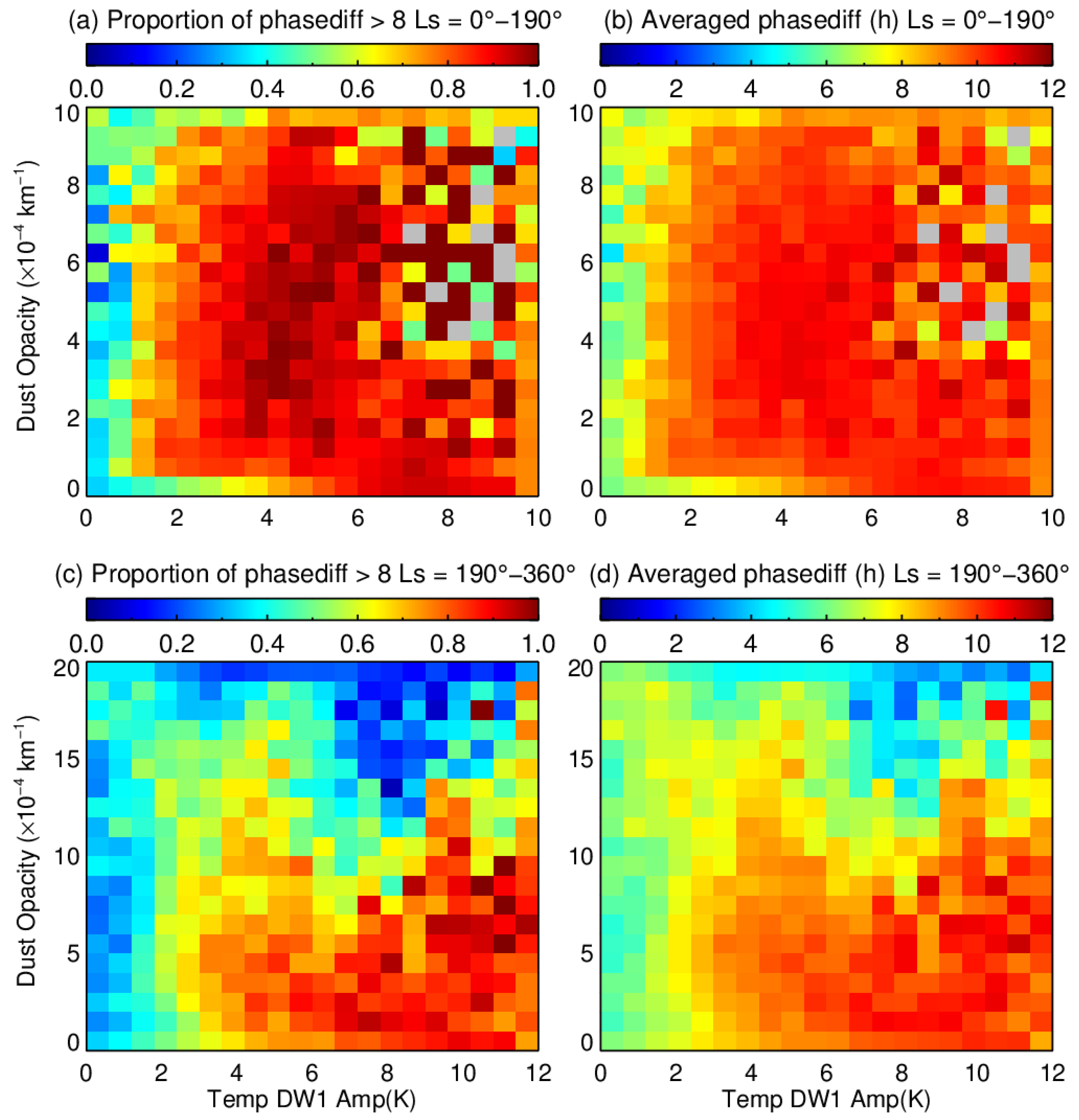
  • In the aphelion seasons, the occurrence frequency of the antiphase relation is not sensitive to both the water ice opacity and dust opacity abundance but shows an increasing trend with the temperature DW1 amplitude;
  • In the perihelion seasons, the antiphase relation is sensitive to both the water ice and dust opacity, i.e., the more water ice, the more it is anticorrelated, while the more dust, the less it is anticorrelated, both affected by the same process, i.e., the dust storm activity;
  • Finally, the statistic results suggest an unexpected low threshold of the diurnal tide amplitude (2 to 3 K) for generating a relevant water ice diurnal variation, accounting for the ubiquitous water ice diurnal variations in the Martian atmosphere.

Author Contributions

Conceptualization, Z.W. and T.L.; methodology, Z.W. and J.L.; software, Z.W. and J.L.; validation, T.L., C.Y. and J.C.; writing—original draft preparation, Z.W.; writing—review and editing and visualization, Z.W.; and supervision, T.L. All authors have read and agreed to the published version of the manuscript.

Funding

This work was supported by the B-type Strategic Priority Program of the Chinese Academy of Sciences, Grant No. XDB41000000, and the pre-research project on Civil Aerospace Technologies of China National Space Administration, Grant No. D020105. The authors also acknowledge support from the National Natural Science Foundation of China through grants 42004147 to Z.W., 42130203 to T.L., 42004133 to J.L., 41874180 to C.Y., and 41774186 to J.C.

Data Availability Statement

The MCS data presented in this study are available for download at https://pds-atmospheres.nmsu.edu/data_and_services/atmospheres_data/MARS/atmosphere_temp_prof.html (accessed on 1 May 2021).

Acknowledgments

The authors would like to thank the MCS teams for making the datasets available online.

Conflicts of Interest

The authors declare no conflict of interest.

References

  1. Leovy, C. Weather and climate on Mars. Nature 2001, 412, 245. [Google Scholar] [CrossRef]
  2. Wu, Z.; Li, T.; Heavens, N.G.; Newman, C.E.; Richardson, M.I.; Yang, C.; Li, J.; Cui, J. Earth-like thermal and dynamical coupling processes in the Martian climate system. Earth Sci. Rev. 2022, 229, 104023. [Google Scholar] [CrossRef]
  3. Yu, Z.; Cui, P.; Crassidis, J.L. Design and optimization of navigation and guidance techniques for Mars pinpoint landing: Review and prospect. Prog. Aerosp. Sci. 2017, 94, 82–94. [Google Scholar] [CrossRef]
  4. Jiang, X.; Li, S. Enabling technologies for Chinese Mars lander guidance system. Acta Astronaut. 2017, 133, 375–386. [Google Scholar] [CrossRef]
  5. Montmessin, F.; Smith, M.D.; Langevin, Y.; Mellon, M.T.; Fedorova, A. The water cycle. Atmos. Clim. Mars 2017, 18, 338. [Google Scholar]
  6. Hinson, D.P.; Wang, H.; Wilson, J.; Spiga, A. Nighttime convection in water-ice clouds at high northern latitudes on Mars. Icarus 2022, 371, 114693. [Google Scholar] [CrossRef]
  7. Steele, L.J.; Kleinböhl, A.; Kass, D.M. Observations of Ubiquitous Nighttime Temperature Inversions in Mars’ Tropics After Large-Scale Dust Storms. Geophys. Res. Lett. 2021, 48, e2021GL092651. [Google Scholar] [CrossRef]
  8. Wilson, R.J.; Guzewich, S.D. Influence of water ice clouds on nighttime tropical temperature structure as seen by the Mars Climate Sounder. Geophys. Res. Lett. 2014, 41, 3375–3381. [Google Scholar] [CrossRef]
  9. Steele, L.J.; Lewis, S.R.; Patel, M.R. The radiative impact of water ice clouds from a reanalysis of Mars Climate Sounder data. Geophys. Res. Lett. 2014, 41, 4471–4478. [Google Scholar] [CrossRef] [Green Version]
  10. Kite, E.S.; Steele, L.J.; Mischna, M.A.; Richardson, M.I. Warm early Mars surface enabled by high-altitude water ice clouds. Proc. Natl. Acad. Sci. USA 2021, 118, e2101959118. [Google Scholar] [CrossRef]
  11. Smith, M.D. Spacecraft observations of the Martian atmosphere. Annu. Rev. Earth Planet. Sci. 2008, 36, 191–219. [Google Scholar] [CrossRef] [Green Version]
  12. Guzewich, S.D.; Smith, M.D. Seasonal Variation in Martian Water Ice Cloud Particle Size. J. Geophys. Res. Planets 2019, 124, 636–643. [Google Scholar] [CrossRef] [Green Version]
  13. Guzewich, S.D.; Smith, M.D.; Wolff, M.J. The vertical distribution of Martian aerosol particle size. J. Geophys. Res. Planets 2014, 119, 2694–2708. [Google Scholar] [CrossRef]
  14. Smith, M.D.; Bandfield, J.; Christensen, P.R.; Richardson, M.I. Thermal Emission Imaging System (THEMIS) infrared observations of atmospheric dust and water ice cloud optical depth. J. Geophys. Res. Earth Surf. 2003, 108. [Google Scholar] [CrossRef] [Green Version]
  15. Hinson, D.P.; Wilson, R.J. Temperature inversions, thermal tides, and water ice clouds in the Martian tropics. J. Geophys Res. Planet 2004, 109, E1. [Google Scholar] [CrossRef]
  16. Smith, M.D.; Wolff, M.J.; Clancy, R.T.; Kleinböhl, A.; Murchie, S.L. Vertical distribution of dust and water ice aerosols from CRISM limb-geometry observations. J. Geophys. Res. Planets 2013, 118, 321–334. [Google Scholar] [CrossRef] [Green Version]
  17. Kleinböhl, A.; Schofield, J.T.; Kass, D.M.; Abdou, W.A.; Backus, C.R.; Sen, B.; Shirley, J.H.; Lawson, W.G.; Richardson, M.I.; Taylor, F.W.; et al. Mars Climate Sounder limb profile retrieval of atmospheric temperature, pressure, and dust and water ice opacity. J. Geophys. Res. Planets 2009, 114, 006. [Google Scholar] [CrossRef]
  18. Maltagliati, L.; Titov, D.V.; Encrenaz, T.; Melchiorri, R.; Forget, F.; Garcia-Comas, M.; Keller, H.U.; Langevin, Y.; Bibring, J.-P. Observations of atmospheric water vapor above the Tharsis volcanoes on Mars with the OMEGA/MEx imaging spectrometer. Icarus 2008, 194, 53–64. [Google Scholar] [CrossRef]
  19. Madeleine, J.B.; Forget, F.; Spiga, A.; Wolff, M.J.; Montmessin, F.; Vincendon, M.; Jouglet, D.; Gondet, B.; Bibring, J.P.; Langevin, Y.; et al. Aphelion water-ice cloud mapping and property retrieval using the OMEGA imaging spectrometer onboard Mars Express. J. Geophys. Res. 2012, 117, E11. [Google Scholar] [CrossRef] [Green Version]
  20. Olsen, K.S.; Forget, F.; Madeleine, J.B.; Szantai, A.; Audouard, J.; Geminale, A.; Altieri, F.; Bellucci, G.; Oliva, F.; Montabone, L.; et al. Retrieval of the water ice column and physical properties of water-ice clouds in the martian atmosphere using the OMEGA imaging spectrometer. Icarus 2021, 353, 113229. [Google Scholar] [CrossRef]
  21. Smith, M.D.; Daerden, F.; Neary, L.; Khayat, A. The climatology of carbon monoxide and water vapor on Mars as observed by CRISM and modeled by the GEM-Mars general circulation model. Icarus 2018, 301, 117–131. [Google Scholar] [CrossRef]
  22. Heavens, N.G.; Benson, J.L.; Kass, D.M.; Kleinbohl, A.; Abdou, W.A.; McCleese, D.J.; Richardson, M.I.; Schofield, J.T.; Shirley, J.H.; Wolkenberg, P.M. Water ice clouds over the Martian tropics during northern summer. Geophys. Res. Lett. 2010, 37, L18202. [Google Scholar] [CrossRef]
  23. Guha, B.K.; Panda, J.; Wu, Z. Observation of aphelion cloud belt over Martian tropics, its evolution, and associated dust distribution from MCS data. Adv. Space Res. 2021, 67, 1392–1411. [Google Scholar] [CrossRef]
  24. Benson, J.L.; Kass, D.M.; Kleinböhl, A. Mars’ north polar hood as observed by the Mars Climate Sounder. J. Geophys. Res. Planets 2011, 116, E3. [Google Scholar] [CrossRef]
  25. Benson, J.L.; Kass, D.M.; Kleinböhl, A.; McCleese, D.J.; Schofield, J.T.; Taylor, F.W. Mars’ south polar hood as observed by the Mars Climate Sounder. J. Geophys. Res. Planets 2010, 115, E12. [Google Scholar] [CrossRef]
  26. Michelangeli, D.V.; Toon, O.B.; Haberle, R.M.; Pollack, J.B. Numerical simulations of the formation and evolution of water ice clouds in the Martian atmosphere. Icarus 1993, 102, 261–285. [Google Scholar] [CrossRef]
  27. Richardson, M.I.; John, W.R.; Rodin, A.V. Water ice clouds in the Martian atmosphere: General circulation model experiments with a simple cloud scheme. J. Geophys. Res. Planets 2002, 107, E9. [Google Scholar] [CrossRef] [Green Version]
  28. Shaposhnikov, D.S.; Medvedev, A.S.; Rodin, A.V.; Yiğit, E.; Hartogh, P. Martian Dust Storms and Gravity Waves: Disentangling Water Transport to the Upper Atmosphere. J. Geophys. Res. Planets 2022, 127, e2021JE007102. [Google Scholar] [CrossRef]
  29. Chaffin, M.S.; Kass, D.M.; Aoki, S.; Fedorova, A.A.; Deighan, J.; Connour, K.; Heavens, N.G.; Kleinböhl, A.; Jain, S.K.; Chaufray, J.Y.; et al. Martian water loss to space enhanced by regional dust storms. Nat. Astron. 2021, 5, 1036–1042. [Google Scholar] [CrossRef]
  30. Liuzzi, G.; Villanueva, G.L.; Crismani, M.M.J.; Smith, M.D.; Mumma, M.J.; Daerden, F.; Aoki, S.; Vandaele, A.C.; Clancy, R.T.; Erwin, J.; et al. Strong Variability of Martian Water Ice Clouds During Dust Storms Revealed From ExoMars Trace Gas Orbiter/NOMAD. J. Geophys. Res. Planets 2020, 125, e2019JE006250. [Google Scholar] [CrossRef]
  31. Wu, Z.; Li, T.; Zhang, X.; Li, J.; Cui, J. Dust tides and rapid meridional motions in the Martian atmosphere during major dust storms. Nat. Commun. 2020, 11, 614. [Google Scholar] [CrossRef] [PubMed] [Green Version]
  32. Shaposhnikov, D.S.; Medvedev, A.S.; Rodin, A.V.; Hartogh, P. Seasonal Water “Pump” in the Atmosphere of Mars: Vertical Transport to the Thermosphere. Geophys. Res. Lett. 2019, 46, 4161–4169. [Google Scholar] [CrossRef] [Green Version]
  33. Forbes, J.M. Tidal and planetary waves. In The Upper Mesosphere and Lower Thermosphere: A Review of Experiment and Theory; Geophysical Monograph Series; AGU: Washington, DC, USA, 1995; Volume 87, pp. 67–87. [Google Scholar]
  34. Wu, Z.; Li, J.; Li, T.; Cui, J. The dust storm and its interaction with atmospheric waves on Mars. Rev. Geophys. Planet. Phys. 2021, 52, 402. [Google Scholar] [CrossRef]
  35. Forbes, J.M.; Zhang, X.L.; Forget, F.; Millour, E.; Kleinbohl, A. Solar Tides in the Middle and Upper Atmosphere of Mars. J. Geophys Res. Space 2020, 125, e2020JA028140. [Google Scholar] [CrossRef]
  36. Wu, Z.; Li, T.; Li, J.; Zhang, X.; Yang, C.; Cui, J. Abnormal Phase Structure of Thermal Tides During Major Dust Storms on Mars: Implications for the Excitation Source of High-altitude Water Ice Clouds. J. Geophys. Res. Planets 2021, 126, e2020JE006758. [Google Scholar] [CrossRef]
  37. Lee, C.; Lawson, W.G.; Richardson, M.I.; Heavens, N.G.; Kleinböhl, A.; Banfield, D.; McCleese, D.J.; Zurek, R.; Kass, D.M.; Schofield, J.T.; et al. Thermal tides in the Martian middle atmosphere as seen by the Mars Climate Sounder. J. Geophys. Res. 2009, 114, E03005. [Google Scholar] [CrossRef]
  38. Wu, Z.; Li, T.; Dou, X. Seasonal variation of Martian middle atmosphere tides observed by the Mars Climate Sounder. J. Geophys. Res. Planets 2015, 120, 2206–2223. [Google Scholar] [CrossRef] [Green Version]
  39. Kleinböhl, A.; Spiga, A.; Kass, D.M.; Shirley, J.H.; Millour, E.; Montabone, L.; Forget, F. Diurnal variations of dust during the 2018 global dust storm observed by the Mars Climate Sounder. J. Geophys. Res. Planets 2020, 125, e2019JE006115. [Google Scholar] [CrossRef] [Green Version]
  40. McCleese, D.J.; Schofield, J.T.; Taylor, F.W.; Calcutt, S.B.; Foote, M.C.; Kass, D.M.; Leovy, C.B.; Paige, D.A.; Read, P.L.; Zurek, R.W. Mars Climate Sounder: An investigation of thermal and water vapor structure, dust and condensate distributions in the atmosphere, and energy balance of the polar regions. J. Geophys. Res. 2007, 112, E05S06. [Google Scholar] [CrossRef] [Green Version]
  41. Kleinböhl, A.; John Wilson, R.; Kass, D.M.; Schofield, J.T.; McCleese, D.J. The semidiurnal tide in the middle atmosphere of Mars. Geophys. Res. Lett. 2013, 40, 1952–1959. [Google Scholar] [CrossRef]
  42. McCleese, D.J.; Heavens, N.G.; Schofield, J.T.; Abdou, W.A.; Bandfield, J.L.; Calcutt, S.B.; Irwin, P.G.J.; Kass, D.M.; Kleinböhl, A.; Lewis, S.R.; et al. Structure and dynamics of the Martian lower and middle atmosphere as observed by the Mars Climate Sounder: Seasonal variations in zonal mean temperature, dust, and water ice aerosols. J. Geophys. Res. 2010, 115, E5. [Google Scholar] [CrossRef]
  43. McCleese, D.J.; Schofield, J.T.; Taylor, F.W.; Abdou, W.A.; Aharonson, O.; Banfield, D.; Calcutt, S.B.; Heavens, N.G.; Irwin, P.G.J.; Kass, D.M.; et al. Intense polar temperature inversion in the middle atmosphere on Mars. Nat. Geosci. 2008, 1, 745–749. [Google Scholar] [CrossRef]
  44. Chapman, S.; Lindzen, R.S. Atmospheric Tides; D. Reidel: Dordrecht, The Netherlands, 1970; 200p. [Google Scholar]
  45. Wu, Z.; Li, T.; Dou, X. What causes seasonal variation of migrating diurnal tide observed by the Mars Climate Sounder? J. Geophys. Res. Planets 2017, 122, 1227–1242. [Google Scholar] [CrossRef]
  46. Richardson, M.I.; Wilson, R.J. A topographically forced asymmetry in the martian circulation and climate. Nature 2002, 416, 298–301. [Google Scholar] [CrossRef]
  47. Li, J.; Wu, Z.; Li, T.; Zhang, X.; Cui, J. The diurnal transport of atmospheric water vapor during major dust storms on Mars based on the Mars Climate Database, version 5.3. Earth Planet. Phys. 2020, 4, 550–564. [Google Scholar] [CrossRef]
  48. Kass, D.M.; Kleinböhl, A.; McCleese, D.; Schofield, J.; Smith, M. Interannual similarity in the Martian atmosphere during the dust storm season. Geophys. Res. Lett. 2016, 43, 6111–6118. [Google Scholar] [CrossRef]
  49. Montabone, L.; Forget, F.; Millour, E.; Wilson, R.J.; Lewis, S.R.; Cantor, B.; Kass, D.M.; Klembohl, A.; Lemmon, M.T.; Smith, M.D.; et al. Eight-year climatology of dust optical depth on Mars. Icarus 2015, 251, 65–95. [Google Scholar] [CrossRef] [Green Version]
  50. Wilson, R.J. Martian Dust Storms, Thermal Tides, and the Hadley Circulation. Lpi Contrib. 2012, 1675, 8069. [Google Scholar]
  51. Heavens, N.G.; Kleinbohl, A.; Chaffin, M.S.; Halekas, J.S.; Kass, D.M.; Hayne, P.O.; McCleese, D.J.; Piqueux, S.; Shirley, J.H.; Schofield, J.T. Hydrogen escape from Mars enhanced by deep convection in dust storms. Nat. Astron. 2018, 2, 126–132. [Google Scholar] [CrossRef]
  52. Banfield, D.; Conrath, B.; Pearl, J.C.; Smith, M.D.; Christensen, P. Thermal tides and stationary waves on Mars as revealed by Mars Global Surveyor thermal emission spectrometer. J. Geophys. Res. Planet 2000, 105, 9521–9537. [Google Scholar] [CrossRef]
Figure 1. Latitude and local time coverage of the MCS observation. The blue boxes indicate the “in-track” observations in one orbit of MRO. The grey boxes indicate the multi-local time observational strategy, including the “cross-track” and “off-track” observations [40,41]. The blue horizontal dash lines show the latitude bin boundaries, while the red vertical dash lines show the local time bin boundaries of the data binning strategy used in this work.
Remotesensing 14 02235 g001
Figure 2. The zonal mean nighttime (a,c) and daytime (b,d) MCS temperature (a,b) and water ice (c,d) retrievals at the northern fall equinox (Ls = 180° and 5° averaged). The black contours in each panel indicate the data uncertainty.
Remotesensing 14 02235 g002
Figure 3. The differences between 3 p.m. and 3 a.m. in the temperature (a,c) and water ice opacity (b,d) at the northern fall equinox (a,b) and northern winter solstice (c,d).
Remotesensing 14 02235 g003
Figure 4. An example of 8-sol time evolutions of the zonal mean temperature (color shading) and water ice opacity (dashed contours) at (a) the northern and (b) southern middle latitudes during the northern fall equinox. All data are obtained by the MCS cross-track observational strategy to increase the local time coverage (Figure 1). The vertical grey dotted lines indicate the data sampling local time. The 0 a.m. of each sol corresponds to the marking place of the x coordinate value. Note that the water opacity value has been multiplied by 104.
Remotesensing 14 02235 g004
Figure 5. Latitude–altitude structures of (a) the temperature and (c) water ice DW1 amplitude (white contours) and phase (color shading) at the northern fall equinox. (b,d) The comparisons of their amplitude and phase, respectively, at the southern and northern middle latitudes and the equator region. The solid and dashed lines in (b,d) indicate the temperature and water ice DW1, respectively, while the colors represent different latitudes. Note that the water opacity value has been multiplied by 104.
Remotesensing 14 02235 g005
Figure 6. Latitude–altitude structures of (a) the temperature and (c) water ice DW1 amplitude (white contours) and phase (color shading) at the northern winter solstice. (b,d) The comparisons of their amplitude and phase, respectively, at the southern and northern middle latitudes and the equator region. The solid and dashed lines in (b,d) indicate the temperature and water ice DW1, respectively, while the colors represent different latitudes. Note that the water opacity value has been multiplied by 104.
Remotesensing 14 02235 g006
Figure 7. Seasonal variations of the temperature (a,c) and water ice (b,d) DW1 amplitude (a,b) and phase (c,d) at 45°S. Note that the water opacity value has been multiplied by 104.
Remotesensing 14 02235 g007
Figure 8. Seasonal variations of the temperature (a,c) and water ice (b,d) DW1 amplitude (a,b) and phase (c,d) at 5°S. Note that the water opacity value has been multiplied by 104.
Remotesensing 14 02235 g008
Figure 9. Seasonal variations of the temperature (a,c) and water ice (b,d) DW1 amplitude (a,b) and phase (c,d) at 45°N. Note that the water opacity value has been multiplied by 104.
Remotesensing 14 02235 g009
Figure 10. Seasonal variations of the absolute phase differences between the temperature and water ice DW1 at (a) 45°S, (b) 5°S, and (c) 45°N. The gold contours indicate a phase difference of 8 h.
Remotesensing 14 02235 g010
Figure 11. Occurrence frequency of the phase differences larger than 8 h (approximately anticorrelated) with the temperature DW1 amplitude (x-axis) and daily mean water ice abundance (y-axis). The statistic includes data of all latitudes from 75°S to 75°N and pressure levels from 200 to 1 Pa during (a) Ls = 0°–190° and (b) Ls = 190°–360°. (b,d) The mean phase difference values corresponding to (a,c), respectively.
Remotesensing 14 02235 g011
Figure 12. Occurrence frequency of the phase differences larger than 8 h (approximately anticorrelated) with the temperature DW1 amplitude (x-axis) and daily mean dust abundance (y-axis). The statistic includes data of all latitudes from 75°S to 75°N and pressure levels from 200 to 1 Pa during (a) Ls = 0°–190° and (b) Ls = 190°–360°. (b,d) The mean phase difference values corresponding to (a,c), respectively. The grey boxes indicate 0 events.
Remotesensing 14 02235 g012
Figure 13. Seasonal variations of the zonal mean dust opacity at (a) 45°S, (b) 5°S, and (c) 45°N. The black contours indicate a phase difference of 8 h, as shown in Figure 10. The green dashed contours indicate a temperature DW1 amplitude that is less than 3 K. The three regional dust storms of MY 33 and their approximate duration periods [36] are, respectively: A storm, Ls = 218°–236°; B storm, Ls = 250°–285°; and C storm, Ls = 325°–345°.
Remotesensing 14 02235 g013
Publisher’s Note: MDPI stays neutral with regard to jurisdictional claims in published maps and institutional affiliations.

