Abstract
The long-time coherent integration can effectively improve the detection ability of radar targets. However, this strategy usually shows poor effect in resisting the sea clutter, which produces difficulties for accurate estimation of sea clutter characteristics and results in the inability to differentiate between the target and sea clutter. To solve this problem, a two-stage method is proposed, which consists of the sea clutter suppression stage and target decision stage. In the sea clutter suppression stage, the correlation time differences in the time and the space domains are adopted to estimate the correlation of sea clutter. Then, a selective whitening filter is proposed, which is performed more adaptively according to the estimation results. In the decision stage, the peak average ratio in the fractional Fourier domain (FRFT-PAR) is presented, which can make better use of the energy accumulation characteristics and further suppress the interference of sea clutter. Experiments on the IPIX datasets with various observation times and polarization modes are included. The results indicate that the proposed method could not only effectively suppress sea clutter but also achieve better target detection performance than baseline algorithms.
1. Introduction
The detection of low-reflection and slow speed small radar target (LSS-target) plays an important role in target detection due to military and commercial needs [1,2]. However, detecting the LSS-target in concentrated sea clutter is a big challenge. Because the characteristics of complex sea clutter are affected by terrain and weather, the target echoes usually have a low signal to noise ratio (SNR). Traditional methods [3,4,5] usually have low detection probability and high false alarm because their detection abilities are easily interfered with by sea clutter of different densities. With the development of the radar theory, more and more studies are being conducted on the characteristics of sea clutter. Therefore, it is important to perform sea clutter suppression based on refined characteristics in radar target detection.
The long-time coherent integration strategy [6,7,8,9] has been widely applied in recent studies because it is a feasible way to accumulate energy from multiple echoes and contributes to improving the SNR of target echoes. Nevertheless, the target moves with the undulating waves. The effect of the across-range unit (ARU) and phase modulations cannot be ignored [10], which would limit the improvement of detection performance. Then, the Radon–Fourier transform (RFT) [11] and the Radon–Fractional–Fourier transform (RFRFT) [12] are presented. They overcome the ARU effect and phase modulations by jointly searching along with the range and velocity directions of moving targets. However, the surge of sea clutter usually lasts for seconds with a certain movement pattern, and its energy would also be accumulated. Therefore, the long-time coherent integration-based methods cannot effectively overcome the interference of sea clutter.
In the meanwhile, due to the existence of multifractal behaviors of sea clutter [13,14], the fractal features in the Fractional–Fourier transform (FRFT) domain [15] are used to identify sea clutter and target. However, the estimation accuracy of fractal features largely depends on the observation time. It would be higher with the extension of the observation time when the observation time is within a certain range. In addition, extracting the fractal features requires a huge computational cost.
The correlation analysis, which utilizes the stationarity difference, is another way to distinguish between sea clutter and target. The adaptive normalized matching filter (ANMF) [16,17] uses the referenced samples to directly estimate the covariance matrix. It is a very effective detector when the sea clutter is approximately stationary during the observation time. However, when the observation time is long, its detection performance will drop a lot and will be disturbed by the Doppler spread. To address this issue, a combined adaptive normalized matching filter (CANMF) [18,19] is proposed, which supposes that the Doppler spread and range walk across bins can be ignored when the long integration duration is divided into several disjoint subintervals. In this way, a series of ANMF with different normalized Doppler frequencies constitutes the CANMF, which helps to estimate the characteristics of sea clutter more accurately. Besides, the time-frequency method is introduced in the S-method [20,21], which realizes the time-frequency representation and decomposition by utilizing the autocorrelation of the target echoes. The detection statistics are extracted from the decomposed components to separate the target from the sea clutter. However, the detection performances of methods based on autocorrelation are often disturbed by spatial changes. To solve this problem, the cross S-method (CSM) [22,23] realizes the signal decomposition by jointly combining two adjacent bins. It uses the signal synthesis method to decompose the joint time-space-frequency representation, which guarantees the ability to detect range-spread targets without correcting the range migration. Nevertheless, in the case of joint time-space-frequency representation, more sea clutter components will inevitably be mixed into the decomposed components, and the improvement of detection performance is also limited. Besides, the above methods rely on the estimation of reference bins. If there are not enough ideal reference bins available, the interference of sea clutter will remain.
A two-stage method is proposed in this paper to solve these problems, which consists of the sea clutter suppression stage and the target decision stage. In the sea clutter suppression stage, the correlation time differences in the time domain and space domain are adopted to estimate the correlation of sea clutter. According to the estimation results, the sea clutter in different range bins is suppressed. After that, a selective whitening filter is presented, which is performed more adaptively according to the estimation results and facilitates the suppression of the sea clutter in the echo components. In the decision stage, the peak average ratio in the fractional Fourier domain (FRFT-PAR) is presented, which is adopted to make better use of the energy accumulation characteristics and further suppress the interference of sea clutter. The main contributions of this paper can be summarized as follows:
- (1)
- A correlation estimation method of sea clutter based on correlation time is proposed. The correlation of sea clutter is evaluated by calculating the correlation time in both time and space domains. According to the estimation results, the sea clutter in different range bins is suppressed.
- (2)
- A selective whitening filter is proposed. In the selective whitening filter, the processing bins are selected adaptively according to the sea clutter correlation estimation results, which can facilitate the suppression of the sea clutter in the target echo components and reduce the computational load.
- (3)
- The FRFT-PAR is presented to distinguish between the sea clutter and target, which is adopted to make better use of the energy accumulation characteristics and further suppress the interference of sea clutter.
2. Material and Methods
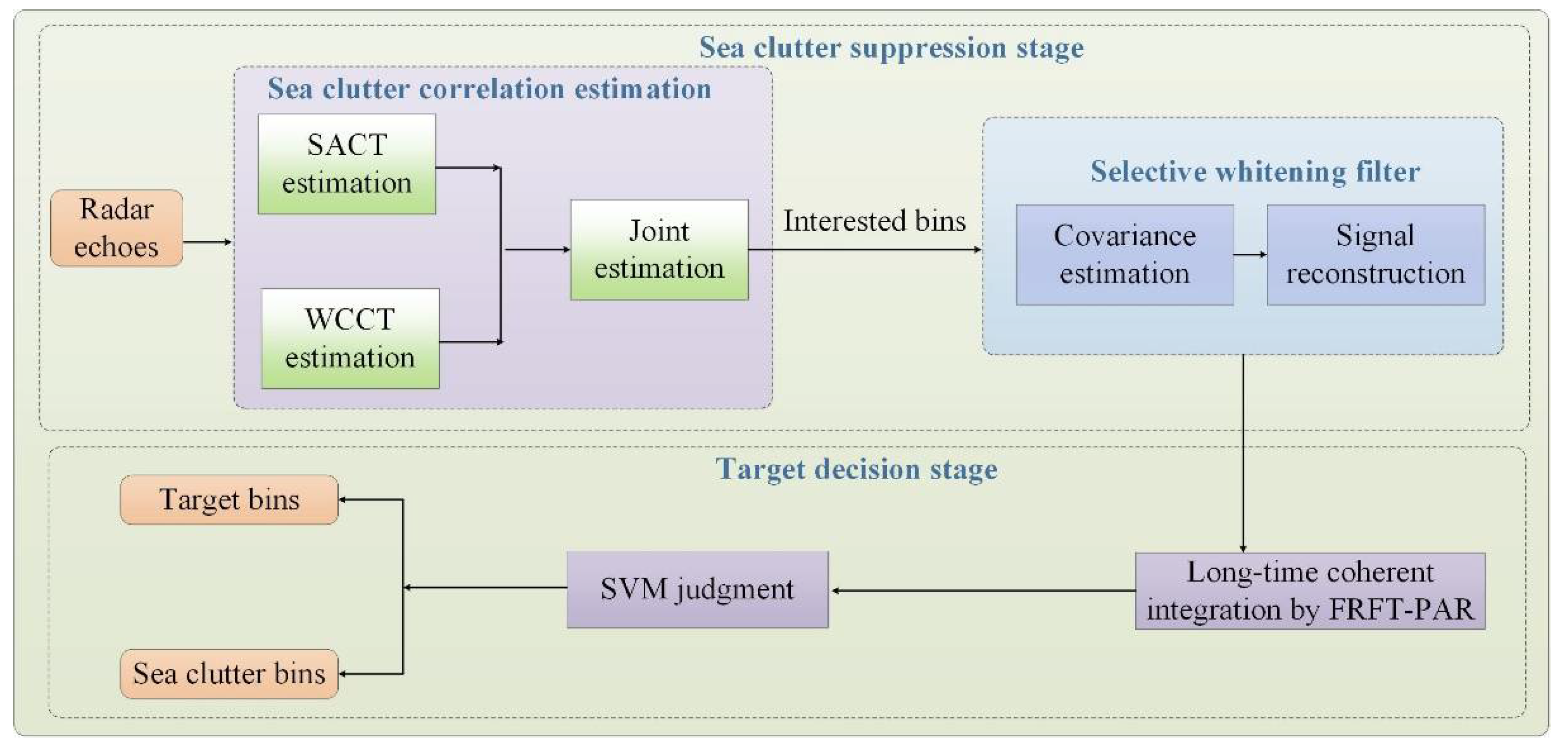
The overall architecture of the proposed algorithm is illustrated in Figure 1. The core goal of this algorithm is to suppress sea clutter more effectively by using the correlation characteristics of sea clutter. For this reason, a two-stage method based on sea clutter correlation estimation is designed. It consists of two successive stages: the sea clutter suppression stage and the target decision stage. In the sea clutter suppression stage, the strong auto-correlation time (SACT) in the time domain and the weak cross-correlation time (WCCT) in the space domain are adopted to estimate the correlation between sea clutter. Then, the selective whitening filter is performed according to the correlation estimation results of interested bins. In the target decision stage, the FRFT-PAR is presented, and a judgment model is built by SVM tools. The model is then adopted to distinguish between the target and sea clutter in the interested range bins.

Figure 1.
Flow chart of the proposed algorithm.
2.1. Sea Clutter Suppression Stage
In the maritime environment, the detection of low observable radar target can be described by the following binary hypothesis testing [18,24]:
where represents the echoes received by a certain range bin, represents the pure sea clutter, and represents the target echoes. If the hypothesis is accepted, then and denotes the pure sea clutter. Otherwise, the hypothesis is accepted, denotes the echoes of the target bin, and the echoes are the mix of target echoes and sea clutter.
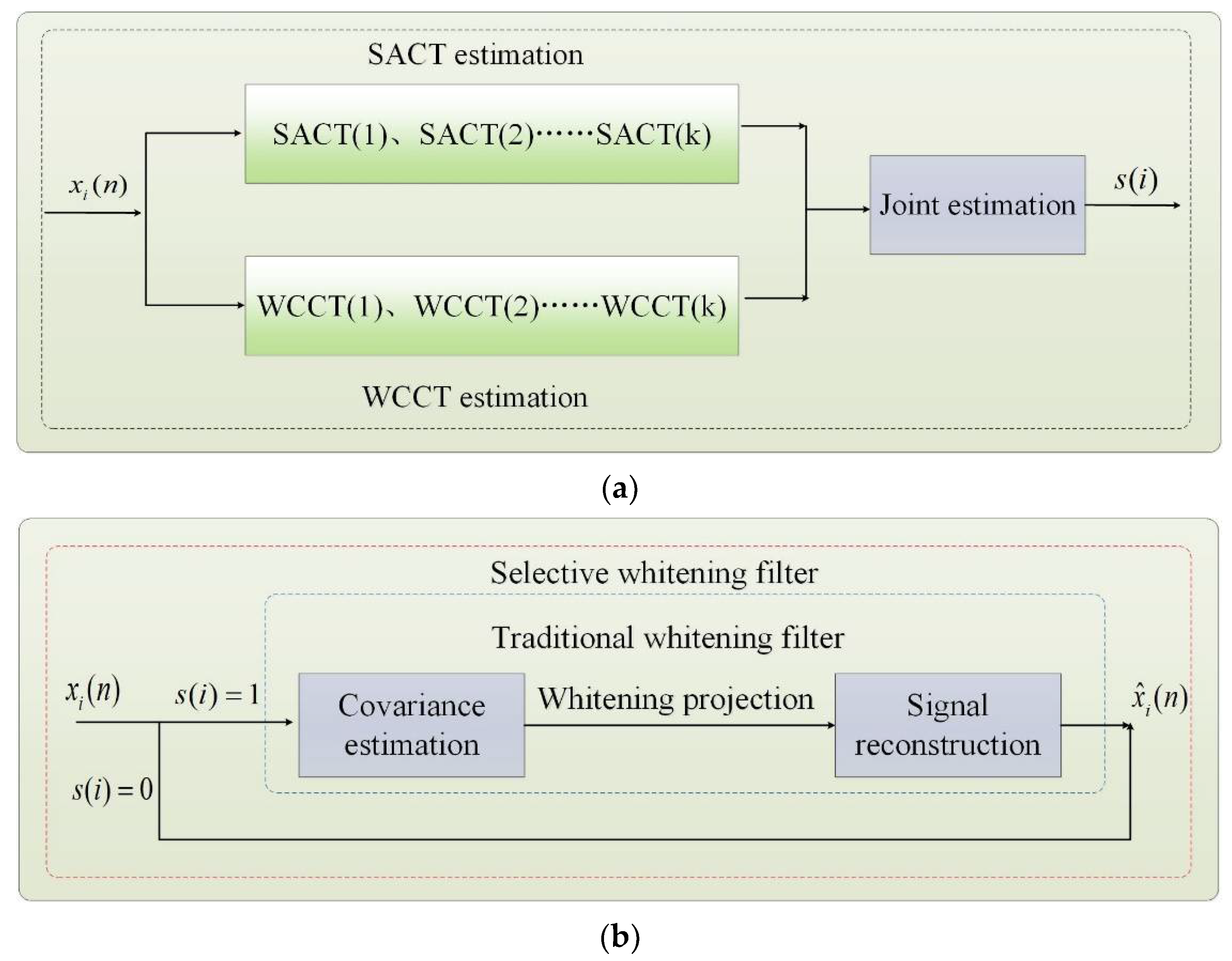
The sea clutter suppression stage is presented to effectively suppress the sea clutter, as shown in Figure 2. The suppression of sea clutter can be divided into two aspects: the suppression of sea clutter in different space range bins and the suppression of sea clutter in the target echo components.
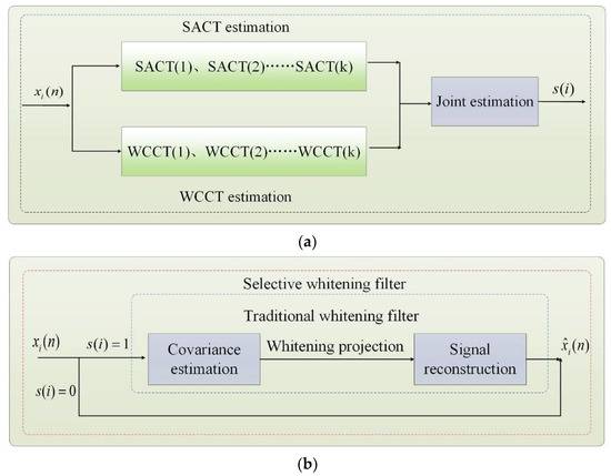
Figure 2.
Flow chart of the proposed sea clutter suppression stage. (a) Sea clutter suppression method based on correlation time estimation. (b) Selective whitening filter.
The sea clutter suppression method based on correlation time estimation is proposed to achieve the suppression of sea clutter in different space range bins. Traditional correlation estimation methods consider a single dimension and are easily disturbed by sea clutter. As shown in Figure 2a, both the SACT and WCCT of are considered in the proposed sea clutter suppression method, where denotes the echoes of a certain range bin. Besides, to enhance the estimation accuracy, the observation time is divided into several intervals, and multiple estimation results constitute the final estimation result, which makes the sea clutter suppression method more refined.
After the suppression of sea clutter in different space range bins, the whitening filter is adopted to suppress the sea clutter in the echo components. However, the traditional whitening filter is usually blind and requires a lot of calculation, in which all the range bins are whitened. To solve this problem, a selective whitening filter is illustrated in Figure 2b and is performed adaptively according to , where denotes the correlation estimation results.
In the next subsections, detailed information on the proposed sea clutter suppression stage is discussed.
2.1.1. Correlation Time of Sea Clutter in Time and Space Domains
The sea clutter is composed of the speckle component, the fast-changing capillary waves, and the modulation component, slow-changing gravity waves [25]. Within the period of energy accumulation, sea clutter shows a weak correlation, which is mainly determined by the speckle component. The target echoes have a stronger correlation than sea clutter because the target echoes are smoother. The time correlation coefficient of the time series is denoted as:
where represents the echoes of range bin. The signal is usually regarded as highly auto-correlated [26] when the correlation coefficient is between 0.5 and 1. In order to quantify the correlation coefficient, is defined as:
where is the time when the correlation coefficient drops from 1 to 0.5. The SACT of IPIX-#1 and IPIX-#11 are shown in Figure 3. The results marked by the red line are the corresponding results of the target bin. The results confirm that the target echoes and sea clutter differ in SACT, and the target echoes have stronger auto-correlation than sea clutter.

Figure 3.
Diagram of the SACT. (a) SACT of IPIX-#1. (b) SACT of IPIX-#11.
Simultaneously, the sea clutter at adjacent bins shows a certain correlation [25], while it is not correlated with the target echoes in the space domain. The space correlation coefficient of the time series of the range bin can be defined as:
where denotes the time sequence of the adjacent bin and denotes the number of the adjacent bin. Similarly, the is also defined as:
where is the time when the cross-correlation coefficient drops from 1 to 0.5. The WCCT of IPIX-#1 and IPIX-#11 are shown in Figure 4. The results confirm that the target echoes and sea clutter differ in WCCT and the target echoes have weaker cross-correlation compared to the sea clutter.
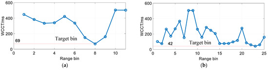
Figure 4.
Diagram of the WCCT. (a) WCCT of IPIX-#1. (b) WCCT of IPIX-#11.
To fully explain their differences in correlation time, statistical experiments are carried out on IPIX-1993 and IPIX-1998 data, and the observation time interval is 0.512 s. The experimental results are shown in Figure 5 and Figure 6.
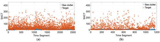
Figure 5.
Statistical results of the SACT. (a) SACT of IPIX-1993. (b) SACT of IPIX-1998.

Figure 6.
Statistical results of the WCCT. (a) WCCT of IPIX-1993. (b) WCCT of IPIX-1998.
In Figure 5, the SACT of the target is much higher than that of the sea clutter, and its statistical results almost drown the results of sea clutter. While in Figure 6, the WCCT of the target is smaller than that of the sea clutter, and the overlapping degree between the sea clutter and the target is higher than SACT, which is caused by the complex characteristics of the sea clutter. There is a certain correlation between the sea clutter of adjacent bins with a similar motion state. Still, if there are large fluctuations, the cross-correlation in space may decrease significantly.
When the observation time is 0.512 s, the SACT of sea clutter is only tens of milliseconds, while the SACT of target echoes can be up to hundreds of milliseconds. The WCCT of the target usually does not exceed 200 milliseconds, while the WCCT of sea clutter is mainly distributed between 200 and 500 milliseconds.
2.1.2. Sea Clutter Suppression Method Based on Correlation Time Estimation
The two related correlation time concepts proposed in Section 2.1.1 describe their correlation from the time dimension or the space dimension, respectively. They intuitively describe the correlation characteristics of sea clutter. However, there are many jump values in both statistical experiments. It is difficult to accurately describe the complex features of sea clutter in the time dimension or the space dimension.
In this work, a sea clutter suppression method based on correlation time estimation is then proposed, which can detect complex features in both the time and space dimensions. The correlation time of sea clutter is estimated in both time and space domains and is defined as:
where denotes the estimation results of and denotes the estimation results of . and are the corresponding threshold, which can be set according to specific experiments. To ensure the accuracy of the sea clutter correlation estimation, the echoes can be considered approximately stationary in a relatively short period of time [18,19]. The long observation time is divided into several intervals , and the judgment of each range bin is jointly determined by multiple intervals. It is defined as:
where denotes the sliding window within the observation time . Then, the two perception results, and , are jointly processed, and the operational relationship is shown in Equation (11):
where denotes the final estimation results as follows:
- (1)
- Suppose the estimation result of a particular range bin satisfies . In that case, it is regarded that the auto-correlation between the echoes of this range bin is strong, and the cross-correlation between the echoes in the adjacent range bin is weak. It is considered an interested bin.
- (2)
- Suppose the estimation result of a certain range bin satisfies . In that case, it is regarded that the auto-correlation between the echoes of this range bin is weak, or the cross-correlation between the echoes in the adjacent range bin is strong. It is considered a sea clutter bin.
The sea clutter in different space range bins can be suppressed by utilizing the estimation results. However, it is worth noting that the interested bins are completely preserved, and the sea clutter remains in the target echo component. To further achieve the suppression of the sea clutter in target echo components, the related method is discussed in Section 2.1.3.
2.1.3. Selective Whitening Filter Based on Correlation Estimation
A whitening filter is usually used for data pre-processing. The aim is to make the pulses of the same range bin not correlated with each other, and it is conducive to the extraction of subsequent feature components [27]. The principle of the whitening filter is to find a linear transformation so that the original data vector can become a whitening vector after being projected into a new subspace. It is defined as:
where is the time sequence of a certain range bin, is the whitening matrix, and is the whitening vector after processing. As for the whitening matrix , it can be obtained via principal component analysis. A transformation based on the calculation of the sample vector is defined as:
where is the covariance matrix and is the eigenvalue matrix of .
To avoid the influence of sea clutter power variation on covariance matrix estimation, the normalized sample covariance matrix estimation method (NSCM) is employed for calculation. The covariance matrix estimation is shown in Equation (14):
where denotes the number of pulses in a range bin, is the echo of the range bin, represents the conjugate transpose operation, and is the number of reference range bins. To improve the whitening effect, many proposed methods focus on the estimation of the covariance matrix [28,29,30]. However, such methods are generally blind and cannot effectively overcome the interference of sea clutter. In this work, a selective whitening filter is proposed, which is based on the estimation result in Section 2.1.2. It is performed on the “interested bins”, and the covariance matrix is calculated within the given range. The principle of the selective whitening filter is shown in Equation (15):
where represents the reconstructed data and denotes the whitening process. In this way, the signal is reconstructed, and the sea clutter is suppressed more effectively.
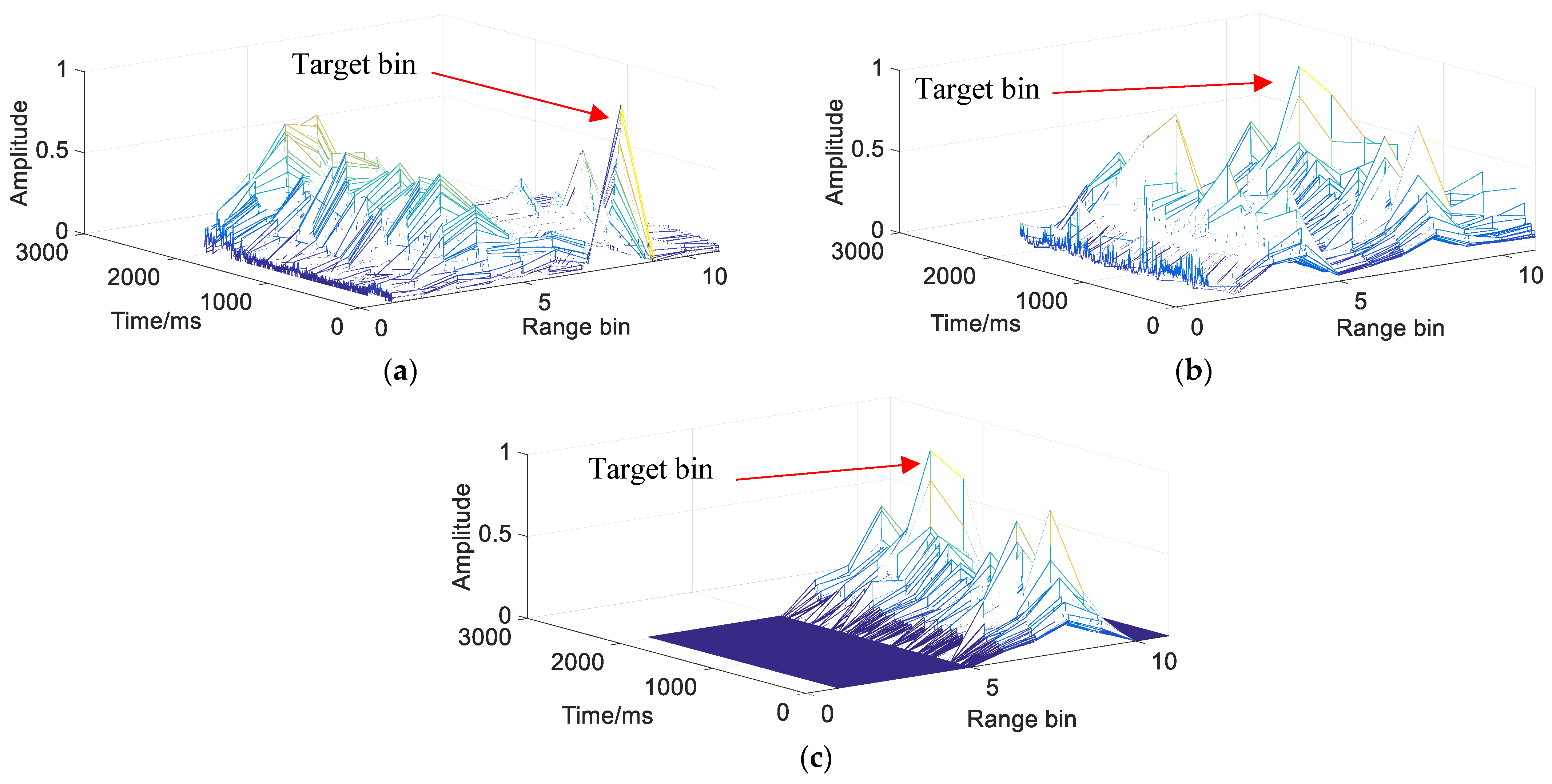
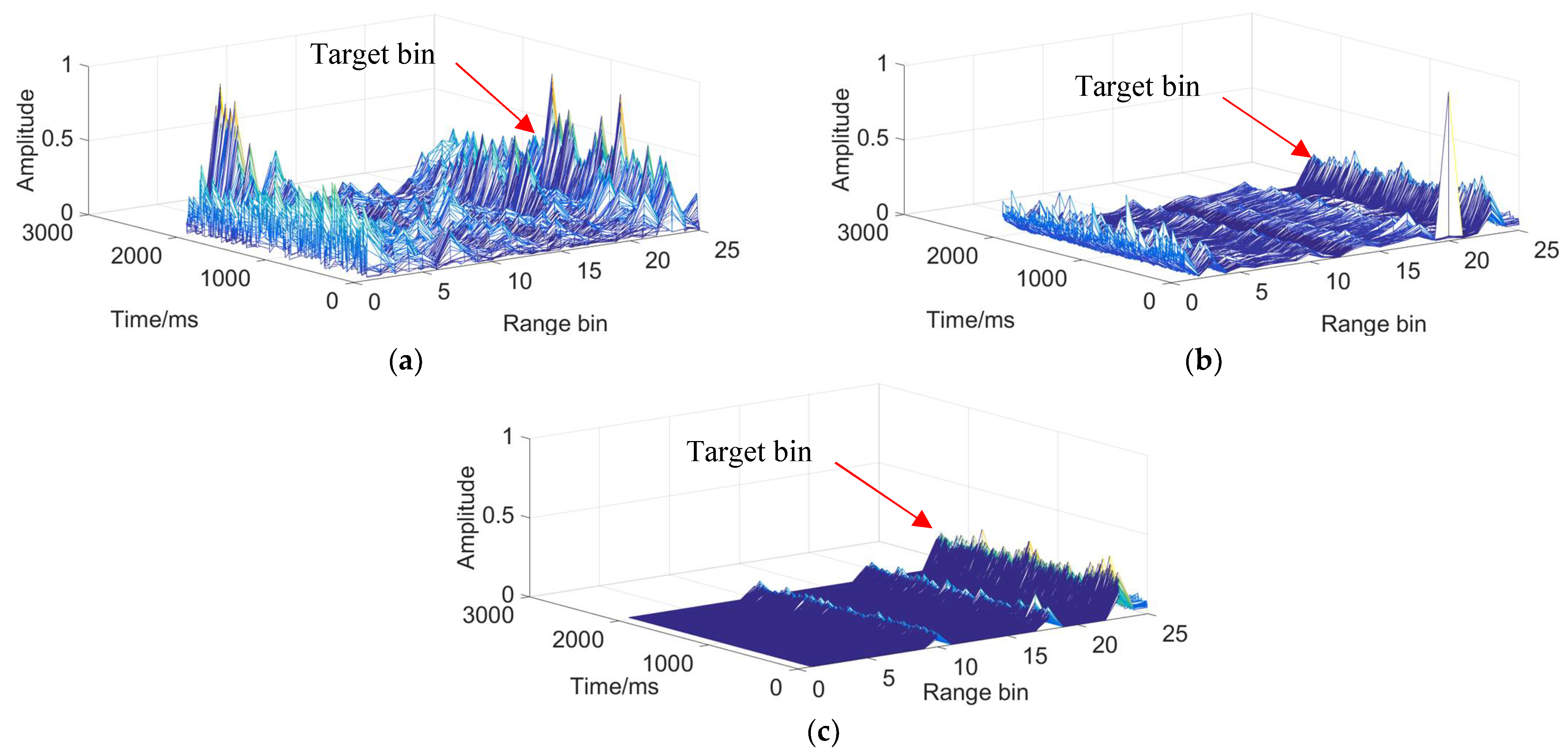
After using a traditional whitening filter, the sea clutter remains an obstacle to target observations in Figure 7b and Figure 8b, and the SNR in Figure 7b even decreases to 4.08 dB. As for the selective whitening filter, the SNR increase of the raw data is 6.6 dB and 10.34 dB in Figure 7c and Figure 8c, respectively. Not only is the sea clutter suppressed more greatly, but the observation of the target bin is also more intuitive in Figure 7c and Figure 8c. Besides, with this selective whitening filter, a large number of complex calculations around unnecessary sea clutter range bins are also avoided.

Figure 7.
Comparison results of whitening filter on IPIX-#1. (a) Raw data (5.70 dB). (b) Traditional whitening (4.08 dB). (c) Selective whitening (12.32 dB).

Figure 8.
Comparison results of whitening filter on IPIX-#11. (a) Raw data (6.70 dB). (b) Traditional whitening (10.24 dB). (c) Selective whitening(17.04dB).
2.2. Target Decision Stage
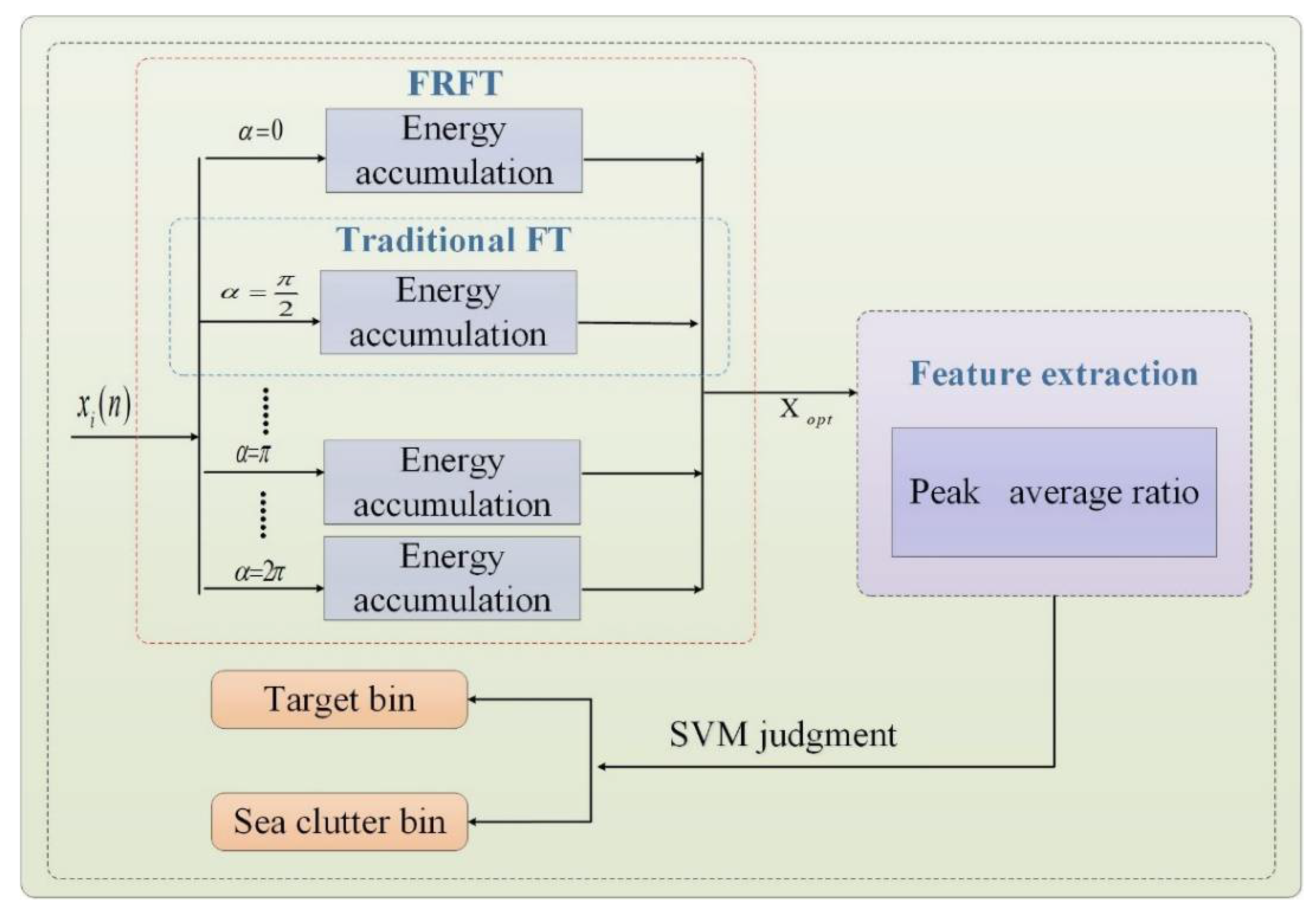
After the sea clutter suppression stage, the interference of sea clutter is reduced, and the SNR is also improved. Under this condition, a decision method based on long-time coherent integration is proposed. The FRFT is adopted to extract more advanced features, the peak average ratio (PAR), and a judgment model is built by SVM tools. The traditional extraction method of frequency PAR (F-PAR) [31] is based on the Fourier transform (FT), which is the only case when in Figure 9. As is illustrated in Figure 9, utilizing the FRFT will make the feature extraction more effective.
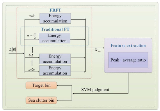
Figure 9.
Flow chart of the proposed decision methods.
The FRFT is the adaptation of the Fourier transform with fractional angles of 90 degrees [6,7,8,9]. Therefore, it has a better energy aggregation than the traditional Fourier transform. It is defined as:
where is the time sequence, is the rotation angle, and is the transform order, , . By searching for the peak point in the parameter plane, the optimal order of the transformation is determined. The is defined as:
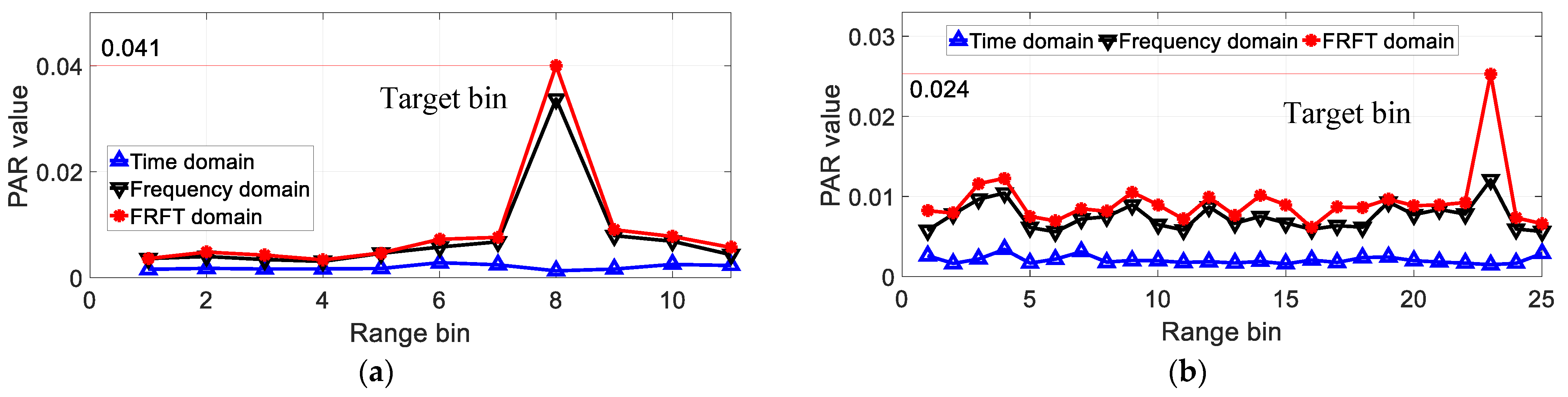
where is the transformation in the optimal order and is the length of time sequence . To demonstrate the reliability of the proposed FRFT detector, the raw data are directly used for tests and the comparisons between peak average ratio in the time domain (), , and are shown in Figure 10. The can attain a better energy aggregation for the LSS-target, and the peak characteristics of the target are more highlighted with the proposed .

Figure 10.
Comparison results of peak average ratio. (a) IPIX-#1. (b) IPIX-#11.
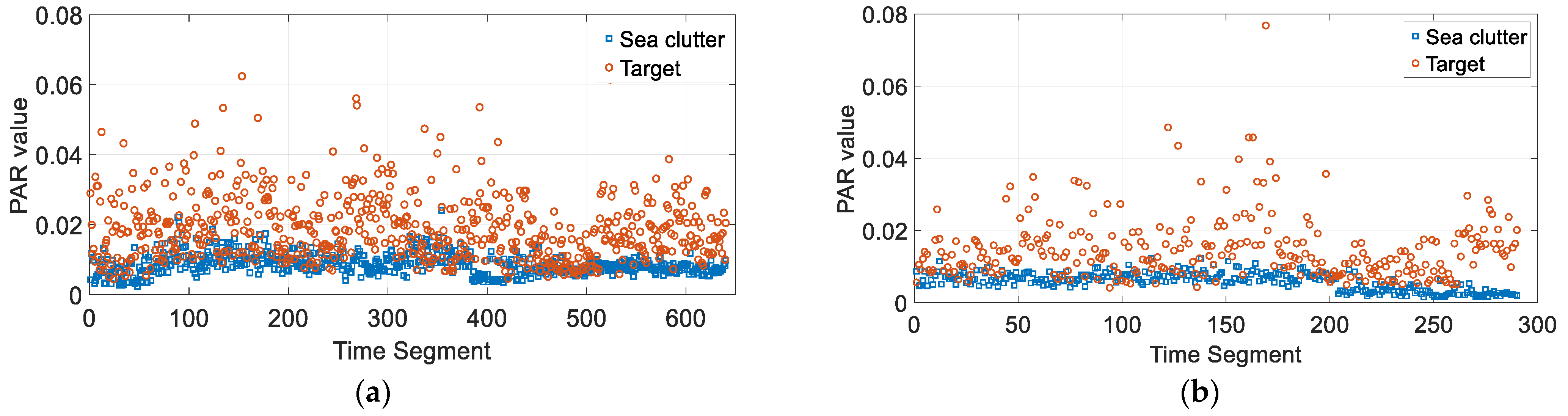
Furthermore, statistical experiments are also carried out, but the observation time is much longer and is 2.048 s. The experimental results are shown in Figure 11. Although there is some coupling in the statistical results, the overall distinction is clear. Experimentally, the value of the target is between 1% and 7%, while sea clutter is usually less than 1%.
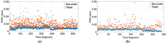
Figure 11.
Statistical results of the FRFT-PAR. (a) FRFT-PAR of IPIX-1993. (b) FRFT-PAR of IPIX-1998.
3. Results
3.1. Dataset Description
The detection performance of the proposed method is validated by the IPIX radar data. The IPIX database, a widely used database for sea surface small target detection, is collected by McMaster University in Canada. The test target in 1993 [18] is an anchored spherical block of Styrofoam, which is wrapped with wire mesh, and its diameter is about 1 m. Each dataset consists of complex echoes of 14 continuous range bins, and the length of the echoes in each bin is . Meanwhile, in 1998 [24], the test targets are floating boats. Each dataset consists of complex echoes of 28 continuous range bins, and the length of the echoes in each bin is . All the data have four polarization modes, namely, HH (horizontal transmit, horizontal receive), HV (horizontal transmit, vertical receive), VH (vertical transmit, horizontal receive), and VV (vertical transmit, vertical receive) polarizations. Besides, the two datasets have the same sampling frequency of 1 KHz in the slow time domain.
All the data can be divided into three categories, the pure sea clutter, the primary target bin, and the secondary bins. The main components of secondary bins are sea clutter, and only a small part of the target echoes are included. Its existence will make the characteristic analysis of sea clutter very complicated. For convenience, we only chose the pure sea clutter and primary range bin for the experiment, and the secondary bins were removed.
In Table 1, the detailed information about the datasets is described, including their file names in the IPIX database, wind speed (WS), significant wave height (SWH), the angle between the line of radar sight and wind direction, and the adjusted position information of the primary bins.

Table 1.
Descriptions of the datasets of the IPIX radar database.
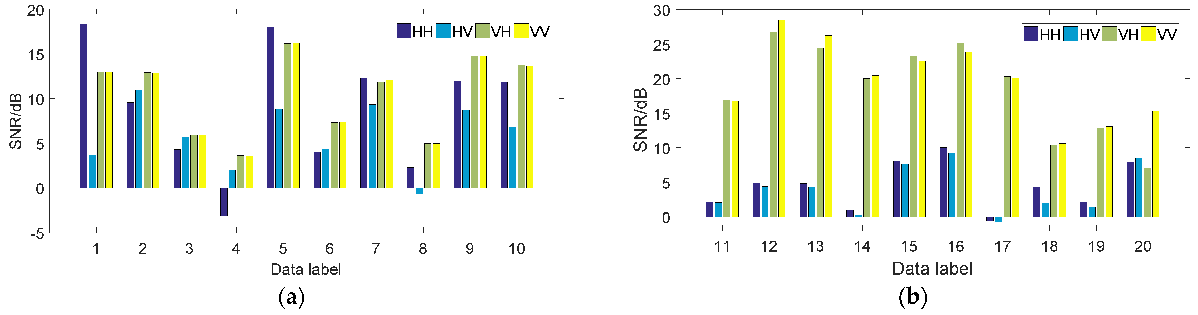
The SNR of the target bin is calculated as follows:
where denotes the length of time sequence and represents the average power of the sea clutter. The statistical results of ASNR are shown in Figure 12.
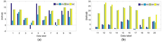
Figure 12.
Statistical results of data signal-to-noise ratio. (a) IPIX-1993. (b) IPIX-1998.
In addition, to illustrate the detection ability of different algorithms more specifically, the data in Table 1 are classified according to the average SNR. The classification results are shown in Table 2, and all the data are classified into 15 categories. In a word, they are evenly distributed, such as the low SNR interval [−1, 2.02], medium SNR interval [10.3, 10.8], and high SNR interval [16.5, 17].
Table 2.
Classification table of the average signal-to-noise ratio of IPIX radar data.
3.2. Comparison with the Existing Algorithms
To evaluate the robustness and effectiveness of the proposed method, several widely used methods based on sea clutter correlation analysis are taken for performance comparison. These methods include CF (the SACT in Section 2.1.1), CSM [22,23], and CANMF [18,19]. CF is the description of the auto-correlation of sea clutter, which uses the auto-correlation time to distinguish the sea clutter. CSM turns to the space domain and uses the signal synthesis method to decompose the space-time-frequency representation, which extracts the detection statistics from the decomposed components. CANMF is also conducted on the space domain and uses the reference bins to estimate the covariance matrix, which extracts the detection statistics from multiple frequency components.
The time sequence of length is grouped into equal observation time , and the detection results are obtained from different groups. Besides, the comparison experiments are also conducted under four polarizations. The observation time is selected as 2.048 s, and the false alarm rate is 0.001.
3.2.1. Detection Results on IPIX-1993 Dataset
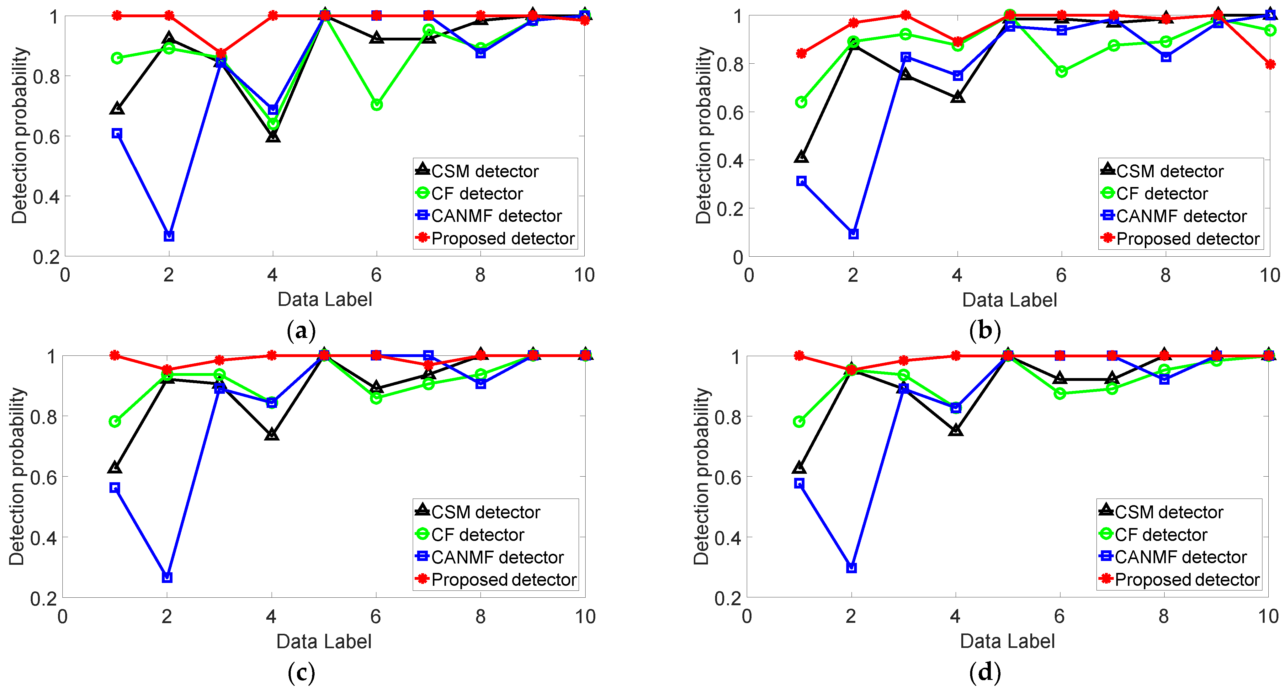
The detection results of different methods for the IPIX-1993 dataset are illustrated in Figure 13. It can be seen that the proposed method achieves the finest detection performance in four polarization modes. Because most sea clutter is suppressed in the suppression stage, and a pretty base is provided for the decision stage.
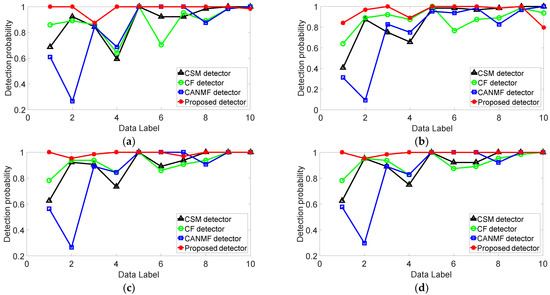
Figure 13.
Target detection results of IPIX-1993 dataset. (a) HH. (b) HV. (c) VH. (d) VV.
Compared with other methods, the detection performance of CF is maintained at a high level, but the overall curve fluctuates greatly because this single auto-correlation representation cannot respond to spatial changes. As for the CSM and CANMF, they show pretty detection performances at data. Although the spatial correlation is considered, their detection performances degrade sharply at data. Because their detection performances rely on the estimation of reference bins. If there are not enough ideal reference bins available, the sea clutter would remain as false alarms.
In addition, the test target in 1993 was an anchored spherical block of Styrofoam. Although it is wrapped with wire mesh, it is easy to rise and fall with the waves, which complicates its characteristics. This also explains why the detection curves of most methods show great fluctuations in Figure 13.
3.2.2. Detection Results on IPIX-1998 Dataset
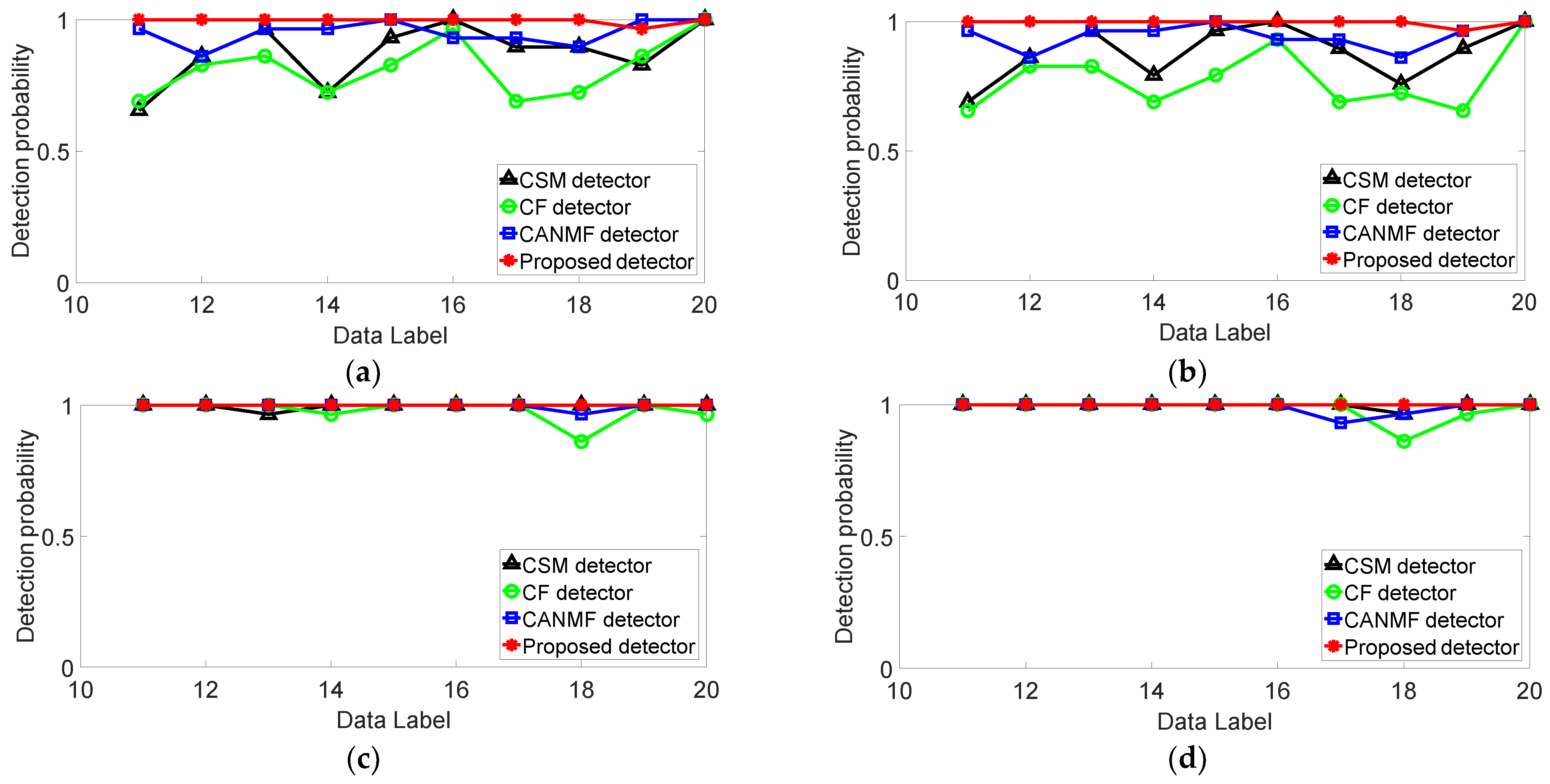
The detection results of different methods for the IPIX-1998 dataset are illustrated in Figure 14. It can be seen that the proposed method also achieves the finest detection performance in four polarization modes, and the detection probabilities of CSM and CANMF are slightly lower.
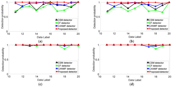
Figure 14.
Target detection results on IPIX-1998 dataset. (a) HH. (b) HV. (c) VH. (d) VV.
Compared with other methods, CSM and CANMF rely on the estimation of reference bins. For the IPIX-1998 dataset, the number of total range bins is twice the number of IPIX-1993. Therefore, more reference bins are available, and their detection performances are improved. For the detection performance of CF, Figure 14 shows a similar trend to Figure 13. Its detection performance still maintains a high level, but the overall curve fluctuates greatly in Figure 14 because there are more sea clutter range bins, and it cannot respond to spatial changes.
In addition, the test targets in 1998 were small boats with a more stable motion state and higher SNR in the echoes. This also explains why the detection curves of most methods show pretty detection performance in Figure 14.
3.3. Comprehensive Experimental Results
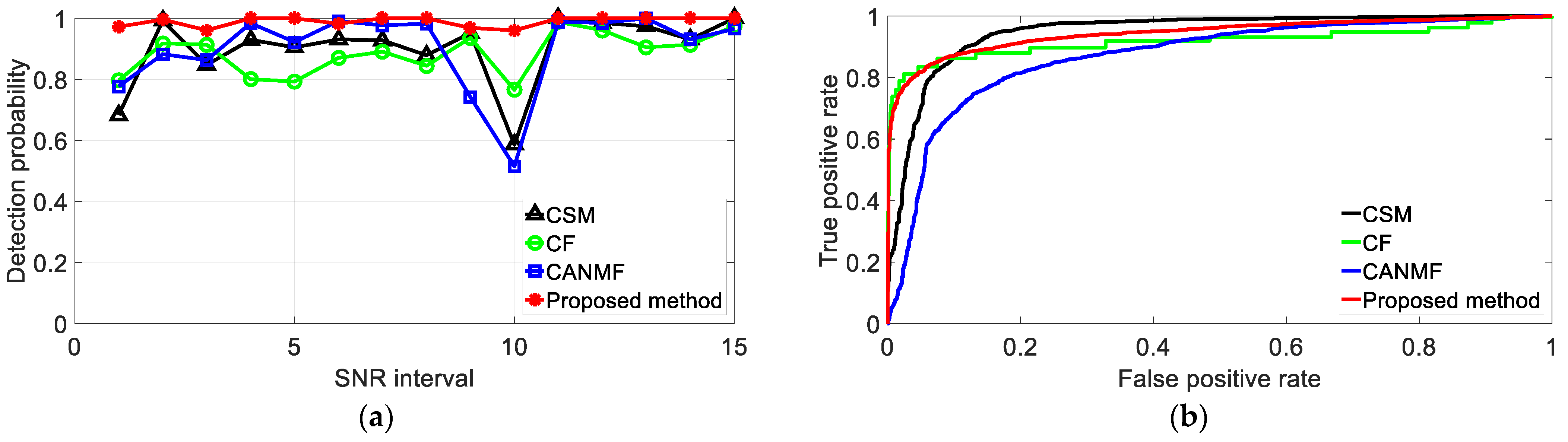
To make a more comprehensive analysis of the proposed algorithm, the average detection probabilities of the detectors on the 20 datasets are illustrated in Table 3. Figure 15a describes the detection rates of different algorithms changing with SNR. In the meantime, 3721 target samples and 3271 sea clutter samples were randomly extracted from the 20 datasets and Figure 15b describes the receiver operating curves (ROC) of different algorithms.
Table 3.
Average detection probabilities of the detectors on the 20 datasets at four polarizations.
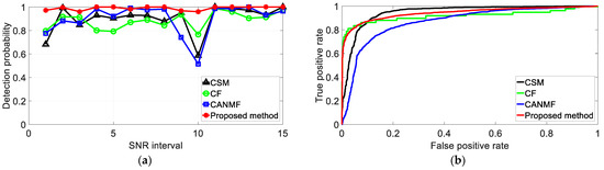
Figure 15.
Target detection probability (observation time 2.048 s). (a) Detection rates of different algorithms. (b) ROC curves of different algorithms.
The detection performances of most algorithms achieved about 2% to 10% improvement when the observation time doubled, as in Table 3. The sea clutter interferes with the target echoes, and more pulses are required to ensure high accuracy of target detection. However, the detection rates of most methods show large fluctuations in the whole SNR range in Figure 15a, especially at the interval. In such cases, extending observation time is not necessarily an optimal choice in improving the detection performance because it will also bring a heavy computational burden.
As for the proposed detector, its detection performance is not sensitive to observation time in Figure 15a and shows a more stable detection performance than other methods in Figure 15b. The average detection rate reaches 94% when the observation time is 0.512 s. The detection rate of CSM, CF, and CANMF could reach 90% when the observation time is 1.024 s or more.
4. Discussion
To further evaluate the effectiveness of the proposed sea clutter suppression stage, some experiments are carried out to analyze the effects of the sea clutter suppression stage.
4.1. Validation of the Sea Clutter Suppression Method
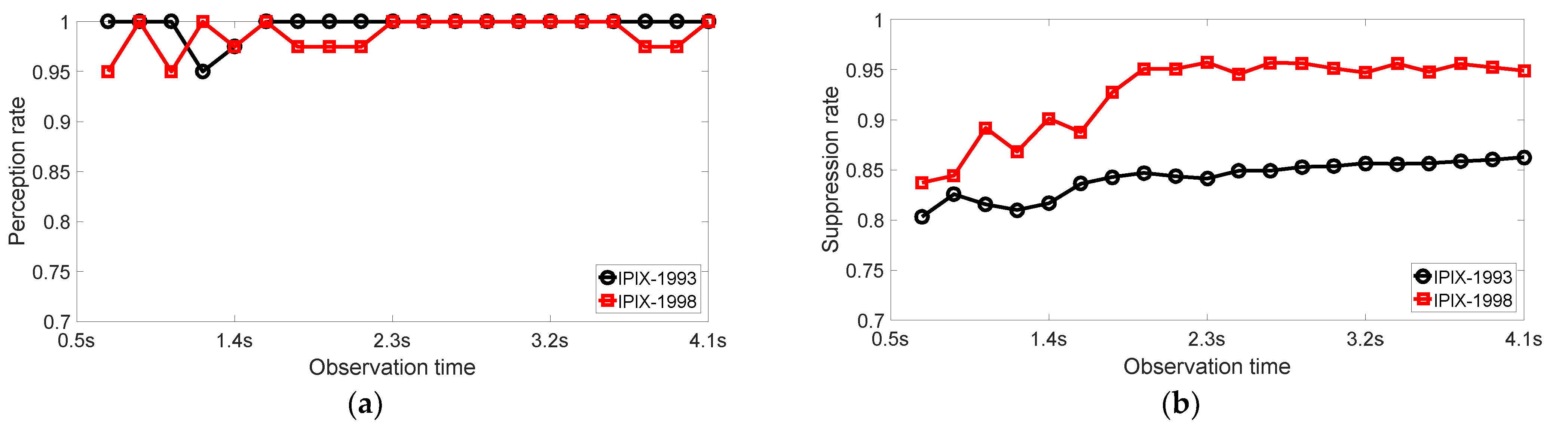
To illustrate the effectiveness of the proposed sea clutter suppression method, two indicators are introduced to validate its effectiveness. They are defined as:
where denotes the perception rate of the interested target bin, denotes the suppression rate of sea clutter, denotes the number of observation times that the target is perceived in observations, is the number of total range bins, and denotes the number of the suppressed range bins. The perception rate should be as close to 100% as possible to ensure that the target range bin could be retained. A high suppression rate of sea clutter should also be maintained, which is the key to removing the effect of sea clutter in different space range bins.
After many statistical experiments, the threshold in SACT is set to 50 milliseconds and the threshold in WCCT is set to 150 milliseconds. The perception rates and the suppression rates on the IPIX-1993 dataset and IPIX-1998 dataset are shown in Figure 16. The perception accuracy retains around 100% in Figure 16a, and 80% to 90% of range bins are suppressed in Figure 16b. The results show that the proposed estimation method can maintain a high sea clutter suppression rate while maintaining the perception rate.
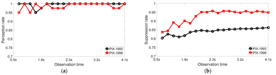
Figure 16.
Quantitative indicators of the proposed correlation estimation method. (a) perception rate. (b) suppression rate.
4.2. Validation of the Sea Clutter Suppression Stage
In this section, an ablation experiment was constructed to analyze the effects of the sea clutter suppression stage. The proposed detection method was compared to the long-time coherent integration strategy similar to FRFT-PAR. The RFT [11] and the fractal dimension (FD) in the FRFT domain (FRFT-FD) [15] were also added to confirm the effectiveness of the proposed sea clutter suppression stage. In this experiment, other settings were the same except for the sea clutter suppression stage.
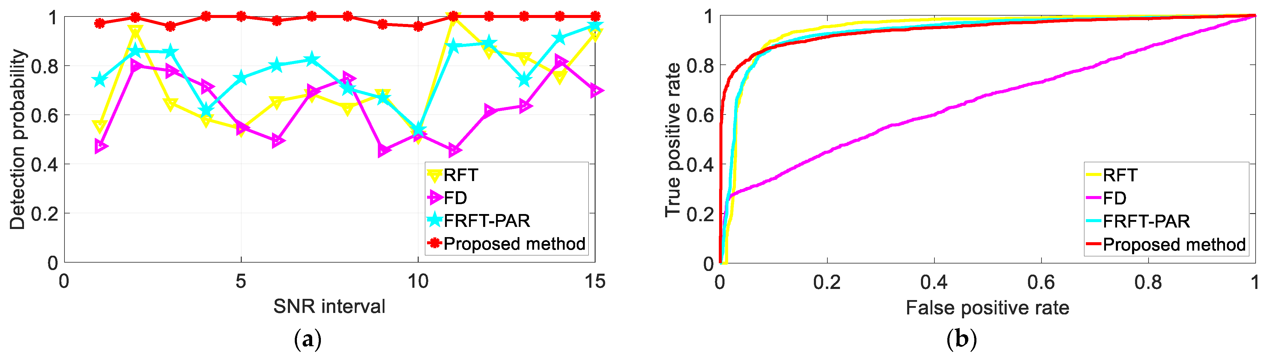
Figure 17a describes the changes in detection rate with SNR for different methods. Meanwhile, 3721 target samples and 3271 sea clutter samples were randomly extracted from the 20 datasets and Figure 17b describes the ROC curves of different algorithms. Table 4 gives their average detection performances at four polarization modes for different observation times.

Figure 17.
Target detection probability (observation time 2.048 s). (a) Detection rates of different algorithms. (b) ROC curves of different algorithms.
Table 4.
Average detection probabilities of the detectors on the 20 datasets at four polarizations.
The detection performances of the FRFT-PAR improved a lot with the help of the sea clutter suppression stage. When the observation time was 0.512 s, the detection rate of FRFT-PAR improved from 65.1% to 94.0% in HH polarization in Table 4. The maximum increase of the detection rate can reach 30%. Compared to other detection methods, the advantages of the proposed detection methods are even more obvious in Figure 17a,b. It holds a stable detection performance along the whole process in Figure 17a, while the detection curves of other algorithms show large fluctuations.
Besides, owing to the fact that the sea clutter is effectively suppressed by the sea clutter suppression stage, the computation cost of the proposed FRFT detector is moderate because the long-time coherent integration is completed in the few interested range bins. When the rotation angle obeys , the search step is 0.001, and the number of range bins is 100. The iteration times for one range bin are and the total iteration times are . With the sea clutter suppression, the iteration times can be reduced to , and about iteration times are reduced.
4.3. Comparison of the Computational Complexity
To evaluate the proposed method more intuitively, the computational complexity of different algorithms mentioned in this paper is illustrated in Table 5.
Table 5.
Computational complexity.
In Table 5, , , , , , and represent the number of range bins, the number of echoes, the group of the echoes, the number of the reference range bin, the number of iterations in FRFT, and the perception rate in Section 4.1, respectively. The procedures of the above algorithms mainly include the calculations of short-time Fourier transform (STFT), singular value decomposition (SVD), covariance matrix estimation, and FRFT. For the two-dimensional radar data, the calculations of STFT and FRFT can be solved by fast Fourier transform (FFT), and the computational complexity of FFT is . The computational complexity of SVD is , and the computational complexity of covariance matrix estimation is represented as .
As for the proposed detection method, the computation of the correlation estimation includes the calculation of SACT and WCCT, and its computational complexity is , which can be several times that of CF and RFT. Compared with CSM, CANMF, FD, and FRFT-PAR, the calculation of the selective whitening filter and target decision stage is much lower because it improves the selectivity of the calculation by correlation estimation, and the total computational complexity is . In this way, a lot of computations are saved.
In a word, the computational complexity of the method proposed in this paper was increased compared with other methods, but it is generally controlled within a certain range.
5. Conclusions
A low observable radar target detection method based on sea clutter correlation estimation is proposed in this paper, which consists of the sea clutter suppression stage and target detection stage. In the sea clutter suppression stage, the correlation time differences in the time domain and the space domain are adopted to estimate the correlation of sea clutter. According to the estimation results, the sea clutter in different range bins is suppressed. After that, a selective whitening filter is presented, which is performed more adaptively according to the estimation results and can facilitate the suppression of the sea clutter in the echo components. In the decision stage, the peak average ratio in the fractional Fourier domain (FRFT-PAR) is presented, which is adopted to make better use of the energy accumulation characteristics and further suppress the interference of sea clutter. Experiments on the IPIX datasets with various observation times and polarization modes are included. The results indicate that the proposed detection method can effectively suppress the sea clutter and achieve better target detection performance than baseline algorithms. Besides, the computational complexity of the proposed detection method is also controlled within a certain range.
However, the detection performance of the proposed detection method depends on the accuracy of correlation estimation. The thresholds of the proposed correlation estimation are derived from the statistical experiments, which are not adaptive and need to be adjusted in different scenarios. Furthermore, the proposed detection method is not tested with the secondary bin, whose existence will make the characteristic analysis of sea clutter more complicated. The way to maintain more steady detection performances will be our future works.
Author Contributions
Conceptualization, Z.L. (Zhengzhou Li); Methodology, Z.L. (Zefeng Luo); Software, Z.L. (Zefeng Luo); Validation, Z.L. (Zhengzhou Li), J.D. and C.Z.; Investigation, Z.L. (Zhengzhou Li); Resources, T.Q.; Data curation, T.Q.; Writing—Original Draft Preparation, Z.L. (Zefeng Luo); Writing—Review and Editing, Z.L. (Zefeng Luo) and Z.L. (Zhengzhou Li); Visualization, J.D.; Supervision, Z.L. (Zhengzhou Li); Project Administration, T.Q. All authors have read and agreed to the published version of the manuscript.
Funding
This work was partially supported by the National Natural Science Foundation of China under Grant No. 61675036, 13th Five-year Plan Equipment Pre-Research Fund under Grant No. 6140415020312, and Chinese Academy of Sciences Key Laboratory of Beam Control Fund under Grant No. 2017LBC006.
Conflicts of Interest
The authors declare no conflict of interest. The funders had no role in the design of the study; the collection, analyses, or interpretation of data; the writing of the manuscript; or the decision to publish the results.
References
- Ma, L.; Wu, J.; Zhang, J.; Wu, Z.; Jeon, G.; Tian, M.; Zhang, Y. Sea Clutter Amplitude Prediction Using a Long Short-Term Memory Neural Network. Remote Sens. 2020, 11, 2826. [Google Scholar] [CrossRef] [Green Version]
- Liu, X.; Xu, S.; Tang, S. CFAR Strategy Formulation and Evaluation Based on Fox’s H-function in Positive Alpha-Stable Sea Clutter. Remote Sens. 2020, 12, 1273. [Google Scholar] [CrossRef] [Green Version]
- Yang, Z.; Tang, J.; Zhou, H.; Xu, X.; Tian, Y.; Wen, B. Joint Ship Detection Based on Time-Frequency Domain and CFAR Methods with HF Radar. Remote Sens. 2021, 13, 1548. [Google Scholar] [CrossRef]
- Chen, X.; Guan, J.; Mu, X.; Wang, Z.; Liu, N.; Wang, G. Multi-Dimensional Automatic Detection of Scanning Radar Images of Marine Targets Based on Radar PPInet. Remote Sens. 2021, 13, 3856. [Google Scholar] [CrossRef]
- Yan, H.; Chen, C.; Jin, G.D.; Zhang, J.; Wang, X.; Zhu, D. Implementation of a Modified Faster R-CNN for Target Detection Technology of Coastal Defense Radar. Remote Sens. 2021, 13, 1703. [Google Scholar] [CrossRef]
- Fang, X.; Cao, Z.; Min, R.; Pi, Y. Radar Maneuvering Target Detection Based on Two Steps Scaling and Fractional Fourier Transform. Signal Process. 2019, 155, 1–13. [Google Scholar]
- Chen, X.; Guan, J.; Yu, X.; He, Y. Radar Micro-Doppler Signature Extraction and Detection Via Short-Time Sparse Time-Frequency Distribution. J. Electron. Inf. Technol. 2017, 39, 1017–1023. [Google Scholar]
- Chen, X.; Guan, J.; Bao, Z.; He, Y. Detection and Extraction of Target with Micromotion in Spiky Sea Clutter via Short-Time Fractional Fourier Transform. IEEE Trans. Geosci. Remote Sens. 2014, 52, 1002–1018. [Google Scholar] [CrossRef]
- Liu, S.; Shan, T.; Tao, R.; Zhang, Y.; Zhang, G.; Zhang, F.; Wang, Y. Sparse Discrete Fractional Fourier Transform and Its Applications. IEEE Trans. Signal Process. 2014, 62, 6582–6595. [Google Scholar] [CrossRef] [Green Version]
- Xu, J.; Yu, J.; Peng, Y.; Xia, X. Radon-Fourier Transform for Radar Target Detection, I: Generalized Doppler Filter Bank. IEEE Trans. Aerosp. Electron. Syst. 2011, 47, 1186–1202. [Google Scholar] [CrossRef]
- Xu, J.; Zhou, X.; Qian, L.; Xia, X.; Long, T. Hybrid Integration for Highly Maneuvering Radar Target Detection Based on Generalized Radon-Fourier Transform. IEEE Trans. Aerosp. Electron. Syst. 2016, 52, 2554–2561. [Google Scholar] [CrossRef]
- Chen, X.; Guan, J.; Liu, N.; He, Y. Maneuvering Target Detection via Radon-Fractional Fourier Transform-Based Long-Time Coherent Integration. IEEE Trans. Signal Process. 2014, 62, 939–953. [Google Scholar] [CrossRef]
- Luo, F.; Zhang, D.; Zhang, B. The Fractal Properties of Sea Clutter and Their Applications in Maritime Target Detection. IEEE Geosci. Remote Sens. Lett. 2013, 10, 1295–1299. [Google Scholar] [CrossRef]
- Li, Y.; Yang, Y.; Zhu, X. Target Detection in Sea Clutter Based on Multifractal Characteristics after Empirical Mode Decomposition. IEEE Geosci. Remote Sens. Lett. 2017, 14, 1547–1551. [Google Scholar] [CrossRef]
- Chen, X.; Guan, J.; He, Y.; Zhang, J. Detection of low observable moving target in sea clutter via fractal characteristics in fractional Fourier transform domain. IET Radar 2013, 7, 635–651. [Google Scholar] [CrossRef]
- Kammoun, A.; Couillet, R.; Pascal, F.; Alouini, M. Optimal Design of the Adaptive Normalized Matched Filter Detector Using Regularized Tyler Estimators. IEEE Trans. Aerosp. Electron. Syst. 2015, 52, 755–769. [Google Scholar] [CrossRef] [Green Version]
- He, Y.; Jian, T.; Su, F.; Qu, C.; Ping, D. Adaptive Detection Application of Covariance Matrix Estimator for Correlated Non-Gaussian Clutter. IEEE Trans. Aerosp. Electron. Syst. 2010, 46, 2108–2117. [Google Scholar] [CrossRef]
- Shui, P.; Li, D.; Xu, S. Tri-Feature-Based Detection of Floating Small Targets in Sea Clutter. IEEE Trans. Aerosp. Electron. Syst. 2014, 50, 1416–1430. [Google Scholar] [CrossRef]
- Xu, S.; Shui, P.; Yan, X.; Cao, Y. Combined Adaptive Normalized Matched Filter Detection of Moving Target in Sea Clutter. Circuits Syst. Signal Process. 2017, 36, 2360–2383. [Google Scholar] [CrossRef]
- Stankovic, L.; Thayaparan, T.; Dakovic, M. Signal decomposition by using the S-method with application to the analysis of HF radar signals in sea-clutter. IEEE Trans. Signal Process. 2006, 54, 4332–4342. [Google Scholar] [CrossRef]
- Stankovic, L.; Mandic, D.; Dakovic, M.; Brajovic, M. Time-frequency decomposition of multivariate multicomponent signals. Signal Process. 2017, 142, 468–479. [Google Scholar] [CrossRef]
- Zuo, L.; Li, M.; Zhang, X.; Zhang, P.; Wu, Y. CFAR Detection of Range-Spread Targets Based on the Time-Frequency Decomposition Feature of Two Adjacent Returned Signals. IEEE Trans. Signal Process. 2013, 61, 6307–6319. [Google Scholar] [CrossRef]
- Lee, M.; Kim, J.; Ryu, B.; Kim, K.T. Robust Maritime Target Detector in Short Dwell Time. Remote Sens. 2021, 13, 1319. [Google Scholar] [CrossRef]
- Shi, S.; Shui, P. Sea-Surface Floating Small Target Detection by One-Class Classifier in Time-Frequency Feature Space. IEEE Trans. Geosci. Remote Sens. 2018, 56, 6395–6411. [Google Scholar] [CrossRef]
- Liu, H.; Song, J.; Xiong, W.; Cui, Y.; Lv, Y.; Liu, J. Analysis of Amplitude Statistical and Correlation Characteristics of High Grazing Angle Sea-Clutter. J. Eng.-Joe 2019, 2019, 6829–6833. [Google Scholar] [CrossRef]
- Xiong, G.; Xi, C.; Li, D.; Yu, W. Cross Correlation Singularity Power Spectrum Theory and Application in Radar Target Detection within Sea Clutters. IEEE Trans. Geosci. Remote Sens. 2019, 57, 3753–3766. [Google Scholar] [CrossRef]
- Choi, S.; Yang, H.; Song, J.; Jeon, H.; Chung, Y. Sea Clutter Covariance Matrix Estimation and Its Application to Whitening Filter. J. Electromagn. Eng. Sci. 2021, 21, 134–142. [Google Scholar] [CrossRef]
- De Miao, A.; Pallotta, L.; Li, J.; Stoica, P. Loading Factor Estimation Under Affine Constraints on the Covariance Eigenvalues With Application to Radar Target Detection. IEEE Trans. Aerosp. Electron. Syst. 2019, 55, 1269–1283. [Google Scholar] [CrossRef]
- Conte, E.; De Miao, A.; Li, J. Mitigation Techniques for Non-Gaussian Sea Clutter. IEEE J. Ocean. Eng. 2004, 29, 284–302. [Google Scholar] [CrossRef]
- Greco, M.; Stinco, P.; Gini, F.; Rangaswamy, M. Impact of Sea Clutter Nonstationarity on Disturbance Covariance Matrix Estimation and CFAR Detector Performance. IEEE Trans. Aerosp. Electron. Syst. 2010, 46, 1502–1513. [Google Scholar] [CrossRef]
- Li, Y.; Xie, P.; Tang, Z.; Jiang, T.; Qi, P. SVM-Based Sea-Surface Small Target Detection: A False-Alarm-Rate-Controllable Approach. IEEE Geosci. Remote Sens. Lett. 2019, 16, 1225–1229. [Google Scholar] [CrossRef] [Green Version]
Publisher’s Note: MDPI stays neutral with regard to jurisdictional claims in published maps and institutional affiliations. |
© 2022 by the authors. Licensee MDPI, Basel, Switzerland. This article is an open access article distributed under the terms and conditions of the Creative Commons Attribution (CC BY) license (https://creativecommons.org/licenses/by/4.0/).