Technical Note

First Earth-Imaging CubeSat with Harmonic Diffractive Lens

1
Image Processing Systems Institute of the RAS—Branch of the Federal Scientific Research Centre “Crystallography and Photonics” of the Russian Academy of Sciences, Molodogvardeyskaya 151, 443001 Samara, Russia
2
Samara National Research University, Moskovskoye Shosse 34, 443086 Samara, Russia
3
National Research University Higher School of Economics, 20 Myasnitskaya Ulitsa, 101000 Moscow, Russia
*
Author to whom correspondence should be addressed.
Remote Sens. 2022, 14(9), 2230; https://doi.org/10.3390/rs14092230
Submission received: 11 March 2022 / Revised: 25 April 2022 / Accepted: 1 May 2022 / Published: 6 May 2022
(This article belongs to the Special Issue Cubesats for Scientific and Civil-Use Studies of the Earth)

Abstract

:
Launched in March 2021, the 3U CubeSat nanosatellite was the first ever to use an ultra-lightweight harmonic diffractive lens for Earth remote sensing. We describe the CubeSat platform we used; our 10 mm diameter and 70 mm focal length lens synthesis, design, and manufacturing; a custom 3D-printed camera housing built from a zero-thermal-expansion metal alloy; and the on-Earth image post-processing with a convolutional neural network resulting in images comparable in quality to classical refractive optics used for remote sensing before.

1. Introduction

Nanosatellites opened new opportunities for remote sensing applications. Due to their small size and low cost, swarms of CubeSat nanosatellites can be put into orbit for continuous monitoring of the ionosphere, atmosphere, clouds, and the Earth’s surface [1,2,3]. However, due to the small volume of the CubeSat, strict miniaturization constraints are imposed on the payload dimensions, weight, and energy consumption. Since conventional refractive remote sensing lenses have a relatively large mass and dimensions, adding long-focal-length optics to nanosatellites has always been challenging due to their linear dimension limitations [4]. The use of diffractive lenses in the nanosatellite optical system has several advantages over refractive lenses, especially their lower mass and thickness, since the lens microrelief is synthesized within thin flat substrates. With a flat lens, the overall dimensions of the optical system can be reduced, and a longer focal length lens can fit into the satellite, yielding a better spatial resolution of the Earth’s surface for a given satellite size. This gives diffractive optics a clear advantage for nanosatellites.
A diffractive lens, however, forms an image with high chromatic aberrations, which can be reduced by creating a thicker lens microrelief, from about 500 nm to 10 μm, and by reducing the lens fabrication errors [5]. The resulting diffractive lenses are called harmonic lenses [6]. The imaging quality could be also improved by computer-aided processing using deconvolution [7,8] or neural-network-aided reconstruction [9,10,11,12,13].
The use of a flat diffractive lens in remote sensing and space exploration has been studied before. One of the first working prototypes with a 20-m diameter membrane diffractive lens as an imaging system was a DARPA project called “Membrane Optical Imager for Real-Time Exploitation” (MOIRE), which was initiated in 2012 [14] and passed the laboratory tests in 2014 [15]. However, there is no public information confirming the launch or success of a MOIRE space mission. A diffractive lens [7] is considered to be one of the imaging technologies for a “Breakthrough Starshot” interstellar picosatellite project [16]. More recent studies include a telescope based on a diffractive lens [17], an array of diffractive lenses [18], and a membrane diffractive lens [19,20]. Despite this progress, none of these telescopes has been sent to space. The TOLIMAN space telescope with a diffraction pupil lens was announced in 2018 [21].
In this work, we discuss design decisions, image reconstruction, and the results of the first in-orbit experimental study of images produced by a 3U CubeSat nanosatellite with an ultra-lightweight remote sensing camera based on our harmonic diffractive lens designed from the ground up in our lab. This lens is significantly lighter and thinner than a conventional refractive lens of a similar focal length and aperture, as we described in our previous work [10] in more detail.

2. A CubeSX-HSE Nanosatellite-Based Remote Sensing Platform

2.1. Nanosatellite Design

The CubeSX-HSE nanosatellite was created by the Moscow Institute of Electronics and Mathematics at the National Research University Higher School of Economics (HSE). Its design is based on the 3U CubeSat platform OrbiCraft-Pro [22]. With this modular platform, new satellites can be rapidly configured from pre-designed components, off-the-shelf electronics, and open-source software libraries.

2.1.1. Data Transmission System

The OrbiCraft-Pro ultrashort-wave transducer SXC-UHF-02 is implemented on a separate board connected to the satellite’s main electronic module board with a PC/104 connector [22]. The transducer operational frequency can be tuned within a 434–436 MHz range, with a 20 kHz passband. This enables a data transmission rate of 9600 baud in the Gaussian minimum-shift keying (GMSK) modulation mode, sufficient for exchanging telemetry, commands, and the payload data. The maximum output power of 1 W and the sensitivity of 119 dB are optimized for the data transmission from a low Earth orbit (LEO). The ultrashort-wave transducer operates in the temperature range of −40 to +85 °C and weighs ~40 g. The transducer is compatible with the OrbiCraft-Pro PC/104 interface, provides an additional universal asynchronous receiver-transmitter (UART), and enables the transmission of heartbeat packages and onboard time signals to the onboard CAN bus.
The onboard high-speed radio transmitter SXC-XTX-01 can send data to the Earth at a rate of 10 Mbit in the X-band (8175–8215 MHz) [22] and is also connected to the onboard bus CAN2.0B with a unified connector PC/104.

2.1.2. Hardware Configuration

CubeSX-HSE is a small satellite made up of three 10 × 10 × 10 cm cubic units on a single aluminum alloy frame. One unit contains a set of flywheels for the satellite spatial orientation, the second unit houses circuit boards for the satellite control, and the third unit is entirely dedicated to the payload, in our case a diffractive-lens-based remote sensing camera.
The OrbiCraft-Pro platform was designed for the manual assembly of its electronic and mechanical components into a CubeSat nanosatellite [23]. The Pro modification represents an assembled and manufacturer-approved platform version that has passed a complete set of qualification tests. It has a three-axis orientation and stabilization system and gallium arsenide photoelectric transducers, and it can be integrated with a custom payload. Included are printed circuit boards linked together with PC/104 connectors, where each board implements one or several satellite functions; the platform also includes cables, solar cells, and power supply elements [24].
The main unit contains three connected components: the main stack of electronic circuit boards, a mounting frame, and solar panels, as shown in Figure 1a.
The electronics are designed to be modular, and the position of modules in the satellite card cage can be varied. Various modules connected to the PC/104 bus can be installed into the vertical stack cage; these include an orientation and stabilization system controller, various payload boards, and other modules, as shown in Figure 1b. Each system is connected to the CAN2.0B-based internal satellite network operating at 1 Mbit/s. A high-level UniCAN 2.0 protocol runs on top of the CAN2.0B protocol stack to ensure reliable and convenient telemetry and command reception/transmission. The satellite cabling utilizes extensible PC/104 connections, including connections to the service board and side-face devices such as solar panels. The service board is connected to the satellite communication system and the battery charging interface, and it has a multiplexed two-wire interface to test and update the firmware without the need to remove electronic boards from the assembled satellite. The solar sensors are mounted on all sides of the satellite frame and protected by dedicated side-panel windows.
An easy-to-assemble, rugged satellite frame provides convenient access to the internals [24]. The satellite is separated from the launch container into its orbit with two spring pushers and duplicated circuit breakers with slots for connecting with the SXC-PSU-03 power unit. Mounted at the bottom of the satellite, the separation system has two spring-loaded switches located at the ends of a diagonal rail and may include two separating springs. During the transportation and storage, the switches are off and the battery is disconnected. When in orbit, the springs are activated, ejecting the satellite from a launch container P-POD to the outer space, closing the switches, and connecting the battery pack to the satellite power circuit.

2.2. Satellite Flight Characteristics

The CubeSX-HSE nanosatellite launched into a 570 km orbit on 22 March 2021, carried by a Soyuz-2.1a rocket with a Fregat upper stage. Figure 2 shows the 3.5 kg satellite after the assembly. The camera unit with an aperture opening can be seen on the right side of the satellite assembly in the second picture below.
The satellite three-axis orientation and stabilization system has solar sensors, a four-motor flywheel module, and a microcontroller located on the motherboard.

2.3. Onboard Computing Module

An onboard computing module (BCM) SXC-MB-04 controls the satellite and hosts the following components [22]:
-
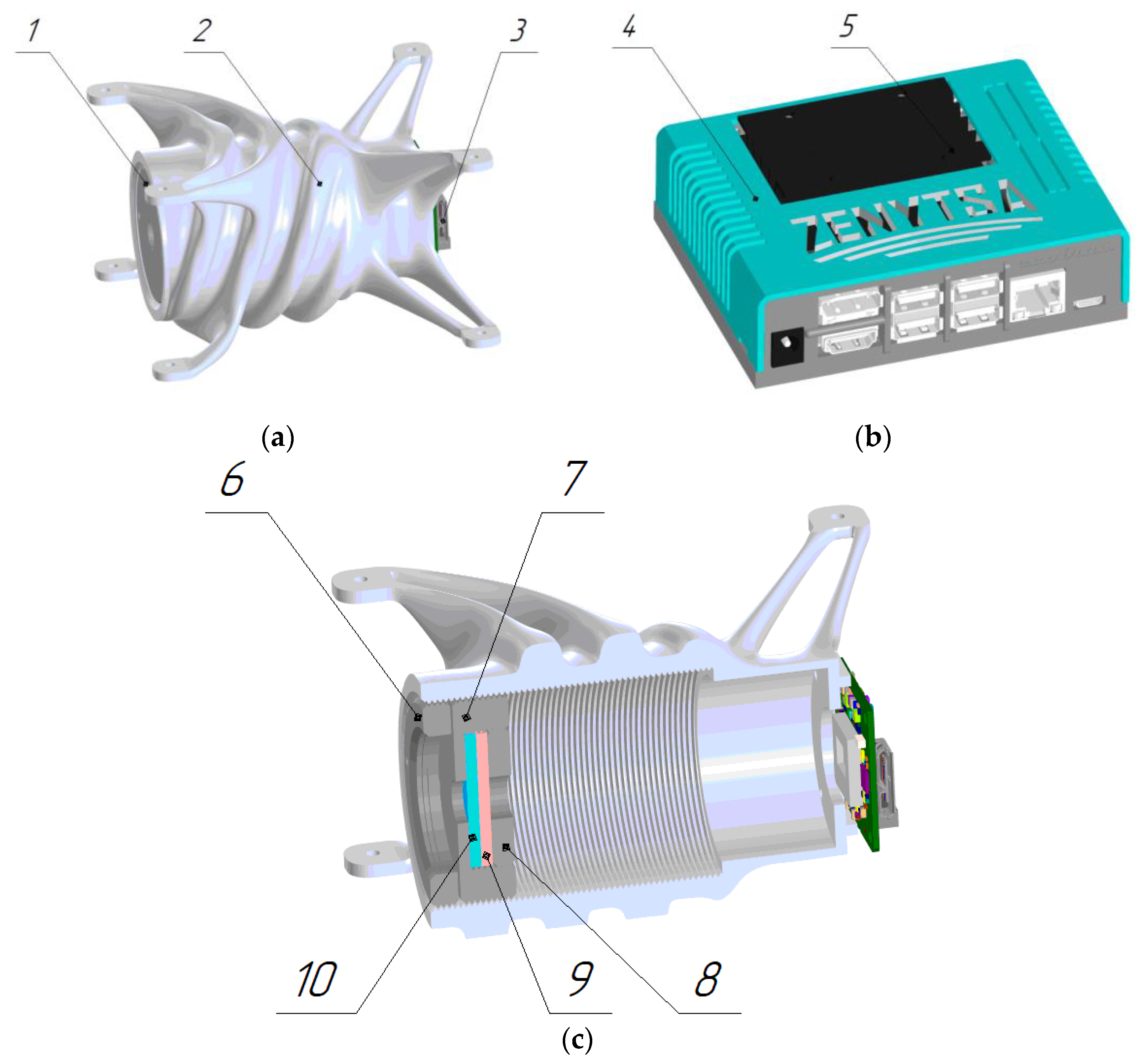
A slot for connecting a Raspberry CM3 processing module with a power supply system;
-
An autonomous controller of the orientation and stabilization system;
-
An energy-saving sensor microcontroller;
-
A gyroscope and magnetometer;
-
A unit for electromagnetic coil control;
-
A temperature sensor;
-
A real-time clock with a battery backup;
-
A power supply system;
-
A centralized programming and software testing system.
All onboard devices can be accessed through an onboard bus CAN2.0B directly, while the Raspberry module is connected with an SPI-CAN converter. The motherboard can support Raspberry Pi CM3 and CM3+ modules. Once the satellite is assembled, all microcontrollers become available for firmware installation and testing. A detachable Wi-Fi module and video interfaces are installed directly onto the Raspberry Pi 3 module. With all electronics assembled, the board weighs 55 g and operates in the −40 to +85 °C temperature range.
To operate the three-axis orientation and stabilization system, six solar sensors are used [22]. A built-in orientation and stabilization system microcontroller works autonomously, using a CAN interface for the command and telemetry reception and transmission. The energy-saving microcontroller is connected to sensors with a CAN interface and directs the space mission by controlling the onboard systems while optimizing the energy consumption of the main computing module. The stabilization using the B-dot algorithm [24] can be autonomously activated using the built-in induction coil driver.
The energy-efficient performance is ensured by the proper BCM hierarchy, where each operation mode is controlled by a dedicated microcontroller:
-
An energy-efficient microcontroller for data acquisition;
-
An orientation and stabilization system controller activated when needed;
-
Raspberry Pi 3 for processing computationally intensive tasks of the satellite payload.
To ensure mission longevity and useful life, each onboard programmable processing unit can be updated while in orbit.
The satellite onboard computer is based on a Raspberry Pi CM3 module and has the following characteristics:
-
A quad-core module running at 1.2 GHz;
-
1 GB random-access memory;
-
4 GB read-only memory.
A major benefit of using Raspberry Pi is that a wide variety of software and libraries to solve various problems is readily available, often for free and with the source code, thanks to its popularity among software developers. For a more efficient operation, the energy supply to the Raspberry Pi can be switched off when the module is not in use without affecting many of the satellite’s vital functions, such as flight program implementation and battery storage control, performed by a microcontroller located on the ultrashort-range transducer board. Data exchange between the Raspberry Pi and the other onboard systems runs on the Controller Area Network (CAN) protocol, and the bus access is exposed to the software through the CubeSat API. The central processor is not limited to running software written in common C, C++, and Python; it can also run software written in other high-level languages, supported by commercial and open-source compilers and interpreters. To connect to the Raspberry Pi, either a removable Wi-Fi access point or a cable can be used, and users can use a web admin interface, a remote desktop, or SSH protocol to communicate with the module.
Our choice of acceptable remote sensing cameras was limited by the onboard computing capabilities of our 3U CubeSat; by the Raspberry Pi 3 Compute Module [26] only supporting USB 2.0; and by power consumption, weight, and size constraints. While the Basler acA1920-40uc USB 3.0 camera with the Sony IMX249 CMOS sensor [27] was successfully used both at our lab and in our outdoor experiments with a harmonic diffractive lens (HDL), it required a 2.7 W of power through USB 3.0, so a different camera had to be used onboard the satellite.
We selected a Basler da1600-60uc USB 3.0 camera with an e2V EV76C570 CMOS sensor [28]. According to the official user guide [27], this camera can operate with USB 2.0 hosts drawing only 1.3 W [29]. The lower power consumption of the Basler da1600-60uc camera came at a cost of the higher levels of e2V EV76C570 sensor noise compared to Sony IMX249. Basler has tested and compared its monochrome camera products with the EMVA 1288 standard [30]. The Sony IMX249 specification is clearly superior to e2V EV76C570, as shown in Table 1. The resulting quality of acquired images depends on the camera settings, especially the gain setting, as will be shown in Section 3.

3. Remote Sensing Camera with a Harmonic Diffractive Lens

The diffractive lens has been fairly well studied as an optical imaging element [31,32,33,34,35,36,37,38,39]. The majority of the publications consider the diffractive lens either as an auxiliary element to compensate for chromatic aberration of the refractive imaging system [31,32,33,34,35,36] or as a focusing element, with an on-axis intensity distribution from a focused coherent light beam discussed in [37,38]. The focusing of a plane wave with a Fresnel lens was studied in [39]. For a diffractive lens used for image acquisition, a variety of lens fabrication techniques have been proposed [40,41,42], which, among others, may include the use of a limited spectral range [43]. Chromatic aberrations can also be reduced by synthesizing a microrelief with higher features, typically referred to as harmonic lenses [5]. Unlike a diffractive lens, a harmonic lens generates a sharp image for a set of wavelengths (harmonics) in the focal plane, enabling the highly effective use of neural networks for digital processing to enhance the image quality. The harmonic lens relief can approximate aspheric lenses, thus reducing geometric aberrations [44].
Our harmonic diffractive lens for the CubeSat optical system had to satisfy two major constraints. The first constraint was imposed by the CubeSat cubic 100 mm payload dimensions. After accounting for electronic components, only 72 mm remained available for the optics from 100 mm of the CubeSat cubic payload dimension, and we settled on a 70 mm focal length harmonic lens design. Second, our diffractive microrelief synthesis technique forced us to select the lens speed (the ratio of the focal length to the output aperture diameter) to be no less than 5 to accurately fabricate the outermost diffractive lens zones. Based on these considerations, we settled on a 10 mm lens diameter.
The diffractive lens for the CubeSat optical system was synthesized on a direct laser writing station CLWS-2014 [45]. The microrelief was recorded in a 6 µm thick layer of a positive photoresist FP-3535, coated onto a 25 mm quartz substrate by centrifuging.
Two identical harmonic lenses were synthesized for the CubeSat lens assembly. Figure 3a shows an optical microscope image of one of the fabricated harmonic lenses. Figure 3b shows a profilogram measured along the lens radius. We developed our own diffractive lens simulation software that we called Harmony (described in more detail in [46]), capable of simulating both individual harmonic diffractive lenses and whole optical systems that contain these diffractive lenses. To describe the resulting chromatic aberrations, we plotted the principal focus shift against the light wavelength, as shown in Figure 3c.
The microrelief geometry approximates a fairly complex aspheric surface designed with a technique proposed in [44], which produces an optimal microrelief to minimize on-axis geometric aberrations. The resulting lens has a concave shape when looking at the microrelief peak heights, per [44], with the synthesis algorithm generating the required lens shape from the edges to the center. The concave shape turned out to be useful in the manufacturing process as well, where the laser engraving also starts from the edges of the lens and the etching increases as the laser approaches the center, the most challenging area to produce. As seen in Figure 3c, the principal focus of the harmonic lens varies in a fairly wide range from 64.5 mm to 75.5 mm, leading to a blurred image. However, unlike a purely diffractive lens, the harmonic diffractive lens can still produce a sharp image at several wavelengths. In the fabricated lens shown in Figure 3c, these wavelengths are located at the intersections of each sawtooth segment with the horizontal line at Δf = 5 mm (so, these wavelengths are 428 nm, 476 nm, 535 nm, and 612 nm). By delivering this additional entropy to the image, harmonic lenses enable effective image restoration with a trained neural network, introduced in Section 4.2.
While one team focused on the design and manufacturing of our harmonic optical element, another team designed a lens housing. Figure 4 shows a 3D model of the camera casing (Figure 4a), the exterior of the computing unit (Figure 4b), and the layout of individual components inside the camera casing (Figure 4c).
In the assembly, shown in Figure 4, the casing of the camera (1) has been implemented as a lightweight single-piece component. The design allows for adjustments of the camera lens and IR filter position with a female thread inside the casing. The lens unit can also move inside the cylinder (2) through a threaded coupling to adjust the distance between the harmonic lens (10) and the CMOS sensor (3). After adjustment for the best contrast, the lens is fixed in the position with a locknut (6). The IR filter (9) eliminates the IR flare of the CMOS sensor. Figure 5a shows the camera casing before the assembly next to the diffractive lens mounted to the lens frame. Figure 5b shows the camera mounted inside the CubeSat frame.
A lens with a focal length of 70 mm and an EV76C570 sensor of 7.2 mm × 5.4 mm dimensions provides an angle of view of approximately 6°, which at an altitude of 570 km corresponds to a field of view of 59 km. Therefore, with the sensor resolution of 1600 × 1200 pixels, the theoretical ground sampling distance (GSD) is 36 m/pixel, while the conventional onboard camera has a theoretical GSD of 270 m/pixel. However, the actual resolution depends on the efficiency of the image reconstruction algorithms and is effectively lower than the theoretical maximum.

4. Image Reconstruction

Considering a short observation period, the actual orbit of the nanosatellite, and the platform limitations of the downlink, we could not obtain good samples of urban areas with sharp fragment boundaries, forcing us to test reconstruction quality on the forested and plain areas of the Earth. This made the reconstruction especially challenging.
As was shown in several works, a harmonic diffractive lens (HDL) can be used to create lightweight computer vision systems for nanosatellites, small UAVs [11], and other applications [47]. However, the captured images suffer from a high level of patchwise and imagewise chromatic distortions [48]. Computational image reconstruction can significantly improve the quality of the captured images, enabling their use in remote sensing and monitoring applications [49], as proposed in [8,10] and studied in [50]. PSNR image quality measure is typically used to evaluate the imaging quality, and computational reconstruction provides more than 10 dB peak signal-to-noise ratio (PSNR) gain in several cases [13,48].
Images captured with an HDL can be reconstructed using two different methods. Deconvolution with a nonlinear regularization has been studied for a single refractive lens [7,50] and also for the HDL [7,8]. A second approach, deep learning image reconstruction, either combined with the deconvolution [10] or used as an end-to-end pipeline, was presented in [13,48]. Several convolutional neural network (CNN)-based architectures have been proposed, including a patchwise CNN-based chromatic deblur [49], imagewise reconstruction based on UNET-like or GAN architectures [13,48], and a two-step reconstruction based on the combination of imagewise and patchwise CNNs [12].
In [13,48], it was shown that deep-learning-based reconstruction usually outperforms the deconvolution-based methods but often suffers from reconstruction artifacts [12]. In this work, we evaluate both methods applied to the images acquired in space.

4.1. Deconvolution with Nonlinear Regularization

Due to a satellite platform limitation described in Section 2, we used the Basler daA1600-60uc (USB 2.0) (Mannheim, Germany) onboard our satellite. The high level of gain = 4 we used for this image sensor produces significant imaging noise, as shown in Figure 6a.
The captured image does not contain high-frequency details, so we increased the kernel size to 71 × 71 and upscaled it to 101 × 101, assuming λ = 10,000. The resulting reconstructed image is shown in Figure 6b.
The deconvolution with nonlinear regularization with color constraints on gradients used in this work was described in detail in [50,51]. The point spread function (PSF) estimation for the HDL focused to infinity was calculated on an image of a random noise template acquired by the HDL against a ground truth template image, as described in [48]. PSFs with different kernel sizes have been estimated. Small kernels are best for sharpening high-frequency details, resulting in fewer artifacts. Large kernels sharpen low-frequency details in the image, while the high-frequency details are almost lost.
As seen in Figure 7d, the reconstructed image shows an acceptable visual quality in restoring large image details, but the text is barely readable. Increasing the kernel size, regularization parameter λ, or both results in more color fringing artifacts in the reconstructed image. Large-sized kernels produce color noise artifacts. Thus, upscaling from smaller-sized kernels results in almost the same sharpening quality but with a reduced amount of color artifacts.
A larger kernel size leads to significant reconstruction artifacts due to the noise. It has been previously shown that the deconvolution-based reconstruction results in a lower sharpening compared to CNN-based algorithms (described in the next section) but is much more resistant to noise.

4.2. Deep-Learning-Based Reconstruction

In this section, we describe an end-to-end deep-learning convolutional neural network based image reconstruction based on our work [12] where we showed that a lossy compression of a video stream captured with a harmonic diffractive lens leads to reconstruction artifacts. Training two different CNN models for lossless and lossy video streams was proposed as a solution. We used both models in this paper. The images captured in space and the models we used for their reconstruction were published online in our GitHub [52].
To test the imaging and reconstruction quality, indoor images were captured with the Basler acA1920-40uc camera equipped with an HDL identical to its spaceborne counterpart, allowing us to evaluate the ground truth visual quality. Figure 7 shows one image captured indoors (left, Figure 7a) and its CNN-based image reconstruction (right, Figure 7b). As shown in Figure 7b, the reconstructed image provides good visual quality by restoring image details, making the text readable. It is important to note that the presence of high-frequency details, such as text, allowed us to accurately evaluate the image reconstruction quality.
The image captured with the Basler daA1600-60uc (USB 2.0) with a gain level of 4 is shown in Figure 8a. This high level of gain produces significant imaging noise, as shown in Figure 8a and in Figure 8b with a color-normalized image.
Neural networks were trained for lossless and lossy video stream reconstruction, as described in [53]. Figure 8c,d show the result of the CNN reconstruction by the lossless and lossy models, respectively. The image produced by the lossless model has strong artifacts compared with the lossy model output. We can observe that the lossless model result has strong artifacts only in the dark part of the image (in the water part), mostly due to the noise of the input image which is a result of the camera CMOS sensor noise.
To deal with the camera sensor noise, we applied a denoising algorithm in the dark areas of the input image to compensate for the reconstruction artifacts. An optimal denoising result was achieved by the algorithm from [53] with the regularization parameter of 0.2 and iteration count of 1200. We obtained the segmentation mask using a threshold processing algorithm to apply the denoising algorithm to the dark part of the input image (water) as shown in Figure 8a. The lossy CNN model was then applied to the denoised image, with the result shown in Figure 9. One may see a higher quality of the water area as the artifacts became less noticeable. More examples of the reconstructed images captured with our HDL in the nanosatellite are shown in Figure A3 in Appendix A.
While the indoor test results were promising, the satellite images need extra denoising applied before a CNN-based reconstruction is performed. In Appendix A, we study the impact of the gain level and the dynamic range of captured images on the CNN-based reconstruction results. The results we obtained highlight the importance of a low gain value for image quality. Our study determined that the highest gain value for the onboard camera that did not lead to artifacts in reconstructed images is 3. Image reconstruction artifacts caused by the dynamic range of the captured image can be treated as adversarial attacks [54], similar to the way it was done for lossy compression before [12].

5. Discussion

When our experiment is viewed as a proof of concept to demonstrate the feasibility and advantages of using diffractive imaging for in-orbit remote sensing, we can declare it a success. Our polymer-based lens stayed operational in space. A three-year mission was launched on 22 March 2021 and is still operational as of 22 April 2022.
Faced with severe limitations of the 3U satellite platform, several compromises had to be made. First, we had to use a 70 mm focal length as only one 10 cm cube was available to house our optics. Second, we selected the Basler daA1600-60uc camera for its lower power consumption and legacy support for USB 2.0, and its CMOS sensor resolution and sensitivity became a limiting factor in our imaging system. Even with the subpar imaging sensor, our CNN-based post-processing restored the image quality to acceptable levels. Most of the reconstruction artifacts can be attributed to the camera gain and will be improved with a better camera in the future.
Our proposed technique for the neural-network-based image reconstruction showed promising results when applied to indoor imaging, as shown in Section 4.2. However, the onboard camera’s high gain resulted in artifacts associated with neural-network-based image reconstruction. The deconvolution, combined with nonlinear regularization, discussed in Section 4.1, showed good performance for high gain camera settings.
As discussed in Section 4.2, the level of camera gain becomes critical when a neural network is used for image reconstruction. We conclude that for a spaceborne camera to acquire high-quality images, the pixel size must be over 4 um and the gain value must be kept at a low level.
Some CNN-based reconstruction artifacts can be reduced by modifying the network architecture, as was done for lossy compression [12]. In the future, we will also address these artifacts by treating them as adversarial attacks [54]. Applying histogram normalization to the input image would reduce artifact highlighting during the CNN-based reconstruction.
When studying the image reconstruction quality, high-frequency elements in the image, often found in urban areas, are important for assessing the quality, as shown in Figure 7. Due to difficulties with our satellite orbit configuration and image process controls, we have not yet captured urban imagery suitable for analysis as of this publication. More reconstructed images captured with our HDL by the nanosatellite are shown in Figure A3 in Appendix A.
Our roadmap includes a 250 mm focal length lens, which we can create either with a reflective design that would fit into a single 10 cm cube or with a new 3U platform that houses the rest of the components around a long lens. We continue to improve our lens fabrication technique, and by combining it with a longer focal length, we hope to eventually achieve a sub-meter resolution for Earth remote sensing within the standard 3U CubeSat.

6. Conclusions

Our in-orbit experiments capturing Earth surface images with an ultra-lightweight diffractive lens onboard the 3U CubeSat have successfully proven that this lens offers unique advantages for remote sensing. We showed that a combination of the diffractive optics and a convolutional neural network based image reconstruction results in acceptable image quality, despite using a camera with sub-optimal characteristics.
Producing high-quality images of urban areas remains an important goal for us to show that diffractive optics can be used in all major remote sensing scenarios. Our work [55] on annular harmonic lenses shows that we can produce compact, high-aperture, long-focal-length optics useful for remote sensing. Finally, addressing artifacts as adversarial attacks will further improve the image quality for the current and future hardware lens designs.

Author Contributions

Conceptualization, V.S., N.K., R.S., A.N., Y.Y. and I.T.; methodology—optics, V.S., N.K. and R.S.; methodology—image reconstruction, A.N.; CubeSat hardware and engineering, D.A.; optical hardware and engineering, N.I., V.P., M.P. and S.G.; software, V.E. and M.P.; writing—original draft preparation, all authors; writing—review and editing, V.S., A.N., Y.Y. and R.S.; project administration, R.S., A.N. and D.A. All authors have read and agreed to the published version of the manuscript.

Funding

The CubeSat design was funded as part of the government project of the Ministry of Education and Science of Russia (Project No. 0777-2020-0017), harmonic diffractive lens calculation and design were funded as part of the government project of FRSC “Crystallography and Photonics” of the RAS, deep learning-based image restoration algorithms were developed with the support of Russian Science Foundation grant #22-19-00364.

Data Availability Statement

The images captured in space and the models we used for their reconstruction are available online in our GitHub repository https://github.com/zenytsa/space_images, accessed on 11 March 2022.

Conflicts of Interest

The authors declare no conflict of interest.

Appendix A. Reconstructed Image Quality Evaluation

As shown in Section 4.1 and Section 4.2, CNN-based reconstruction works well for images taken on the ground. However, for images acquired in space, CNN reconstruction needs an extra denoising step and has a lower reconstruction quality compared to the deconvolution results.
In this appendix, we study the impact of the gain level on the CNN reconstruction results. For this on-the-ground test, we shot a series of images with a Basler daA1600-60uc with different gain values. Figure A1a,b show images with gain levels set at 1 and 18, respectively. An increase in gain leads to increased noise of the captured images (Figure A2b). CNN-based reconstruction results are demonstrated in Figure A2c,d. We can observe that for the lowest gain of 1, the reconstructed image is artifact-free, while for the high gain, the CNN output image has strong artifacts. These results indicate the importance of setting the gain value at a low level. Experimentally, we found that the highest gain value for our imaging sensor that did not lead to artifacts in the reconstructed images is 3.
Figure A1. Level of gain impact on the image quality: (a) gain = 4; (b) gain = 18; (c) a neural network reconstruction of the image with a gain of 4; (d) a neural network reconstruction of the image with a gain of 18.
Remotesensing 14 02230 g0a1
Some of the reconstruction artifacts can be addressed by modifying the neural network architecture, as was done for lossy compression [50]. However, the camera gain remains an unsolved problem, which we will treat as an adversarial attack [51] in the future to address it.
We apply this approach to compensate for a dynamic range problem, as shown in Figure A1b,c. In these images, a building wall directly lit by the sun is strongly highlighted by neural network reconstruction. We apply histogram normalization to the input image to retain the color scaling, as was done in a linear color correction algorithm proposed in [56].
Figure A2 shows examples of neural network reconstruction with a pre-processed image. As shown in Figure A2a, we shifted the input image (Figure A1a) histogram to the left by 30 pixels. As a result, the wall became less lit. In Figure A2b, we show a normalized to 0–150 range histogram range. The image shown in Figure A2b has a lower contrast, but the wall is not as strongly highlighted as in Figure A2a.
Figure A2. Examples of the reconstructed images with a pre-processed input image: (a) a histogram shift to the left by 30 pixels and (b) a histogram pre-normalization to the 0–150 range.
Remotesensing 14 02230 g0a2
Figure A3 shows several examples of images captured by the onboard camera over European regions and their neural network reconstructions. Processed images show significant visual contrast and detail enhancements.
Figure A3. Examples of images the captured with HDL by the nanosatellite (left) and reconstructed (right): (a,b) the Netherlands, Terschelling Island (53°23′N, 5°16′E); (c,d) Italy, Alps (45°37′N, 8°14′E); (e,f) France (48°25′N, 7°5′E).
Remotesensing 14 02230 g0a3aRemotesensing 14 02230 g0a3b

References

  1. Crusan, J.; Galica, C. NASA’s CubeSat Launch Initiative: Enabling broad access to space. Acta Astronaut. 2019, 157, 51–60. [Google Scholar] [CrossRef]
  2. Meftah, M.; Boust, F.; Keckhut, P.; Sarkissian, A.; Boutéraon, T.; Bekki, S.; Damé, L.; Galopeau, P.; Hauchecorne, A.; Dufour, C.; et al. INSPIRE-SAT 7, a Second CubeSat to Measure the Earth’s Energy Budget and to Probe the Ionosphere. Remote Sens. 2022, 14, 186. [Google Scholar] [CrossRef]
  3. Kääb, A.; Altena, B.; Mascaro, J. River-ice and water velocities using the Planet optical cubesat constellation. Hydrol. Earth Syst. Sci. 2019, 23, 4233–4247. [Google Scholar] [CrossRef] [Green Version]
  4. de Carvalho, R.A.; Estela, J.; Langer, M. Nanosatellites: Space and Ground Technologies, Operations and Economics; John Wiley & Sons: Hoboken, NJ, USA, 2020. [Google Scholar]
  5. Banerji, S.; Cooke, J.; Sensale-Rodriguez, B. Impact of fabrication errors and refractive index on multilevel diffractive lens performance. Sci. Rep. 2020, 10, 14608. [Google Scholar] [CrossRef]
  6. Sweeney, D.W.; Sommargren, G.E. Harmonic diffractive lenses. Appl. Opt. 1995, 34, 2469–2475. [Google Scholar] [CrossRef] [PubMed]
  7. Nikonorov, A.; Skidanov, R.; Fursov, V.; Petrov, M.; Bibikov, S.; Yuzifovich, Y. Fresnel lens imaging with post-capture image processing. In Proceedings of the 2015 IEEE Conference on Computer Vision and Pattern Recognition Workshops (CVPRW), Boston, MA, USA, 7–12 June 2015; pp. 33–41. [Google Scholar]
  8. Peng, Y.; Fu, Q.; Amata, H.; Su, S.; Heide, F.; Heidrich, W. Computational imaging using lightweight diffractive-refractive optics. Opt. Express 2015, 23, 31393–31407. [Google Scholar] [CrossRef] [Green Version]
  9. Nikonorov, A.V.; Petrov, M.V.; Bibikov, S.A.; Kutikova, V.V.; Morozov, A.A.; Kazanskiy, N.L. Image restoration in diffractive optical systems using deep learning and deconvolution. Comput. Opt. 2017, 41, 875–887. [Google Scholar] [CrossRef] [Green Version]
  10. Nikonorov, A.V.; Petrov, M.V.; Bibikov, S.A.; Yakimov, P.Y.; Kutikova, V.V.; Yuzifovich, Y.V.; Morozov, A.A.; Skidanov, R.V.; Kazanskiy, N.L. Toward Ultralightweight Remote Sensing with Harmonic Lenses and Convolutional Neural Networks. IEEE J. Sel. Top. Appl. Earth Obs. Remote Sens. 2018, 11, 3338–3348. [Google Scholar] [CrossRef]
  11. Kazanskiy, N.L.; Skidanov, R.V.; Nikonorov, A.V.; Doskolovich, L.L. Intelligent video systems for unmanned aerial vehicles based on diffractive optics and deep learning. Proc. SPIE 2019, 11516, 115161Q. [Google Scholar]
  12. Evdokimova, V.V.; Petrov, M.V.; Klyueva, M.A.; Zybin, E.Y.; Kosianchuk, V.V.; Mishchenko, I.B.; Novikov, V.M.; Selvesiuk, N.I.; Ershov, E.I.; Ivliev, N.A.; et al. Deep learning-based video stream reconstruction in mass production diffractive optical systems. Comput. Opt. 2021, 45, 130–141. [Google Scholar] [CrossRef]
  13. Peng, Y.; Sun, Q.; Dun, X.; Wetzstein, G.; Heide, F. Learned Large Field-of-View Imaging with Thin-Plate Optics. ACM Trans. Graph. 2019, 38, 219. [Google Scholar] [CrossRef] [Green Version]
  14. Atcheson, P.D.; Stewart, C.; Domber, J.; Whiteaker, K.; Cole, J.; Spuhler, P.; Seltzer, A.; Britten, J.A.; Dixit, S.N.; Farmer, B.; et al. MOIRE: Initial demonstration of a transmissive diffractive membrane optic for large lightweight optical telescopes. In Space Telescopes and Instrumentation: Optical, Infrared, and Millimeter Wave, Proceedings of the SPIE Astronomical Telescopes + Instrumentation, Amsterdam, The Netherlands, 1–6 July 2012; International Society for Optics and Photonics: Bellingham, WA, USA, 2012; Volume 8442. [Google Scholar]
  15. Atcheson, P.; Domber, J.; Whiteaker, K.; Britten, J.A.; Dixit, S.N.; Farmer, B. MOIRE–ground demonstration of a large aperture diffractive transmissive telescope. In Space Telescopes and Instrumentation: Optical, Infrared, and Millimeter Wave, Proceedings of the SPIE Astronomical Telescopes + Instrumentation, Montreal, QC, Canada, 22–27 June 2014; International Society for Optics and Photonics: Bellingham, WA, USA, 2014; Volume 9143. [Google Scholar]
  16. Breakthrough—Starshot Project Page, Dedicated to Creating Picosatellite Camera. Available online: https://breakthroughinitiatives.org/forum/18?page=3 (accessed on 17 January 2022).
  17. Guo, C.; Zhang, Z.; Xue, D.; Li, L.; Wang, R.; Zhou, X.; Zhang, F.; Zhang, X. High-performance etching of multilevel phase-type Fresnel zone plates with large apertures. Opt. Commun. 2018, 407, 227–233. [Google Scholar] [CrossRef]
  18. Apai, D.; Milster, T.D.; Kim, D.W.; Bixel, A.; Schneider, G.; Liang, R.; Arenberg, J. A thousand earths: A very large aperture, ultralight space telescope array for atmospheric biosignature surveys. Astron. J. 2019, 158, 83. [Google Scholar] [CrossRef]
  19. Zhao, W.; Wang, X.; Liu, H.; Lu, Z.F.; Lu, Z.W. Development of space-based diffractive telescopes. Front. Inform. Technol. Electron. Eng. 2020, 21, 884–902. [Google Scholar] [CrossRef]
  20. Yang, W.; Wu, S.; Wang, L.; Fan, B.; Luo, X.; Yang, H. Research advances and key technologies of macrostructure membrane telescope. Opto-Electron. Eng. 2017, 44, 475–482. [Google Scholar]
  21. Tuthill, P.; Bendek, E.; Guyon, O.; Horton, A.; Jeffries, B.; Jovanovic, N.; Klupar, P.; Larkin, K.; Norris, B.; Pope, B.; et al. The TOLIMAN space telescope. In Optical and Infrared Interferometry and Imaging IV, Proceedings of the Society of Photo-Optical Instrumentation Engineers (SPIE) Astronomical Telescopes + Instrumentation, Austin, TX, USA, 10–15 June 2018; SPIE: Bellingham, WA, USA, 2018; Volume 10701. [Google Scholar]
  22. Cubesat Nanosatellite Platform Line by Sputnix LLC. 2020. Available online: https://sputnix.ru/tpl/docs/SPUTNIX-Cubesat%20platforms-eng.pdf (accessed on 30 November 2021).
  23. Eliseev, А.N.; Zharenov, I.S.; Zharkikh, R.N.; Purikov, А. Satellite Innovative Space Systems, Assembled Satellite—Demonstration & Training Model. V.RF Patent No. 269722 IPC7B64G 1/10, G09B 9/00. 2017139875, 16 November 2017–16 May 2019.
  24. Lovera, M. Magnetic satellite detumbling: The b-dot algorithm revisited. In Proceedings of the 2015 IEEE American Control Conference (ACC), Chicago, IL, USA, 1–3 July 2015; pp. 1782–1867. [Google Scholar]
  25. A Line of Nanosatellite Platforms in the Cubesat Format by Sputnix. Available online: https://sputnix.ru/tpl/docs/SPUTNIX-Cubesat%20platforms-rus.pdf (accessed on 30 November 2021).
  26. Sputnix Equipment. Available online: https://sputnix.ru/en/equipment/cubesat-devices/motherboard (accessed on 22 November 2021).
  27. Basler acA1920-40uc USB 3.0 Camera. Available online: https://www.baslerweb.com/en/products/cameras/area-scan-cameras/ace/aca1920-40uc/ (accessed on 22 November 2021).
  28. Basler daA1600-60uc USB 3.0 Camera. Available online: https://www.baslerweb.com/en/products/cameras/area-scan-cameras/dart/daa1600-60uc-cs-mount/ (accessed on 22 November 2021).
  29. Recommended USB 2.0 Host Controllers for Basler Dart and Pulse Cameras. Available online: https://www.baslerweb.com/en/sales-support/downloads/document-downloads/usb-2-0-host-controllers-for-dart-and-pulse-cameras/ (accessed on 22 November 2021).
  30. EMVA Data Overview. Available online: https://www.baslerweb.com/en/sales-support/downloads/document-downloads/emva-data-overview/ (accessed on 22 November 2021).
  31. Greisukh, G.I.; Efimenko, I.M.; Stepanov, S.A. Principles of designing projection and focusing optical systems with diffractive elements. Comput. Opt. 1987, 1, 114–116. [Google Scholar]
  32. Greisukh, G.I.; Ezhov, E.G.; Stepanov, S.A. Aberration properties and performance of a new diffractive-gradient-index high-resolution objective. Appl. Opt. 2001, 40, 2730–2735. [Google Scholar] [CrossRef]
  33. Missig, M.D.; Morris, G.M. Diffractive optics applied to eyepiece design. Appl. Opt. 1995, 34, 2452. [Google Scholar] [CrossRef] [Green Version]
  34. Knapp, W.; Blough, G.; Khajurivala, K.; Michaels, R.; Tatian, B.; Volk, B. Optical design comparison of 60 degrees eyepieces:one with a diffractive surface and one with aspherics. Appl. Opt. 1997, 36, 4756–4760. [Google Scholar] [CrossRef]
  35. Yun, Z.; Lam, Y.; Zhou, Y.; Yuan, X.; Zhao, L.; Liu, J. Eyepiece design with refractive-diffractive hybrid elements. Proc. SPIE 2000, 409, 474–480. [Google Scholar]
  36. Stone, T.W.; George, N. Hybrid Diffractive-Refractive Lenses and Achromats. Appl. Opt. 1988, 27, 2960–2971. [Google Scholar] [CrossRef]
  37. Zapata-Rodrıiguez, C.J.; Martinez-Corral, M.; Andres, P.; Pons, A. Axial behavior of diffractive lenses under Gaussian illumination: Complex-argument spectral analysis. J. Opt. Soc. Am. A 1999, 16, 2532–2538. [Google Scholar] [CrossRef] [Green Version]
  38. Khonina, S.N.; Ustinov, A.V.; Skidanov, R.V. A binary lens: Study of local foci. Comput. Opt. 2011, 35, 339–346. [Google Scholar]
  39. Faklis, D.; Morris, G.M. Spectral properties of multiorder diffractive lenses. Appl. Opt. 1995, 34, 2462–2468. [Google Scholar] [CrossRef] [PubMed] [Green Version]
  40. Moreno, V.; Roman, J.F.; Salgueiro, J.R. High efficiency diffractive lenses: Deduction of kinoform profile. Am. J. Phys. 1997, 65, 556–562. [Google Scholar] [CrossRef]
  41. Faklis, D.; Morris, G.M. Diffractive lenses in broadbandoptical system design. Photon. Spectra 1991, 251122, 131–134. [Google Scholar]
  42. Buralli, D.A.; Morris, G.M. Design of diffractive singlets for monochromatic imaging. Appl. Opt. 1991, 30, 2151–2158. [Google Scholar] [CrossRef] [Green Version]
  43. Falkis, D.; Morris, G.M. Broadband Imaging with Holographic Lenses. Opt. Eng. 1989, 28, 592–598. [Google Scholar]
  44. Khonina, S.N.; Ustinov, A.V.; Skidanov, R.V.; Morozov, A.A. A comparative study of spectral properties of aspheric lenses. Comput. Opt. 2015, 39, 363–369. [Google Scholar] [CrossRef]
  45. Verkhoglyad, A.G.; Zavyalova, M.A.; Kastorskiy, L.B.; Kachkin, A.E.; Kokarev, S.A.; Korol’kov, V.P.; Moiseev, O.Y.; Poleschyuk, A.G.; Shimanskiy, R.V. A circular laser writing system for synthesizing DOEs in spherical surfaces. Inter-Expo Geo-Sib. 2015, 5, 62–68. [Google Scholar]
  46. Skidanov, R.V.; Ganchevskaya, S.V.; Vasiliev, V.S.; Blank, V.A. Systems of generalized harmonic lenses for image formation. J. Opt. Technol. 2022, 89, 25–32. [Google Scholar]
  47. Arguello, H.; Pinilla, S.; Peng, Y.; Ikoma, H.; Bacca, J.; Wetzstein, G. Shift-variant color-coded diffractive spectral imaging system. Optica 2021, 18, 1424–1434. [Google Scholar] [CrossRef]
  48. Nikonorov, A.; Evdokimova, V.; Petrov, M.; Yakimov, P.; Bibikov, S.; Yuzifovich, Y.; Skidanov, R.; Kazanskiy, N. Deep learning-based imaging using single-lens and multi-aperture diffractive optical systems. In Proceedings of the 2019 IEEE/CVF International Conference on Computer Vision Workshop (ICCVW), Seoul, Korea, 27–28 October 2019; pp. 3969–3977. [Google Scholar]
  49. Heide, F.; Rouf, M.; Hullin, M.B.; Labitzke, B.; Heidrich, W.; Kolb, A. High-Quality Computational Imaging through Simple Lenses. ACM Trans. Graph. 2013, 32, 149. [Google Scholar] [CrossRef]
  50. Nikonorov, A.; Petrov, M.; Bibikov, S.; Yuzifovich, Y.; Yakimov, P.; Kazanskiy, N.; Skidanov, R.; Fursov, V. Comparative Evaluation of Deblurring Techniques for Fresnel Lens Computational Imaging. In Proceedings of the 2016 23rd IEEE International Conference on Pattern Recognition (ICPR), Cancun, Mexico, 4–8 December 2016; pp. 775–780. [Google Scholar]
  51. Chakrabarti, A.; Zickler, T. Fast Deconvolution with Color Constraints on Gradients; Technical Report TR-06-12; Computer Science Group, Harvard University: Cambridge, MA, USA, 2012. [Google Scholar]
  52. Zenytsa Github Repository. Available online: https://github.com/zenytsa/space_images (accessed on 22 November 2021).
  53. Nikonorov, A.; Kolsanov, A.; Petrov, M.; Yuzifovich, Y.; Prilepin, E.; Chaplygin, S.; Zelter, P.; Bychenkov, K. Vessel segmentation for noisy CT data with quality measure based on single-point contrast-to-noise ratio. Commun. Comput. Inf. Sci. 2016, 585, 490–507. [Google Scholar]
  54. Choi, J.H.; Zhang, H.; Kim, J.H.; Hsieh, C.J.; Lee, J.S. Evaluating robustness of deep image super-resolution against adversarial attacks. In Proceedings of the 2019 IEEE/CVF International Conference on Computer Vision (ICCV), Seoul, Korea, 27 October–2 November 2019; pp. 303–311. [Google Scholar]
  55. Skidanov, R.; Strelkov, Y.; Volotovsky, S.; Blank, V.; Podlipnov, V.; Ivliev, N.; Kazanskiy, N.; Ganchevskaya, S. Compact imaging systems based on annular harmonic lenses. Sensors 2020, 20, 3914. [Google Scholar] [CrossRef] [PubMed]
  56. Finlayson, G.D.; Mackiewicz, M.; Hurlbert, A. Colour correction using root-polynomial regression. IEEE Trans. Image Proc. 2015, 24, 1460–1470. [Google Scholar] [CrossRef] [Green Version]
Figure 1. The 3U satellite layout based on the OrbiCraft-Pro platform [25]. OrbiCraft-Pro main unit. (a) The appearance of a collapsible satellite platform; (b) internal view of the platform; (c) placement of modules in the “stack” during satellite assembly.
Remotesensing 14 02230 g001
Figure 2. CubeSX-HSE nanosat. The CubeSX-HSE nanosatellite in the launch container (left); bench tests of the 3U CubeSat (right).
Remotesensing 14 02230 g002
Figure 3. (a) A microscope image of our 10 mm diameter, 70 mm focal length diffractive lens, (b) a profilogram measured radially from the center, and (c) predicted shift of the principal lens focus as a function of the light wavelength (numerically modeled using our proprietary software Harmony [46].
Remotesensing 14 02230 g003
Figure 4. The design of the harmonic-lens-based video camera for the small satellite 3U CubeSat: (a) a 3D model of the video camera; (b) the exterior of the computing unit (3D model); (c) the video camera in section view (3D model). 1—lens unit; 2—casing; 3—CMOS sensor; 4—processor casing; 5—Jetson Nano processor; 6—locknut; 7—a mount for the lens and IR filter; 8—a nut; 9—an IR filter; 10—harmonic lens.
Remotesensing 14 02230 g004
Figure 5. (a) The diffractive lens and 3D-printed camera casing and (b) CubeSat frame with the mounted camera.
Remotesensing 14 02230 g005
Figure 6. A space image of the Suez Canal taken from an altitude of 570 km (Egypt 29°38′ N, 32°21′ E) (a) and its reconstruction using deconvolution with a 101 × 101 kernel upscaled from 71 × 71 kernel and λ = 10,000 (b).
Remotesensing 14 02230 g006
Figure 7. (a) Comparing a CNN-based reconstruction to the deconvolution: (a) an unprocessed image taken with our lens indoors; (b) an image reconstruction with a CNN; (c) an image reconstruction with deconvolution; (d) ground truth image captured with a conventional lens.
Remotesensing 14 02230 g007
Figure 8. Comparing the performance of different CNN models: (a) an unprocessed image captured with an HDL by the nanosatellite; (b) an image with color normalization applied; (c) the lossless model processing result; (d) the lossy model processing result.
Remotesensing 14 02230 g008
Figure 9. A CNN-based reconstruction of the denoised image (a) to the lossy model output (b).
Remotesensing 14 02230 g009
Table 1. Comparison of Sony IMX249 and e2V EV76C570 sensors.
Sony IMX249e2V EV76C570
Quantum efficiency, %7047
Temporal dark noise, e722
Dynamic range, dB7450
Signal to noise ratio, dB4538
Publisher’s Note: MDPI stays neutral with regard to jurisdictional claims in published maps and institutional affiliations.

