Abstract
Soil moisture content (SMC) is a significant factor affecting crop growth and development. However, SMC estimation, based on synthetic aperture radar (SAR), is influenced by a variety of surface parameters, such as vegetation cover and surface roughness. As a result, determining the SMC across agricultural areas (e.g., wheat fields) remotely (i.e., without ground measurement) is difficult to achieve. In this study, a model-based polarization decomposition method was used to decompose the original SAR signal into different scattering components that represented different scattering mechanisms. The different volume scattering models were applied, and then the results were compared in order to remove the scattering contribution from vegetation canopy, and extract the surface scattering components related to the soil moisture. Finally, by combining extensively used surface scattering models (e.g., CIEM and Dubois), and a method of roughness parameters optimization, a lookup table was developed to estimate the soil moisture during the wheat growth period. When CIEM is applied, the R2 and RMSE of the SMC are 0.534, 5.62 vol.%, and for the Dubois model, 0.634, 5.16 vol.%, respectively, which indicates that this approach provides good estimation performance for measuring soil moisture during the wheat growing season.
1. Introduction
Soil moisture content (SMC) is a crucial parameter of the land surface ecological water cycle, which controls surface runoff and the evaporation of surface water [1,2,3,4]. In agricultural regions, SMC is an important water source for crops, is associated with their survival, and is also a key factor affecting soil fertility [5,6,7,8]. Therefore, farmland SMC is used as an effective index of farmland health. The timely acquisition of soil moisture across a wide range of farmlands is of great significance to guide agricultural production. There are two traditional soil moisture monitoring methods. One method uses a soil moisture meter (e.g., a TDR probe) to measure the volumetric SMC, by inserting it into the soil at a certain depth. Another method is to submit the soil sample for laboratory analysis, through the drying processing, to measure the gravimetric SMC [9]. However, since the traditional methods are time consuming and laborious, they are not practical for large-scale SMC monitoring [10,11].
The emergence of remote sensing technology provided an effective way to estimate soil moisture from a limited representative “point” to a regional “area” [12]. However, since optical images are often affected by weather conditions, such as fog and clouds, in contrast, the usage of microwave remote sensing is preferred, since it has stronger penetration abilities, which are less affected by light, clouds, and fog, and it registers all weather conditions. More importantly, surface microwave radiation is sensitive to moisture changes in the soil, so microwave remote sensing has gradually become the main means of monitoring soil moisture [5,13,14]. The methods of microwave remote sensing for monitoring SMC are divided into active and passive microwave remote sensing technologies. Passive microwave remote sensing is based on the radiometer to construct an SMC inversion method. At present, the existing spaceborne microwave radiometers include, among others, AMSR-E and SMOS [15,16]. Passive microwave remote sensing has a high temporal resolution, but its spatial resolution is low, which limits its ability to accurately monitor soil moisture in agricultural areas [17]. Active microwave remote sensing is based on radar, or a scatterometer, for SMC estimation [18,19]. Its temporal resolution is lower than that of passive remote sensing, but its spatial resolution is higher. In addition, SAR benefits from its higher spatial resolution, and provides multi-angle and multi-polarization data, which are the main means of monitoring SMC in active microwave remote sensing fields [14,20,21,22,23,24].
Many SAR-based scattering models were developed for SMC estimation of bare surfaces. This study focused on constructing the relationship between soil moisture and radar backscattering coefficients [2]. Representative models were empirical/semi-empirical models, such as the Oh and Dubois models [25,26,27], and physical models, such as IEM [28]. Machine learning models, such as the random forest (RF) model and the support vector machine (SVM), were used for soil moisture estimation based on SAR parameters [29,30,31]. For most physical models and empirical/semi-empirical models, the construction of these models often required many parameters, such as radar incidence angle, dielectric constant, and roughness parameters (e.g., correlation length (L) and root mean square (RMS) height). Roughness parameters were not easy to obtain accurately, especially in dense vegetation areas, resulting in high levels of uncertainty [32]. To solve the problem, some studies replace certain roughness parameters that are difficult to measure with fitted roughness parameters, or by using a single roughness parameter value as the optimal roughness parameter for the whole study area [5,33,34]. Additionally, in highly vegetated areas, the vegetation canopy not only generates volume scattering, but also attenuates scattering from the surface, resulting in a mixed backscattering consisting of components from the vegetation, the surface, and the interaction between the vegetation and the ground surface. Moreover, when the vegetation cover exceeded a threshold, it highly attenuated the SAR signal, so that the scattering contribution from the soil received by the sensor was negligible [24,35,36,37]. This made the soil moisture estimation under vegetation difficult to measure [38]. Generally, in order to estimate the SMC under vegetation cover, the volume scattering from the vegetation canopy should be considered; therefore, the common solution is to couple vegetation models to differentiate the contributions of bare soil and vegetation [39,40], but such models also introduce more unknown parameters.
SAR polarization decomposition technology decomposes the full polarization signal into different scattering components and, thus, eliminates the scattering from vegetation, which is gradually applied to the SMC retrieval [41]. Different scholars tried to use different polarization decomposition methods to estimate soil moisture, such as H-A-α decomposition [42,43,44] and Freeman–Durden decomposition [45]. Facts prove that Freeman–Durden decomposition shows potential in soil moisture retrieval [45]. Hajnsek et al., first establish the relationship between the surface and dihedral scattering components and soil moisture through the Freeman–Durden decomposition [46], and then estimate the soil moisture of three crops during the full vegetation growth period. The achieved average root mean square error (RMSE) is about 10 vol.%. Jagdhuber et al., develop a multi-angular physical-based decomposition method to retrieve soil moisture across a bare surface with sparse vegetation, using the X-Bragg model and Freeman–Durden decomposition with a high inversion rate and low RMSE [47]. Wang et al., estimate the soil moisture under different crop covers, based on the surface and volume scattering of Freeman–Durden decomposition. In their research, the dihedral scattering is ignored, so the estimation of the soil moisture is simplified. Finally, the correlation coefficient and the estimated RMSE during the entire phenological period are 0.63–0.76 and 5.8–7.4 vol.%, respectively [48].
In summary, if the penetration of SAR signal is sufficient, two issues need to be resolved to estimate soil moisture based on SAR data: removing the contribution of vegetation scattering, and obtaining the required surface parameters. In view of these challenges, this study proposed a soil moisture retrieval method combining Freeman–Durden decomposition with different surface scattering models (e.g., CIEM and Dubois), and an optimal roughness parameter, to estimate soil moisture at different stages of wheat growth. The polarization decomposition method was used to remove volume scattering from the vegetation canopy. In the absence of the measured roughness parameters, the optimal roughness parameter was used to reduce the dependence of the model on the measured roughness parameters. Therefore, this study had the following two objectives: (1) investigating the feasibility of the proposed method for estimating soil moisture in wheat during different growth stages, and provide an effective means for monitoring crop soil moisture; and (2) investigating and comparing the performances of different surface scattering models (e.g., CIEM and Dubois) in soil moisture estimation.
2. Materials
2.1. Study Area
The study area is located in southwestern Ontario, Canada (Figure 1). The selected area is a rain-fed agricultural area. The main crops include winter wheat, corn, and soybeans. In this study, the estimation method was verified only for the winter wheat-growing area. An L-shaped wheat growing area of approximately 27 hectares was selected as the study region (Figure 1). The sowing date of winter wheat in the study area is generally from October to November of the previous year, and enters the germination period approximately a week after sowing. From the end of December to January of the next year, due to the decrease in temperature, the wheat ceases to grow and enters the overwintering period. When temperatures begin to rise in March of the following spring, wheat enters the returning green period and starts to grow. Tillering and stem elongation stages typically commence in May when the wheat grows rapidly. The booting and heading stages occur in June, and the ripening and harvest stages are in July.
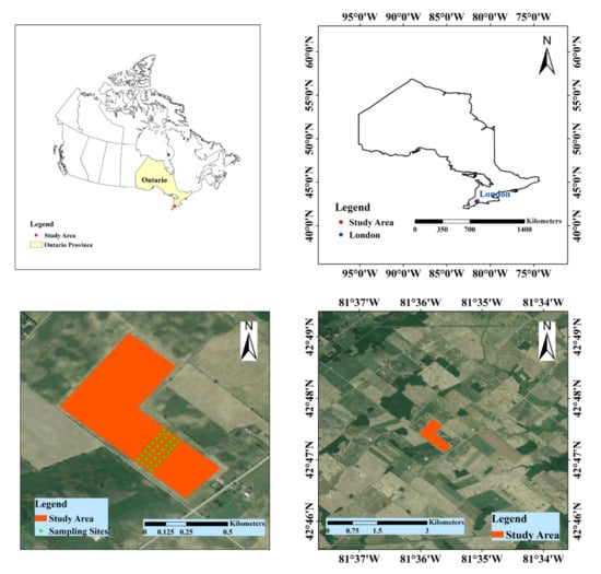
Figure 1.
Location of the study area.
2.2. Data Used
2.2.1. Ground Truth Data Collection
During the growth stage of winter wheat in the study area, we conducted a total of 8 field surveys from May to July in 2019 [49]. The specific sampling date and the measured SMC range on each sampling date are listed in Table 1. Except for the number of sampling points (16) on the last sampling date (July 10), the number of sampling points on the remaining dates was 32, and a total of 240 sampling points were obtained. For the measurement of SMC at each sampling site, the spacing between any adjacent sampling points was at least 30 m. The surface soil moisture was measured using the Theta Probe soil moisture sensor, at a depth of 5 cm. In order to avoid accidental errors, we measured, on average, six times at each sampling point, and took their mean value as the final measured SMC of the sampling point. Meanwhile, real-time kinematic (RTK) was used to record the longitude and latitude information, so that the parameter information corresponding to the sampling point position could be extracted from the geocoded SAR images. The location of the RTK device was 1.5 cm.

Table 1.
Collected SMC details.
2.2.2. RADARSAT-2 Data Collection and Preprocessing
RADARSAT-2 was equipped with a C-band sensor, with a center frequency of approximately 5.4 GHz. The nominal spatial resolution of the RADARSAT-2 images was approximately 8 m. The satellite revisit period was 24 days, and the orbit period was 100.7 min. In this study, we obtained 8 fine quad-polarized RADARSAT-2 images covering the study area, and the image acquisition date was consistent with the sampling date. Table 2 shows the acquisition date and time, as well as the orbit and incidence angles of these 8 SAR images.
Table 2.
Characteristics of collected RADARSAT-2 data.
The preprocessing of RADARSAT-2 data was completed using SNAP 7.0 software, provided by ESA, and included the following steps:
- (1)
- Radiometric calibration: the quad-polarization complex images of backscattering coefficient were generated;
- (2)
- Based on the complex images obtained in step 1, we generated the coherency matrix (T3 matrix);
- (3)
- Polarization filtering: the refined Lee filter was used to reduce the noise generated in step 2, and its window size was set to 7 × 7;
- (4)
- Terrain correction and projection transformation: the filtered data was geocoded with an SRTM-3 digital elevation model, and the output coordinate system was projected to WGS84.
3. Methods
Throughout this study, the Freeman–Durden decomposition technique, optimal roughness parameters, and surface scattering models (e.g., CIEM and Dubois) were used to estimate the SMC across the wheat field in our study area. Figure 2 shows the flowchart of the SMC estimation.
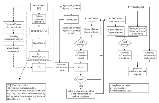
Figure 2.
Workflow of soil moisture retrieval.
- (1)
- RADARSAT-2 data were preprocessed, and T3 matrix was obtained;
- (2)
- Scattering mechanism analysis was used to analyze the main scattering mechanisms of winter wheat in different growth stages in the study area;
- (3)
- The backscattering coefficient of the bare surface was calculated based on the surface scattering matrix (TG). The surface backscattering coefficient and the measured SMC were used to construct the SMC estimation dataset. For each image, we randomly selected 70% as the training set, and the remaining 30% as the validation set. In order to avoid the statistical differences of soil moisture between the training set and the validation set, which would affect the accuracy from the validation set, a selection of statistical characteristics of the training and the validation sets were calculated. Figure 3 shows that the mean, median, and standard deviation of the training and validation sets are significantly close to the statistical characteristics of the total data set, which meets the requirements for data splitting;
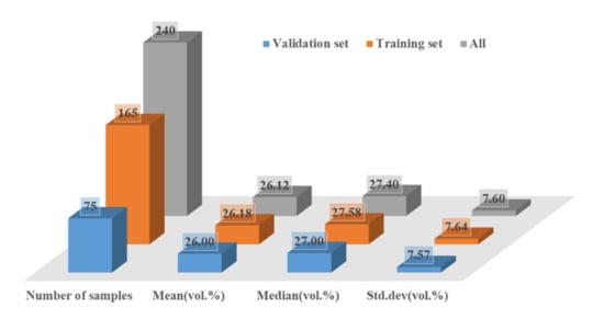 Figure 3. Partial statistical characteristics across the training and validation datasets.
 - (4)
- On the training set, based on the surface backscattering coefficient simulated by the CIEM or the Dubois model under different roughness conditions in a given range, and the surface backscattering coefficient obtained by polarization decomposition, the cost function between them was constructed to estimate the SMC of each sampling point;
- (5)
- The roughness parameters were optimized when the RMSE between the estimated SMC and the measured SMC on the training set was minimized;
- (6)
- The simulated backscattering coefficient from the CIEM or the Dubois model with optimal roughness parameters was obtained, and then a same cost function was constructed between the simulated backscattering coefficient and the backscattering coefficient obtained by polarization decomposition on the validation set. Then, the estimated SMC was retrieved on the validation set, and the accuracy was also verified on the validation set;
- (7)
- The model with the highest accuracy on the validation set was selected to draw the regional SMC map of the winter wheat area.
3.1. Polarimetric Decomposition Methods
3.1.1. Cloude–Pottier Decomposition
Based on the eigenvector analysis of the polarization coherence matrix, Cloude and Pottier propose a decomposition theorem that includes all scattering mechanisms [50]. The coherence matrix is decomposed into the weighted sum of three components, using eigenvalue decomposition, each of which corresponds to a scattering mechanism. By calculating the eigenvalues and eigenvectors from the decomposition, three parameters are obtained: polarization entropy “H”, average scattering angle “α”, and anti-entropy “A”; the values of H and α provide a way to understand the mechanism of scattering [51]. The calculation formulas are as follows:
where is the eigenvalue of coherence matrix T3, and is the eigenvector.
3.1.2. Freeman–Durden Decomposition
Freeman and Durden propose a three-component scattering model based on VanZyl’s research [52]. The main idea of the model is to decompose the polarization coherence matrix (T3) into three main scattering mechanisms, namely, the scattering from the surface (TG), volume scattering from the vegetation canopy (TV), and dihedral scattering (TD) generated by the interaction between the vegetation and the surface. T3 can be decomposed into the following form:
where the “*” represents the conjugate transpose; TG is simulated by the Bragg model: β denotes the normalized difference of the Bragg scattering in H and V polarization, and is the intensity coefficient of the surfaces scatter component matrix; TD is simulated by the Fresnel model, where α is the normalized difference of the combined ground-stalk Fresnel reflection in H and V polarizations, and is the intensity coefficient of the dihedral scatter component matrix; and TV depends on the selected form of the volume scattering matrix ([V]), and the intensity coefficient of [V] (). Yamaguchi proposes three kinds of volume scattering matrices for different vegetation orientations (i.e., vertical, random, and horizontal) according to the Pr value [46,53].
where Tvv, Tvr, and Tvh represent the volume coherence matrix components of vertical, random, and horizontal vegetation orientations, respectively. In this study, the estimation performances of SMC under these three volume scattering matrices were compared.
The power of each scattering component was obtained as follows, based on the decomposition result of T3 [54]; Ps, Pd, and Pv correspond to the power of surface scattering, dihedral scattering, and volume scattering, respectively.
When the dihedral scattering component is ignored, TG is expressed in the following form:
When the volume scattering matrix was selected, the nonnegative eigenvalue decomposition (NNED) method was used to determine the value of [55], which met the condition that the minimum eigenvalue of TG was zero after removing the dihedral scattering component. Based on the coherency matrix corresponding to the surface scattering component, the surface backscattering coefficient was obtained [51,56].
The local incidence of SAR usually has a significant effect on the surface backscattering coefficient, which cannot be ignored in soil moisture estimation. In order to limit the influence of different local incidence angles, the theoretical method proposed by Ulaby et al. [57] was used to reduce the influence of local incidence angles after decomposition:
where θ is the incidence angle, is the reference incidence angle (30°), is the surface backscattering coefficient obtained by polarization decomposition, and is the normalized backscattering coefficient according to the reference incidence angle. In this study, the reference incidence angle was set to 30°.
3.2. Soil Surface Backscattering Modeling
3.2.1. Dubois Model
Dubois et al. [26] establish an empirical scattering model based on multi-frequency, multi-polarization, and multi-angled scatterometer data measured on the ground with different surface roughness [26], and its specific expression is as follows:
The equation above establishes the functional relationship between the backscattering coefficient and surface parameters (e.g., RMS height (s) and soil dielectric constant (ε)), and the sensor configuration parameters (e.g., incident angle (θ) and wavelength (λ)). Where and are the backscattering coefficients of the bare land surface under HH and VV channels simulated by the Dubois model, respectively, k is the free space wavenumber (k = 2π/λ).
The Dubois model is not suitable for the rough surface conditions (ks > 2.5) [58]. Therefore, the RMS height of the lookup table constructed by the Dubois model in this study is between 0–2.2 cm. The SMC was calculated from the ε using the Topp model, shown below [59]:
3.2.2. CIEM Model
The integral equation model (IEM) is a theoretical radar backscatter model with a high validity range [28]. The IEM model establishes the functional relationship between the co-polarized backscattering coefficient and the roughness parameters (correlation length (L), RMS height (s)), dielectric constant, incident angle, and wavelength, etc.). Given the uncertainty of the field measurement of the surface correlation length (L), Baghdadi et al., (2006) establish the semi-empirical relationship between the corrected L and the s, based on abundant SAR images and measured data based on an IEM model, reduce the parameters describing the surface roughness of the soil, and develop a calibrated IEM model (CIEM). The empirical relationship is expressed as [60]:
where L is the corrected correlation length, s is the RMS height, θ represents the incident angle, and pp represents the polarization mode (HH, VV). The coefficients “” and “” are related to the polarization mode, and the coefficients “” and “” are independent of the polarization mode. The specific coefficients of the semi-empirical correction model for C-band SAR data are as follows [60]:
In this study, the RMS height range of the lookup table constructed by CIEM model is consistent with the Dubois model, i.e., 0–2.2 cm.
3.2.3. Optimum Surface Roughness Parameter
Roughness is an important parameter in the surface scattering model, but it is difficult to measure, especially in areas with dense vegetation. Due to the lack of measured roughness parameters in the study area, the surface scattering models cannot be used to simulate the backscattering coefficients of bare soil surface with the actual roughness of sampling points. Therefore, the optimum surface roughness parameter proposed by Bai et al., (2016) [5] was used to parameterize the surface scattering model. This method assumes that the roughness parameter in the study area is a fixed value. SMC is estimated within a certain roughness range. The roughness parameter is taken as the optimum surface roughness parameter of the study area when the RMSE between the estimated SMC values and the measured SMC values is minimized. In this study, only the RMS height is used as the roughness parameter in the surface scattering models.
3.3. Soil Moisture Estimation and Performance Assessment
From the training set, the ground backscattering coefficient () was obtained, using the polarization decomposition. Under different roughness conditions, the lookup table constructed by the Dubois and CIEM models is obtained: the simulated ground backscattering coefficient at different SMC conditions. The following cost function was constructed to estimate SMC:
F (1), F (2), and F (3) represent the cost functions constructed using the VV polarization backscattering coefficient, HH polarization backscattering coefficients, and the combination of VV polarization and HH polarization backscattering coefficients, respectively. When the cost function is minimized, the SMC value corresponding to the backscattering coefficient simulated by the scattering model is taken as the SMC value of the sample point.
The performance of different models was compared and evaluated using statistical indicators, including the coefficient of determination (R2, Equation (13)) and root mean square error (RMSE, Equation (14)). The higher the R2 and the lower the RMSE mean, the better the fitting effect is between the estimated and the measured values, with better model estimation performance and higher accuracy.
where n is the number of sampling points; and represent the measured SMC value and estimated SMC value of the i-th sample site, respectively; and is the mean values of the measured SMC values.
4. Results and Discussion
4.1. Scattering Mechanisms Analysis
The H/α scatter diagram obtained using the Cloude–Pottier decomposition of the pixels of the sampling points in the study area is shown in Figure 4.
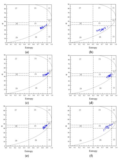
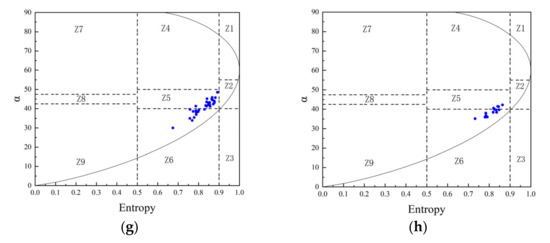
Figure 4.
H and α plots of the wheat fields on sampling dates. (a) 9 May 2019, (b) 16 May 2019, (c) 20 May 2019, (d) 29 May 2019, (e) 2 June 2019, (f) 9 June 2019, (g) 16 June 2019, and (h) 10 July 2019.
As shown in Figure 4, the scatter points of wheat sampling points during the growth period are relatively concentrated in the H/α scatter diagram. The scattered points are distributed primarily among the Z2, Z5, and Z6 areas of the graphs, which indicates that the backscattering composition of the study area is mainly composed of vegetation body scattering, and surface scattering attenuated by vegetation. Therefore, the bare surface scattering model is not directly applied to the soil moisture inversion of wheat-covered farmland. As the wheat grows and develops, its canopy coverage increases gradually, so its volume scattering grows stronger and stronger, which is consistent with the trend that the scattered points show, gradually moving from the Z6 area to the Z5 and Z2 areas. On 16 May, as compared to 9 May, the scattered points are concentrated in the Z6 area, which is due to the incident angle of the SAR image on 16 May being lower than it is on 9 May, and the surface scattering is dominant at a low incident angle [61].
In order to further analyze the scattering mechanism, the percentages of the surface scattering components, the dihedral scattering, and the volume scattering during different phases are obtained based on Freeman–Durden decomposition, as shown in Figure 5. Each point corresponding to the left Y-axis in the figure is obtained by calculating the mean value of different scattering component proportions of all the sampling points in the study area on a certain date. For each sampling date, we calculate the mean value of the volume, surface, and dihedral scattering proportions of all the sampling points. The NDVI in the figure is calculated based on six cloud-free Sentinel-2 images, with acquisition dates near the sampling time. As shown in Figure 5, NDVI first indicate a rapid growth, followed by a slower increase, and then a rapid decrease on the last date. This is consistent with the growth process of winter wheat. The rapid decline in the NDVI on the last sampling date is due to the wheat being fully mature and yellow, resulting in a weakening of the absorption of the red light band, but the coverage of the wheat is still high. On the first two sampling dates, when the NDVI is low, the surface scattering ratio is high, while with the increase in the NDVI, or vegetation cover, the surface scattering ratio decreases significantly. This is consistent with previous studies; the increase in wheat coverage results in more backscattering attenuation [36]. The proportion of scattering components obtained by polarization decomposition is consistent with the growth of the vegetation. The proportion of the dihedral scattering energy is deficient during the wheat growth period, and the backscattering is from both volume scattering and surface scattering. Therefore, ignoring the dihedral scattering component simplifies the calculation of the backscattering coefficient by polarization decomposition, as well as the subsequent estimation of soil moisture. As shown in Figure 5, on 16 May, the surface scattering ratio increases, and the volume scattering ratio decreases, which is consistent with the results shown in Figure 4, due to the influence of the low incidence angle. In general, the proportion of the volume scattering components of wheat in the study area is significantly larger than that of the surface scattering components. Therefore, wheat in growing season has a strong attenuation effect on the total SAR signal, resulting in a relatively low proportion of scattering components reaching the surface.
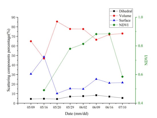
Figure 5.
Energy percentage of three scattering mechanisms and NDVI on different dates.
4.2. Simulated Backscattering Coefficient
Figure 6 illustrates the backscattering coefficients (VV, HH) simulated using the CIEM and Dubois models at a 30° incident angle, with different RMS heights and SMCs. It is evident that the backscattering coefficients simulated by the two surface scattering models increase as the RMS height or SMC content increase. The simulated values of the VV polarization are higher than that of the HH polarization when the roughness and soil moisture content are the same. When the roughness is very low, the two models are not sensitive to the changes in soil moisture. As compared with the CIEM model, the simulated backscattering coefficient of the Dubois model is not sensitive to the change in soil moisture when it is low (SMC < 10 vol.%). However, when the roughness is higher than a certain range, it is very sensitive to the change in soil moisture at a high SMC (SMC greater than 30 vol.% or 40 vol.%). Therefore, when the soil is too dry or too wet, there is uncertainty.
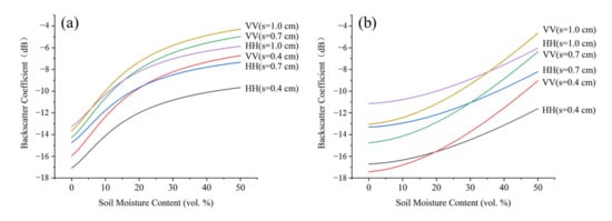
Figure 6.
Simulated backscattering coefficients at different root mean square height and SMC conditions (a) CIEM; (b) Dubois Model.
4.3. CIEM and Dubois Estimation Results
In this study, the dihedral scattering component is ignored due to its low contribution. Different volume scattering matrices (e.g., vertical, random, horizontal, and volume matrix selected according to the Pr value) are selected to compute the surface backscattering coefficient based on polarization decomposition. After solving the surface backscattering coefficients, and combining the scattering models (i.e., CIEM and Dubois), the optimal roughness parameter, and the corresponding cost function, the soil moisture of the validation set is estimated according to the workflow shown in Figure 2. The results are listed in Table 3 and Table 4. The horizontal label in the table represents which cost function in Equation (12) is used, and the vertical label represents which volume scattering matrix selection is used. Furthermore, Table 3 reports the estimated results of the validation set using the CIEM model. When using the fixed volume scattering matrix, including either the vertical, random, or horizontal volume scattering matrix, a relatively high estimation accuracy is obtained on the test set only in the following two cases, as shown in bold in Table 3: when the vertical volume scattering matrix is combined with the cost function F (1), and when horizontal volume scattering matrix is combined with F (2), and the estimation accuracy is R2 = 0.400 and RMSE = 7.02 vol.%; and R2 = 0.360 and RMSE = 8.71 vol.%, respectively. In other cases, including the strategy of dynamically selecting the volume scattering matrix according to the Pr value, the estimation effect on the test set is poor, which suggests a lower R value and a higher RMSE value. Table 4 reports the results of the Dubois model on the validation set, and the same results as the CIEM model are obtained. When the vertical volume scattering matrix is combined with F (1), and the horizontal volume scattering matrix is combined with F (2), a relatively high estimation accuracy is obtained, which are R2 = 0.510 and RMSE = 5.80 vol.%; and R2 = 0.480 and RMSE = 8.00 vol.%, respectively.
Table 3.
Estimation results using CIEM model.
Table 4.
Estimation results using Dubois model.
Figure 7a,b illustrate the field mean of the surface backscattering coefficients of the VV polarization and HH polarization obtained by the polarization decomposition method using the vertical volume scattering matrix and the horizontal volume scattering matrix, respectively. As shown in Figure 7a, the surface backscattering coefficient of the HH polarization is very low, as compared to the VV polarization, which is basically less than −16 dB. Therefore, there is a large estimation error when using the lookup table and cost function constructed under different roughness conditions to estimate soil moisture. For example, when the RMS height is low, the simulated backscattering coefficient is not sensitive to the change in soil moisture, and the estimated SMC is more likely to be larger or smaller than the actual value. When the RMS height exceeds the threshold, the minimum value of the simulated backscattering coefficient exceeds −16 dB, as shown in Figure 6, and, therefore, the soil moisture is significantly underestimated, due to the low backscattering coefficient. Moreover, Figure 7b reflects the same problem; after using the horizontal volume scattering matrix, the value of the surface backscattering coefficient of VV polarization is very low, resulting in a large estimation error. The estimation accuracies of the other two volume scattering matrix selection strategies (i.e., random and Pr-based) are relatively low. However, the calculated surface backscattering coefficient is low as a result of not being within the effective estimation range of the lookup table. Therefore, those two matrix selection strategies are not be suitable for extracting the surface backscattering coefficient of the study area in order to estimate the SMC.
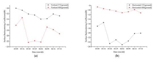
Figure 7.
Mean value of surface backscatter obtained by polarization decomposition (a) Vertical volume scattering matrix; (b) Horizontal volume scattering matrix.
According to the estimation results of the validation set, the two scattering models obtain better estimation performances for the VV surface backscattering coefficient calculated based on the vertical volume scattering matrix, and the HH surface backscattering coefficient calculated based on the horizontal volume scattering matrix. Therefore, these two scattering components are regarded as effective surface backscattering coefficients. Therefore, we combine the two effective surface scattering components, and then estimate the soil moisture of the validation set based on the optimal roughness parameter and the cost function F (3) in Equation (12); the results are shown in Figure 8.
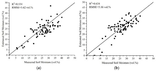
Figure 8.
Scatter plot between measured and estimated soil moisture using F (3) based on effective surface scattering of VV and HH (a) CIEM; (b) Dubois models.
As shown in Figure 8, the accuracy of combining the VV and HH effective backscattering components is higher than using only one of them on the validation set: the accuracy of the CIEM model is R2 = 0.534 and RMSE = 5.62 vol.%, and the accuracy of the Dubois model is R2 = 0.634 and RMSE = 5.16 vol.%. This is likely due to the combination of the HH and VV effective surface scattering that contains more backscattering information than a single polarization, which reduces the estimation error of the scattering model under the optimal roughness parameters. Overall, the estimation performance of the Dubois model is better than that of the CIEM model. To show a further comparison of the differences between the two models, Figure 9 displays the estimation accuracy (RMSE) of the CIEM and Dubois models on different sampling dates. As shown in Figure 9, the accuracy of the Dubois model estimation is generally better than that of the CIEM model on seven sampling dates, from 9 May to 16 June. Specifically, the RMSE is close to, or lower than, that of the CIEM. However, on the last sampling date, the accuracy of the Dubois model is significantly lower than that of the CIEM model. This is due to the SMC at the sampling point on 10 July being low (the average is less than 10 vol.%). As shown in Figure 6, when the SMC is low, the backscattering coefficient simulated by the Dubois model is not sensitive to the change in soil moisture, so there is a large estimation error.
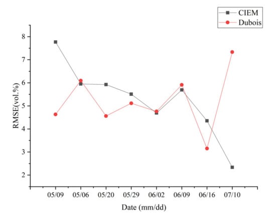
Figure 9.
Estimation accuracy of CIEM and Dubois models on different sampling dates.
4.4. SMC Dynamics during Wheat Growing Seasons
The dynamic changes in the measured and estimated values on different dates in the validation set when the CIEM or Dubois model is applied to achieve the best SMC estimation performance are shown in Figure 10. The estimated SMC can better restore the change trend of measured soil moisture. There is no artificial irrigation for wheat in the study area, so the SMC is only affected by precipitation, vegetation absorption, and soil evapotranspiration. In order to better explain the SMC temporal variability in Figure 10 and the soil moisture maps, the rainfall data in the study area is obtained from the ERA5-Land dataset (https://www.ecmwf.int/ (accessed on 20 December 2021)). ERA5-Land provides a consistent view of the water and energy cycles at the surface level for several decades. It contains a detailed record from the year 1950 onwards, with a temporal resolution of 1 h. The native spatial resolution of the ERA5-Land reanalysis dataset is 9 km on a reduced Gaussian grid. The daily precipitation from 1 May to 10 July in the study area is shown in Figure 10.
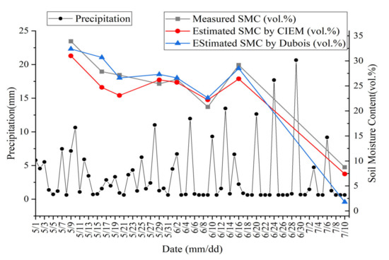
Figure 10.
Dynamics of daily precipitation and mean SMC.
As shown in Figure 10, there is obvious precipitation in the two days prior to 9 May. In addition, the wheat plants are sparse, and water absorption is low, so the SMC on 9 May is high. From 16 May to 2 June, the mean values of SMC are roughly the same. This is most likely due to less rainfall. The soil moisture supplemented by rainfall reaches a dynamic balance with the soil water absorbed by wheat and consumed by soil evapotranspiration. There is also obvious heavy precipitation on 2 June, but the soil moisture does not increase significantly. This is due to the precipitation time occurring after the sampling was completed. From 2 June to 16 June, the mean SMC first decreases and then increases, probably due to the difference in precipitation near the sampling date. On the last sampling date, the soil moisture is the lowest, which could be due to the high temperatures in July, the strong soil evapotranspiration, and the lack of precipitation a few days before sampling.
4.5. Variation and Analysis of Optimal Roughness Parameters
In order to verify whether the optimal roughness parameter adjusts the estimation accuracy of soil moisture, and the feasibility of parameterized surface scattering models, a time-series dynamic variation of the optimal roughness parameter is obtained. The roughness parameters of the scattering model used in this study are the RMS height of the soil surface. According to the above estimation results, it is found that better estimation performance is obtained under the following scattering component conditions: (1) an effective VV scattering component, (2) an effective HH scattering component, and (3) a combination of the VV and HH scattering components. Therefore, Figure 11 shows the variation of the optimal roughness parameter (RMS height) when estimating soil moisture under the above three conditions. The estimation results of the two scattering models indicate that the RMS height first presents a decreasing trend, and then increases. The RMS heights on the first and last days are higher than those on the other days. For each sampling date, the RMS height based on the VV effective scattering component is the largest, the RMS height based on the HH effective scattering component is the smallest, and the RMS height based on the combination of VV and HH is somewhere between the first two.
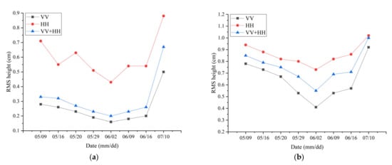
Figure 11.
Time series variation of effective roughness parameters (a) CIEM; (b) Dubois Model.
Figure 12 shows the mean values of effective surface scattering and measured soil moisture on different sampling dates. We find that the HH effective surface scattering component based on polarization decomposition is higher than the VV effective surface scattering component. As shown in Figure 6, when the RMS height is constant, the VV polarization backscattering coefficient simulated by the models is greater than the HH polarization backscattering coefficient simulated by the CIEM or the Dubois model. Due to the simulated backscattering coefficient having a positive correlation with the roughness parameters, when the simulated value is close to the effective scattering component value, higher effective roughness parameters are obtained using HH polarization. Among all the sampling dates, the SMC mean value on 9 May is the highest. As shown in Figure 6, when the SMC is constant, the simulated backscattering coefficient is positively correlated with the RMS height. When the RMSE between the estimated SMC and the measured SMC is the smallest, and the backscattering coefficient difference between the two dates is small, a higher RMS height is obtained when the SMC is large. Therefore, the optimal roughness parameters obtained on 9 May are higher. The average SMC on 10 July is the lowest, which is less than 10 vol.%. When the effective surface scattering component hardly changes, in order to obtain a lower SMC value, the corresponding RMS height value increases, which also indicates why the optimal roughness parameter is high on 10 July.
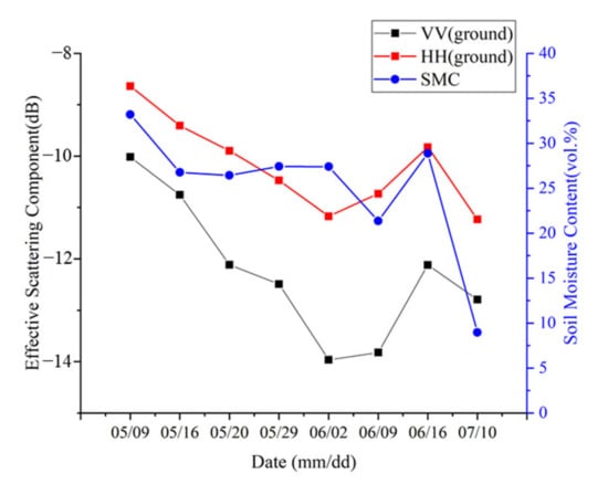
Figure 12.
Mean value of effective surface scattering and mean value of measured soil moisture.
Taking the CIEM model as an example, Figure 13 illustrates the cost function values obtained based on different effective surface scattering components at one sampling point on 9 May, when the RMS height is 0.29 cm and 0.89 cm. F1, F2, and F3, respectively, correspond to the cost function in Equation (12), and use the corresponding effective scattering component (VV, HH, VV + HH). The horizontal axis represents the SMC. When different cost functions are used, the SMC corresponding to the minimum value is taken as the estimated soil moisture at this sampling point. As shown in Figure 13, when F1, F2, and F3 obtain minimum values, the SMC value corresponding to F3 is between the SMC corresponding to F1 and F2. Moreover, with the increase in roughness, the SMC corresponding to the minimum of the three cost functions decreases. Therefore, when the estimated soil moisture value using different cost functions is close to the actual value (F1_min ≈ F2_min ≈ F3_min), the RMS height obtained by combining the VV and HH effective scattering components is between the RMS heights obtained using a single effective scattering component. In conclusion, it proves that the optimal roughness parameter can be used as an empirical coefficient of the surface scattering models, in order to adjust the estimation accuracy of soil moisture. Therefore, in the absence of measured roughness parameters, it is feasible to use the optimal roughness parameter to parameterize the surface scattering model for the soil moisture estimation method in this study.
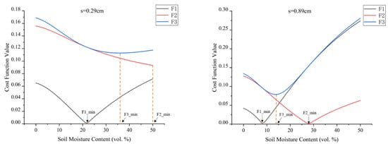
Figure 13.
Values of three cost functions under different roughness conditions.
4.6. Soil Moisture Map
Based on these results, an optimal soil water estimation model is employed, combining the effective surface scattering components VV and HH to complete the mapping of the SMC in the study area, as shown in Figure 14. Figure 14a,b are maps using the CIEM and Dubois models as surface scattering models, respectively. Compared to the measured mean value of soil moisture, the soil moisture map agrees with the measured values. For example, Figure 12 shows that the soil moisture of the sampling points on 16 June is lower than that of the two adjacent sampling dates, seen in Figure 14. When comparing the soil moisture maps under two scattering models, the CIEM soil moisture map and the Dubois soil moisture map are generally consistent in the high- and low-value soil moisture areas. The soil moisture in the study area shows significantly high and low value distribution rather than uniform distribution, which may be due to two factors. First, the terrain of the study area is not flat and has some slope, resulting in an uneven soil moisture distribution. Second, the growth of wheat and the soil moisture absorption in different regions are not the same. Taking the Dubois-SMC map as a reference, the low-value area on the Dubois-SMC map is orange or red, and its value is lower than the same area on the CIEM-SMC map. The high-value area on the CIEM-SMC map is green in color, and its value is higher than the same area on the Dubois-SMC map. Except for the last sampling date, the patch area of the low-value area on the Dubois-SMC map is also smaller than the low-value area on the CIEM-SMC map. When combined with Figure 6 and Figure 11, we find that, except for the last sampling date, when constructing the lookup table of the surface scattering model based on the optimal roughness, the backscattering coefficient simulated by the CIEM model is not sensitive to the change in soil moisture, as compared to the Dubois model. Therefore, the comparison between the dry area and the wet area in the CIEM-SMC diagram is not apparent, as compared to the Dubois-SMC diagram. On the last sampling date, the Dubois-SMC map shows a large area of zero value. The main reason is that when the soil moisture is low, the Dubois model is not sensitive to the change in soil moisture, resulting in a significant underestimation of the SMC. Therefore, the Dubois model is not suitable for the estimation of the soil moisture over dry areas.
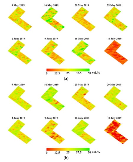
Figure 14.
Soil moisture map for the study area (a) CIEM-SMC map; (b) Dubois-SMC map.
The range of the soil moisture is large (0–50 vol.%), which is an obvious deviation from the actual situation. This is attributed to the use of optimal roughness parameterized scattering models in this study. For each sampling date, using the optimal roughness parameter to characterize the roughness conditions of all sampling points adjusts the estimation accuracy of soil moisture as a whole, but it has limitations. For example, when the optimal roughness parameter is far less than the actual roughness parameter, the estimated value based on the optimal roughness parameter is significantly overestimated when using the same surface backscattering coefficient. An estimate of 50 vol.% above the critical value occurs. According to Table 1, the range of measured soil moisture is relatively large. The soil moisture of most pixels in the study area is accurately estimated, but the soil moisture estimated based on the optimal roughness parameters is overestimated and underestimated in some pixels. Therefore, the SMC in the figures ranges from 0 to 50 vol.%.
4.7. Limitation and Potential Improvements
Although this study provides a good estimation performance for the SMC in the study area, it has some limitations that should be improved in future research. Firstly, the measured data in the field only includes part of the wheat growth period. In future, it is necessary to collect and analyze the measured soil moisture for the entire growing season to evaluate the effective range of the proposed method. Secondly, the proposed method captures the dynamic changes of soil moisture in the study area. However, this is the result of constructing the model based on the sampling points in the study area. For the applicability of the final model, constructed based on a specific area, to estimate the soil moisture content of other wheat fields, or the same field in the same growing stage but in different years, it needs further verification in future research. Thirdly, volume scattering is the main scattering component for the wheat field in this study, but only a relatively simple volume scattering matrix is used in our study. Therefore, it is necessary to explore a complicated volume scattering matrix, or a surface scattering component extraction method, in future. In addition, this study focuses on wheat crops. Consequently, this method should also be tested on other crops, to validate its generalizability.
5. Conclusions
In this study, based on RADARSAT-2 fully polarized data and polarization decomposition, the surface backscattering coefficients with different volume scattering matrices were extracted. The SMC of the wheat fields was estimated by combining surface scattering models, optimal roughness parameters, and three cost functions. From our experiment, we drew the following conclusions:
- (1)
- Based on the H/α decomposition and the Freeman–Durden decomposition, the scattering components in the study area are mainly volume scattering component and surface scattering component.
- (2)
- The surface backscattering coefficients were extracted using four volume scattering matrix selection strategies (i.e., horizontal, vertical, random, and based on the Pr value), and combined with the optimal roughness parameters; then the CIEM and Dubois models, as well as different cost functions, were used to retrieve the SMC. Finally, we found that the VV scattering component, based on the vertical volume scattering matrix, and the HH volume scattering component, based on the horizontal volume scattering matrix, achieve the best performance. Using these two scattering components as the effective surface scattering components of VV and HH, combined with the cost function F (3), the highest estimation accuracy is obtained.
- (3)
- From the optimal soil moisture estimation model, the spatial distribution map of SMC in the winter wheat region was completed.
This study achieves encouraging results. Once the limitations are addressed, it has the potential to be an effective means for the remote monitoring of soil moisture in winter wheat farmland, and may be used as a basis to diagnose the health status of farmland.
Author Contributions
Data curation, L.C. and M.X. (Minfeng Xing); investigation, L.C., M.X. (Minfeng Xing) and B.H.; methodology, L.C. and M.X. (Minfeng Xing); supervision, M.X. (Minfeng Xing) and J.W.; validation, L.C. and M.X. (Minfeng Xing); writing—original draft, L.C.; writing—review & editing, M.X. (Minfeng Xing), B.H., J.W., M.X. (Min Xu), Y.S. and X.H. All authors have read and agreed to the published version of the manuscript.
Funding
This work was supported by the National Natural Science Foundation of China, grant number 41601373; Sichuan Science and Technology Program, grant number 2020YFG0048; the Canadian Space Agency SOAR-E program, grant number SOAR-E-5489; the Scientific Research Starting Foundation from Yangtze Delta Region Institute (Huzhou), University of Electronic Science and Technology of China, grant number U03210022; and the Fundamental Research Funds for the Central Universities, grant number ZYGX2019J070.
Conflicts of Interest
The authors declare no conflict of interest.
References
- Seneviratne, S.I.; Corti, T.; Davin, E.L.; Hirschi, M.; Jaeger, E.B.; Lehner, I.; Orlowsky, B.; Teuling, A.J. Investigating soil moisture-climate interactions in a changing climate: A review. Earth-Sci. Rev. 2010, 99, 125–161. [Google Scholar] [CrossRef]
- Kornelsen, K.C.; Coulibaly, P. Advances in soil moisture retrieval from synthetic aperture radar and hydrological applications. J. Hydrol. 2013, 476, 460–489. [Google Scholar] [CrossRef]
- Mccoll, K.A.; Alemohammad, S.H.; Akbar, R.; Konings, A.G.; Yueh, S.; Entekhabi, D. The global distribution and dynamics of surface soil moisture. Nat. Geosci. 2017, 10, 100–104. [Google Scholar] [CrossRef]
- Kolassa, J.; Reichle, R.H.; Liu, Q.; Alemohammad, S.H.; Walker, J.P. Estimating surface soil moisture from SMAP observations using a Neural Network technique. Remote Sens. Environ. 2018, 204, 43–59. [Google Scholar] [CrossRef]
- Bai, X.J.; He, B.B.; Li, X.W. Optimum Surface Roughness to Parameterize Advanced Integral Equation Model for Soil Moisture Retrieval in Prairie Area Using Radarsat-2 Data. IEEE Trans. Geosci. Remote Sens. 2016, 54, 2437–2449. [Google Scholar] [CrossRef]
- Xing, M.F.; He, B.B.; Ni, X.L.; Wang, J.F.; An, G.Q.; Shang, J.L.; Huang, X.D. Retrieving Surface Soil Moisture over Wheat and Soybean Fields during Growing Season Using Modified Water Cloud Model from Radarsat-2 SAR Data. Remote Sens. 2019, 11, 1956. [Google Scholar] [CrossRef] [Green Version]
- Wang, Q.; Li, J.C.; Jin, T.Y.; Chang, X.; Zhu, Y.C.; Li, Y.W.; Sun, J.J.; Li, D.W. Comparative Analysis of Landsat-8, Sentinel-2, and GF-1 Data for Retrieving Soil Moisture over Wheat Farmlands. Remote Sens. 2020, 12, 2708. [Google Scholar] [CrossRef]
- Shi, H.; Zhao, L.; Yang, J.; Lopez-Sanchez, J.M.; Zhao, J.; Sun, W.; Shi, L.; Li, P. Soil moisture retrieval over agricultural fields from L-band multi-incidence and multitemporal PolSAR observations using polarimetric decomposition techniques. Remote Sens. Environ. 2021, 261, 112485. [Google Scholar] [CrossRef]
- Serrano, D.; Vila, E.; Barrios, M.; Darghan, A.; Lobo, D. Surface Soil Moisture Monitoring with Near-Ground Sensors: Performance Assessment of a Matric Potential-Based Method. Measurement 2020, 155, 107542. [Google Scholar] [CrossRef]
- Ochsner, T.E.; Cosh, M.H.; Zreda, M.G.; Cuenca, R.H.; Dorigo, W.; Draper, C.S.; Hagimoto, Y.; Kerr, Y.H.; Larson, K.M.; Njoku, E.G. State of the Art in Large-Scale Soil Moisture Monitoring. Soil Sci. Soc. Am. J. 2013, 77, 1888–1919. [Google Scholar] [CrossRef] [Green Version]
- Tripathi, A.; Tiwari, R.K. Synergetic utilization of sentinel-1 SAR and sentinel-2 optical remote sensing data for surface soil moisture estimation for Rupnagar, Punjab, India. Geocarto. Int. 2020, 1–22. [Google Scholar] [CrossRef]
- Kumar, P.; Prasad, R.; Choudhary, A.; Gupta, D.K.; Mishra, V.N.; Vishwakarma, A.K.; Singh, A.K.; Srivastava, P.K. Comprehensive evaluation of soil moisture retrieval models under different crop cover types using C-band synthetic aperture radar data. Geocarto Int. 2019, 34, 1022–1041. [Google Scholar] [CrossRef]
- Aubert, M.; Baghdadi, N.N.; Zribi, M.; Ose, K.; El Hajj, M.; Vaudour, E.; Gonzalez-Sosa, E. Toward an Operational Bare Soil Moisture Mapping Using TerraSAR-X Data Acquired Over Agricultural Areas. IEEE J. Sel. Top. Appl. Earth Obs. Remote Sens. 2013, 6, 900–916. [Google Scholar] [CrossRef]
- El Hajj, M.; Baghdadi, N.; Zribi, M.; Bazzi, H. Synergic Use of Sentinel-1 and Sentinel-2 Images for Operational Soil Moisture Mapping at High Spatial Resolution over Agricultural Areas. Remote Sens. 2017, 9, 1292. [Google Scholar] [CrossRef] [Green Version]
- Jackson, T.J.; Cosh, M.H.; Bindlish, R.; Starks, P.J.; Bosch, D.D.; Seyfried, M.; Goodrich, D.C.; Moran, M.S.; Du, J.Y. Validation of Advanced Microwave Scanning Radiometer Soil Moisture Products. IEEE Trans. Geosci. Remote Sens. 2010, 48, 4256–4272. [Google Scholar] [CrossRef]
- Tomer, S.K.; Al Bitar, A.; Sekhar, M.; Zribi, M.; Bandyopadhyay, S.; Sreelash, K.; Sharma, A.K.; Corgne, S.; Kerr, Y. Retrieval and Multi-scale Validation of Soil Moisture from Multi-temporal SAR Data in a Semi-Arid Tropical Region. Remote Sens. 2015, 7, 8128–8153. [Google Scholar] [CrossRef] [Green Version]
- Narvekar, P.S.; Entekhabi, D.; Kim, S.B.; Njoku, E.G. Soil Moisture Retrieval Using L-Band Radar Observations. IEEE Trans. Geosci. Remote Sens. 2015, 53, 3492–3506. [Google Scholar] [CrossRef]
- De Keyser, E.; Vernieuwe, H.; Lievens, H.; Alvarez-Mozos, J.; De Baets, B.; Verhoest, N.E.C. Assessment of SAR-retrieved soil moisture uncertainty induced by uncertainty on modeled soil surface roughness. Int. J. Appl. Earth Obs. Geoinf. 2012, 18, 176–182. [Google Scholar] [CrossRef]
- Wagner, W.; Hahn, S.; Kidd, R.; Melzer, T.; Bartalis, Z.; Hasenauer, S.; Figa-Saldana, J.; De Rosnay, P.; Jann, A.; Schneider, S.; et al. The ASCAT Soil Moisture Product: A Review of its Specifications, Validation Results, and Emerging Applications. Meteorol. Z. 2013, 22, 5–33. [Google Scholar] [CrossRef] [Green Version]
- Petropoulos, G.P.; Ireland, G.; Barrett, B. Surface soil moisture retrievals from remote sensing: Current status, products & future trends. Phys. Chem. Earth 2015, 83, 36–56. [Google Scholar] [CrossRef]
- Liu, C.A.; Chen, Z.X.; Shao, Y.; Chen, J.S.; Hasi, T.; Pan, H.Z. Research advances of SAR remote sensing for agriculture applications: A review. J. Integr. Agric. 2019, 18, 506–525. [Google Scholar] [CrossRef] [Green Version]
- Baghdadi, N.; Holah, N.; Zribi, M. Soil moisture estimation using multi-incidence and multi-polarization ASAR data. Int. J. Remote Sens. 2006, 27, 1907–1920. [Google Scholar] [CrossRef]
- Bousbih, S.; Zribi, M.; El Hajj, M.; Baghdadi, N.; Lili-Chabaane, Z.; Gao, Q.; Fanise, P. Soil Moisture and Irrigation Mapping in A Semi-Arid Region, Based on the Synergetic Use of Sentinel-1 and Sentinel-2 Data. Remote Sens. 2018, 10, 1953. [Google Scholar] [CrossRef] [Green Version]
- El Hajj, M.; Baghdadi, N.; Zribi, M. Comparative analysis of the accuracy of surface soil moisture estimation from the C- and L-bands. Int. J. Appl. Earth Obs. Geoinf. 2019, 82, 101888. [Google Scholar] [CrossRef]
- Oh, Y.; Sarabandi, K.; Ulaby, F.T. An Empirical-Model and an Inversion Technique for Radar Scattering From Bare Soil Surfaces. IEEE Trans. Geosci. Remote Sens. 1992, 30, 370–381. [Google Scholar] [CrossRef]
- Dubois, P.C.; Vanzyl, J.; Engman, T. Measuring Soil-Moisture with Imaging Radars. IEEE Trans. Geosci. Remote Sens. 1995, 33, 915–926. [Google Scholar] [CrossRef] [Green Version]
- Baghdadi, N.; Choker, M.; Zribi, M.; El Hajj, M.; Paloscia, S.; Verhoest, N.E.C.; Lievens, H.; Baup, F.; Mattia, F. A New Empirical Model for Radar Scattering from Bare Soil Surfaces. Remote Sens. 2016, 8, 920. [Google Scholar] [CrossRef] [Green Version]
- Fung, A.K.; Li, Z.Q.; Chen, K.S. Backscattering From a Randomly Rough Dielectric Surface. IEEE Trans. Geosci. Remote Sens. 1992, 30, 356–369. [Google Scholar] [CrossRef]
- Ali, I.; Greifeneder, F.; Stamenkovic, J.; Neumann, M.; Notarnicola, C. Review of Machine Learning Approaches for Biomass and Soil Moisture Retrievals from Remote Sensing Data. Remote Sens. 2015, 7, 16398–16421. [Google Scholar] [CrossRef] [Green Version]
- Zhang, X.; Chen, B.Z.; Fan, H.D.; Huang, J.L.; Zhao, H. The Potential Use of Multi-Band SAR Data for Soil Moisture Retrieval over Bare Agricultural Areas: Hebei, China. Remote Sens. 2016, 8, 7. [Google Scholar] [CrossRef] [Green Version]
- Tong, C.; Wang, H.Q.; Magagi, R.; Goita, K.; Zhu, L.Y.; Yang, M.Y.; Deng, J.S. Soil Moisture Retrievals by Combining Passive Microwave and Optical Data. Remote Sens. 2020, 12, 3173. [Google Scholar] [CrossRef]
- Bryant, R.; Moran, M.S.; Thoma, D.P.; Holifield Collins, C.D.; Skirvin, S.; Rahman, M. Measuring Surface Roughness Height to Parameterize Radar Backscatter Models for Retrieval of Surface Soil Moisture. IEEE Geosci. Remote Sens. Lett. 2007, 4, 137–141. [Google Scholar] [CrossRef]
- Su, Z.; Troch, P.A.; De Troch, F.P. Remote sensing of bare surface soil moisture using EMAC/ESAR data. Int. J. Remote Sens. 1997, 18, 2105–2124. [Google Scholar] [CrossRef]
- Baghdadi, N.; King, C.; Bonnifait, A. An empirical calibration of the integral equation model based on SAR data and soil parameters measurements. Int. J. Remote Sens. 2002, 23, 4325–4340. [Google Scholar] [CrossRef]
- El Hajj, M.; Baghdadi, N.; Wigneron, J.P.; Zribi, M.; Albergel, C.; Calvet, J.C.; Fayad, I. First Vegetation Optical Depth Mapping from Sentinel-1 C-band SAR Data over Crop Fields. Remote Sens. 2019, 11, 2769. [Google Scholar] [CrossRef] [Green Version]
- Nasrallah, A.; Baghdadi, N.; El Hajj, M.; Darwish, T.; Belhouchette, H.; Faour, G.; Darwich, S.; Mhawej, M. Sentinel-1 Data for Winter Wheat Phenology Monitoring and Mapping. Remote Sens. 2019, 11, 2228. [Google Scholar] [CrossRef] [Green Version]
- Bazzi, H.; Baghdadi, N.; Fayad, I.; Charron, F.; Zribi, M.; Belhouchette, H. Irrigation Events Detection over Intensively Irrigated Grassland Plots Using Sentinel-1 Data. Remote Sens. 2020, 12, 4058. [Google Scholar] [CrossRef]
- El Hajj, M.; Baghdadi, N.; Zribi, M.; Belaud, G.; Cheviron, B.; Courault, D.; Charron, F. Soil moisture retrieval over irrigated grassland using X-band SAR data. Remote Sens. Environ. 2016, 176, 202–218. [Google Scholar] [CrossRef] [Green Version]
- Attema, E.; Ulaby, F.T. Vegetation modeled as a water cloud. Radio Sci. 1978, 13, 357–364. [Google Scholar] [CrossRef]
- Kumar, K.; Rao, H.S.; Arora, M.K. Study of water cloud model vegetation descriptors in estimating soil moisture in Solani catchment. Hydrol. Processes 2015, 29, 2137–2148. [Google Scholar] [CrossRef]
- Cloude, S.R.; Pottier, E. A review of target decomposition theorems in radar polarimetry. IEEE Trans. Geosci. Remote Sens. 1996, 34, 498–518. [Google Scholar] [CrossRef]
- Baghdadi, N.; Cresson, R.; El Hajj, M.; Ludwig, R.; La Jeunesse, I. Estimation of soil parameters over bare agriculture areas from C-band polarimetric SAR data using neural networks. Hydrol. Earth Syst. Sci. 2012, 16, 1607–1621. [Google Scholar] [CrossRef] [Green Version]
- Baghdadi, N.; Cresson, R.; Pottier, E.; Aubert, M.; Zribi, M.; Jacome, A.; Benabdallah, S. A Potential Use for the C-Band Polarimetric SAR Parameters to Characterize the Soil Surface over Bare Agriculture Fields. IEEE Trans. Geosci. Remote Sens. 2012, 50, 3844–3858. [Google Scholar] [CrossRef]
- Baghdadi, N.; Dubois-Fernandez, P.; Dupuis, X.; Zribi, M. Sensitivity of Main Polarimetric Parameters of Multifrequency Polarimetric SAR Data to Soil Moisture and Surface Roughness Over Bare Agricultural Soils. IEEE Geosci. Remote Sens. Lett. 2013, 10, 731–735. [Google Scholar] [CrossRef] [Green Version]
- Wang, H.; Magagi, R.; Goita, K. Comparison of Different Polarimetric Decompositions for Soil Moisture Retrieval over Vegetation Covered Agricultural Area. Remote Sens. Environ. 2017, 199, 120–136. [Google Scholar] [CrossRef]
- Hajnsek, I.; Jagdhuber, T.; Schcon, H.; Papathanassiou, K.P. Potential of Estimating Soil Moisture under Vegetation Cover by Means of PolSAR. IEEE Trans. Geosci. Remote Sens. 2009, 47, 442–454. [Google Scholar] [CrossRef] [Green Version]
- Jagdhuber, T.; Hajnsek, I.; Bronstert, A.; Papathanassiou, K.P. Soil Moisture Estimation under Low Vegetation Cover Using a Multi-Angular Polarimetric Decomposition. IEEE Trans. Geosci. Remote Sens. 2013, 51, 2201–2215. [Google Scholar] [CrossRef]
- Wang, H.; Ramata, M.; Kalifa, G. Potential of a two-component polarimetric decomposition at C-band for soil moisture retrieval over agricultural fields. Remote Sens. Environ. 2018, 217, 38–51. [Google Scholar] [CrossRef]
- Chen, L.; Xing, M.F.; He, B.B.; Wang, J.F.; Shang, J.L.; Huang, X.D.; Xu, M. Estimating Soil Moisture Over Winter Wheat Fields During Growing Season Using Machine-Learning Methods. IEEE J. Sel. Top. Appl. Earth Obs. Remote Sens. 2021, 14, 3706–3718. [Google Scholar] [CrossRef]
- Cloude, S.R.; Pottier, E. An entropy based classification scheme for land applications of polarimetric SAR. IEEE Trans. Geosci. Remote Sens. 1997, 35, 68–78. [Google Scholar] [CrossRef]
- Lee, J.S.; Pottier, E. Polarimetric Radar Imaging: From Basics to Applications; CRC Press: Boca Raton, FL, USA, 2009. [Google Scholar]
- Freeman, A.; Durden, S.L. A three-component scattering model for polarimetric SAR data. IEEE Trans. Geosci. Remote Sens. 1998, 36, 963–973. [Google Scholar] [CrossRef] [Green Version]
- Yamaguchi, Y.; Moriyama, T.; Ishido, M.; Yamada, H. Four-component scattering model for polarimetric SAR image decomposition. IEEE Trans. Geosci. Remote Sens. 2005, 43, 1699–1706. [Google Scholar] [CrossRef]
- An, W.T.; Cui, Y.; Yang, J. Three-Component Model-Based Decomposition for Polarimetric SAR Data. IEEE Trans. Geosci. Remote Sens. 2010, 48, 2732–2739. [Google Scholar] [CrossRef]
- Van Zyl, J.J.; Arii, M.; Kim, Y. Model-Based Decomposition of Polarimetric SAR Covariance Matrices Constrained for Nonnegative Eigenvalues. IEEE Trans. Geosci. Remote Sens. 2011, 49, 3452–3459. [Google Scholar] [CrossRef]
- Xiao, T.; Xing, M.; He, B.; Wang, J.; Ni, X. Retrieving Soil Moisture over Soybean Fields during Growing Season through Polarimetric Decomposition. IEEE J. Sel. Top. Appl. Earth Obs. Remote Sens. 2020, 14, 1132–1145. [Google Scholar] [CrossRef]
- Ulaby, F.T.; Sarabandi, K.; Mcdonald, K.; Whitt, M.; Dobson, M.C. Michigan microwave canopy scattering model. Int. J. Remote Sens. 1990, 11, 1223–1253. [Google Scholar] [CrossRef]
- Alvarez-Mozos, J.; Gonzalez-Audicana, M.; Casali, J. Evaluation of empirical and semi-empirical backscattering models for surface soil moisture estimation. Can. J. Remote Sens. 2007, 33, 176–188. [Google Scholar] [CrossRef]
- Topp, G.C.; Davis, J.L.; Annan, A.P. Electromagnetic determination of soil water content: Measurements in coaxial transmission lines. Water Resour. Res. 1980, 16, 574–582. [Google Scholar] [CrossRef] [Green Version]
- Baghdadi, N.; Holah, N.; Zribi, M. Calibration of the Integral Equation Model for SAR data in C-band and HH and VV polarizations. Int. J. Remote Sens. 2006, 27, 805–816. [Google Scholar] [CrossRef]
- Wang, H.Q.; Magagi, R.; Goita, K.; Jagdhuber, T.; Hajnsek, I. Evaluation of Simplified Polarimetric Decomposition for Soil Moisture Retrieval over Vegetated Agricultural Fields. Remote Sens. 2016, 8, 142. [Google Scholar] [CrossRef] [Green Version]
Publisher’s Note: MDPI stays neutral with regard to jurisdictional claims in published maps and institutional affiliations. |
© 2022 by the authors. Licensee MDPI, Basel, Switzerland. This article is an open access article distributed under the terms and conditions of the Creative Commons Attribution (CC BY) license (https://creativecommons.org/licenses/by/4.0/).