Abstract
Understorey evaluation is essential in wildlife habitat management, biomass storage and wildfire suppression, among other areas. The lack of a standardised methodology in the field measurements, and in their subsequent analysis, forces researchers to look for procedures that effectively extract understorey data to make management decisions corresponding to actual stand conditions. In this sense, when analysing the understorey characteristics from LiDAR data, it is very usual to ask: “what value should we set the understorey height range to?” It is also usual to answer by setting a numeric value on the basis of previous research. Against that background, this research aims to identify the optimal height to canopy base (HCB) filter–LiDAR metric relationship for estimating understorey height (UH) and understorey cover (UC) using LiDAR data in the Pokupsko Basin lowland forest complex (Croatia). First, several HCB values per plot were obtained from field data (measured HCBi—HCBM-i, where i ϵ (minimum, maximum, mean, percentiles)), and then they were modelled based on LiDAR metrics (estimated HCBi—HCBE-i). These thresholds, measured and estimated HCBi per plot, were used as point cloud filters to estimate understorey parameters directly on the point cloud located under the canopy layer. In this way, it was possible to predict the UH with errors (RMSE) between 0.90 and 2.50 m and the UC with errors (RMSE) between 8.8 and 18.6 in cover percentage. Finally, the sensitivity analysis showed the HCB filter (the upper threshold to select the understorey LiDAR points) is the most important factor affecting the UH estimates, while this factor and the LiDAR metric are the most important factors affecting the UC estimates.
1. Introduction
The concept of forest structure refers to the three-dimensional (3D) distribution of all the elements that configure a forest stand, including species type, size, ages, variety, height strata and others [1]. Most of the research describing 3D vertical structure properties is focused on the tree layer, i.e., overstorey layer [2,3,4], but not the understorey, defined as all the woody vegetation and suppressed trees growing beneath the forest canopy [5,6]. This structural information is transcendent to guide a silvicultural program designed to promote the development of forests with more diverse structures and composition [7]. However, the lack of spatially explicit 3D structure data in forests, specifically for the understorey layer, is a major challenge for ecological management. In addition, understorey vegetation knowledge is crucial for wildlife habitat and biodiversity [8,9], rainfall interceptions in watersheds [10], fire behaviour [11] and understanding forest competition dynamics [12].
The direct field-based methods for measurements of understorey vegetation, such as visual estimations or point-intercept sampling, have an acceptable accuracy, but they are costly and labour intensive, which limits their application to small areas [5,13]. For more than three decades, light detection and ranging (LiDAR), an active remote-sensing technology with applications in a plethora of fields, has demonstrated its usefulness in the forest sector for stand heights, crown cover density and ground elevation below the forest canopy estimates over large areas [14]. Nowadays, multiple countries provide full areal LiDAR coverage [15], and the application of LiDAR data has consolidated its use in forestry for forest inventory [16,17,18], wildfire studies [19,20,21] and assessment of forest structure attributes [2,22,23], among others.
The estimation of the understorey characteristics, such as the height or cover, using field explanatory variables has proven to be inherently difficult, and their spatial extents are often limited to local areas [24,25]. Several authors have studied shrubs as vegetal formations themselves, not as understorey. For example, Glenn et al. [26] focused on using LiDAR to measure height and crown area of shrubs at an individual scale. Sankey et al. [27] estimated individual tree and shrub heights as well as herbaceous vegetation patch height using LiDAR data. Prošek and Šímová [28] investigated the use of a fusion of Unmanned Aerial Vehicle (UAV)-borne multispectral and Structure for Motion (SfM)-derived vertical information for classifying shrub vegetation at the species level and compared its accuracy with that derived exclusively from multispectral information.
Although the use of LiDAR technology to evaluate the understorey characteristics has allowed us to overcome some limitations of the traditional methods based on field and/or passive remote sensing measurements, only several studies focus on measuring understorey descriptive structural variables. Martinuzzi et al. [29] modelled the distribution (i.e., presence/absence) of understorey shrubs and snags. Wing et al. [24], Fernández-Álvarez et al. [11] and Venier et al. [30] studied the understorey vegetation cover, while Andersen et al. [7] went further and quantified the 3D forest structure by measuring the vegetation cover of the overstorey, understorey, shrub and ground layers. Fragoso-Campón et al. [31] analysed the accuracy enhancement in the overstorey and understorey land-cover mapping using the data fusion of seasonal and annual time series of Sentinel 2 images complemented with low-density LiDAR and soil and vegetation indexes. In addition, to evaluate the understorey characteristics, many authors have chosen to use non-parametric models such as Random Forest [8,29,30] or regression models [32] and, to a lesser extent, the understorey structural variables were assessed using direct measurements on the filtered point clouds [5].
Over a decade ago, Goodwin et al. [25] and Hill et al. [6] acknowledged the existence of uncertainty in defining the lower and upper height limits of the understorey strata. To date, little progress has been made on this issue. Most of the studies cited in the previous paragraph considered an initial threshold of shrub heights and evaluated LiDAR metrics in a defined range. These ranges of height were defined based on the understorey species [27], analysis of frequency histograms [33], predicted crown depth range [6], Boolean Canopy Height Model [30] or the field assessment of understorey height [8,28,29,31]. However, the replicability of the majority of these methods depends on the availability of field data and, sometimes, their use is not possible when the study area is inaccessible. In addition, none of the studies analysed the influence of these thresholds on the quality of understorey estimates.
Thus, two aspects must be improved when evaluating understorey structure at large scale and/or management purposes: (i) to automatically establish the height range of the LiDAR point cloud for understorey analysis and (ii) to use the whole LiDAR point cloud to define that range in order to allow the production of wall-to-wall mapping of understorey structure prediction. These two issues could be accomplished by using the height to crown base (HCB) (the vertical distance between ground surface and the base of the continuous live crown) as an optimum threshold for understorey height. Static height to crown base models have proved to be useful for a precise prediction of missing HCB [34,35,36,37] and have been successfully predicted through LiDAR data [38]. Once HCB models have been created, they can be applied on other similar areas without the need for field data.
Despite the reliability of HCB prediction results, the HCB estimate through LiDAR data has some limitations which must be taken into account. It has been found that these HCB estimates are affected by vegetation vertical profile since individual tree-crown architecture depends on species, ages, position within the canopy and gap presence between trees [29], a situation that is aggravated in mixed multi-layer stand since it also varies within each plot. It also influences the LiDAR sensor settings, pulse frequency and scan angle, which determines the penetrability capability of the returns [39], influencing the HCB predictions. Logically, all these constraints also affect the understorey estimates. However, the studies that have analysed the influence of these or other factors on the understorey estimates are practically non-existent.
Therefore, the main goal of this research was to identify the optimal HCB filter—LiDAR metric relationship for estimating understorey height (UH) and understorey cover (UC) using LiDAR data in a mixed deciduous forest (Pokupsko Basin, Croatia). To achieve this objective, three secondary goals were established:
- (i)
- Modelling plot-level height to canopy base (HCB) models based on LiDAR data;
- (ii)
- To test the performance of the method using understorey field data and, lastly;
- (iii)
- To analyse the influence of the HCB filter, which is used to select understorey LiDAR points, LiDAR metrics and other factors on the estimates of the UH and UC.
2. Materials and Methods
2.1. Study Area
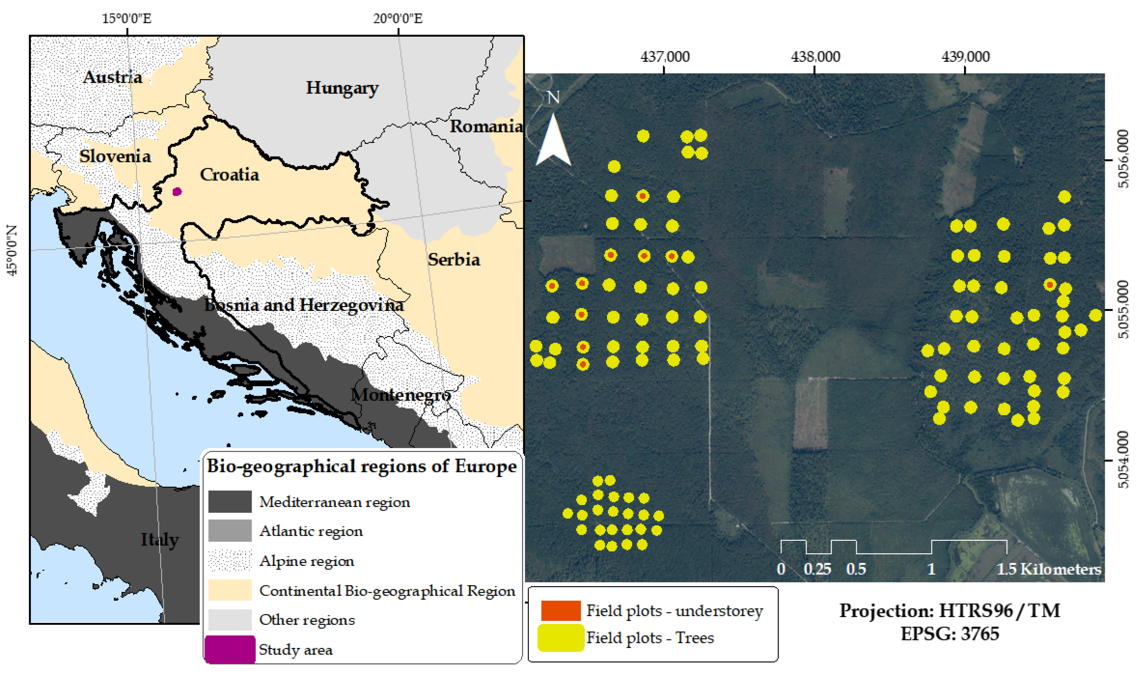
The study area is located in the continental part of Croatia, near Jastrebarsko (35 km southwest of Zagreb), within the Pokupsko Basin lowland forest complex (≈12,000 ha, Figure 2). The forests of the study area consist of even-aged pedunculate oak (Quercus robur L.) stands mixed with other tree species: common hornbeam (Carpinus betulus L.), black alder (Alnus glutinosa (L.) Gaertn.) and narrow-leaved ash (Fraxinus angustifolia Vahl.). Other tree species that sporadically occur are Ulmus laevis Pall., Tilia sp., Populus sp., Acer campestre L., Betula pendula Roth., Pyrus pyraster (L.) Burgsd., etc. Regarding the main vegetation layer (overstorey), this forest commonly has a two-layered structure (dominant and suppressed tree layer) with pedunculate oak in dominant crown-class layer and other tree species in the suppressed crown-class layer. Below the main vegetation layers, the understorey is dominated by two shrub species: hazel (Corylus avellana L.) and common hawthorn (Crataegus monogyna Jacq.), while alder buckthorn (Frangula alnus Mill.) occurs sporadically. Besides shrub species, the young plants of the main tree species are also present in the understorey layer. The relief of the study area is mostly flat (105–118 m a.s.l.). Soils are hydromorphic (hypogley, eugley, pseudogley) on clay parent material. The climate is warm and temperate with the mean annual temperature of 10.6 °C and precipitation of 962 mm y−1 [40].
The pedunculate oak forests of the study area are state owned, and they are actively managed for sustained timber in 140 year-long rotations, ending with two or three regeneration fellings during the last 10 years of the rotation. This management approach provides sustainability in terms of yield, biodiversity and ecosystem stability [41]. It has been applied for all even-aged pedunculate oak forests in Croatia, where they cover an area of 225,000 ha (9% of the total forest area) [42] with 2.43% of mean slope and standard deviation of 2.60%. More detailed information on sustainable management of pedunculate oak forest in Croatia can be found in Ostrogović Sever et al. [40].
2.2. Datasets
2.2.1. Field Data
Field data on overstorey (trees with a diameter at breast height (dbh) above 10 cm; dbh ≥ 10 cm) were collected from a total of 112 circular sample plots during 2017 (yellow circles in Figure 1). The plots were systematically distributed throughout the study area, i.e., within the 30 stands of different age classes and with a total area of 576.32 ha. The radius of plots (8 m, 12 m, 15 m) and systematic distance between the plots (100 m × 100 m, 100 m × 200 m, 200 m × 200 m) were defined in respect to the stand age and size. Positions of plot centres were recorded during the leaf-off conditions (beginning of March 2017) using a GNSS receiver (Stonex S9IIIN, Monza, Italy) connected to the network of GNSS reference stations (Croatian Positioning System—CROPOS Zagreb, Croatia) to achieve high positional accuracy. The average receiver reported the precision of the plots’ positioning was 0.13 m [39]. At each plot, tree species and its location were recorded and diameters at breast height were measured for all trees with dbh ≥ 10 cm. The position of each tree in the plot was recorded by measuring the distance and azimuth from the plot centre to each tree using a Vertex III hypsometer and Haglöf compass, respectively. The tree height was measured for 65% of trees using a Vertex III hypsometer, while heights of the rest of the trees were estimated using the species-specific dbh-height models fitted with Michailloff’s function [43]. More details of this process can be found in Martín-García et al. [44]. In addition to the tree height, the height from the bottom of the tree to the first branch (crown base) was measured for 63.9% of trees. Martín-García et al. [44] hcb equations were applied to those trees without field measurements.

Figure 1.
The location of the study area in Croatia (left) and spatial distribution of sample plots (yellow circles) and sample plots used for validation (yellow circle with an orange dot) within the study area (right).
The second step, returning to the field to take understorey measurements, was conducted in November 2019 (yellow circles with an orange dot in Figure 1). In order to have a reliable understory data source, 10 circular plots with a 15 m radius were selected from a larger set of permanent plots established in 2017, in which understory cover and height were measured. Moreover, within these plots, the understorey consisted only of shrub species and small trees with dbh < 10 cm were not present. Since these measurements were used for understorey evaluation and validation, only plots covered with LiDAR data and with no cuts and slow growth of the vegetation between 2016 (time of LiDAR data acquisition) and 2019 (time of understorey field measurements) were considered for selection. In this way, the selected plots have not undergone modifications in the vegetation structure and composition. In addition, a visual comparison between the field data and LiDAR data was also developed in order to check that there were not discrepancies between the two datasets. Based on this analysis, it was established that two plots, number 47 and 49, show apparent discrepancies as: (i) the shrubs detected from LiDAR data were placed on the edge of the plot; their mass centres were outside the plot (Figure A1, Appendix A), and unfortunately, they were not measured and (ii) LiDAR data show understorey shrubs that do not appear in the field data, respectively. Then, plots 47 and 49 were regarded as “outlier plots” (hereinafter referred to as “outlier plots”). Details of this analysis were included in Appendix A.
The selected plots were located in oak stands of different age ranging from 58- to 93-year-old stands. More precisely, three plots were located in 58-year-old stands, one in a 68-year-old stand, three in 73-year-old stands, and three plots in a 93-year-old stand. Within each plot, the understorey (shrub) species were recorded. To estimate the understorey coverage in the plots (%), for each shrub in the plot two perpendicular lengths (the largest and the smallest) representing the shrub extent were measured using a Vertex III hypsometer as a horizontal distance measurer. Furthermore, for each shrub, the top height was measured using a Vertex III hypsometer.
A summary of the main forest attributes (overstorey) for the plots used to estimate HCB at plot level, as well as for the subsample of 10 plots used for understorey validation (see Section 2.3.3.), is presented in Table 1.

Table 1.
Summary of the main plot-level forest attributes for 112 sample plots used to estimate the height to canopy base at plot level (overstorey) and 10 sample plots used for understorey estimation and validation.
2.2.2. LiDAR Data
The ALS data were acquired under leaf-on conditions within several surveys between 29 June and 25 August 2016 using an Optech ALTM Gemini 167 laser scanner mounted on the Pilatus P6 aircraft. The average flying height was 720 m above ground level with an average flying speed of 51 m∙s−1. The laser pulse repetition frequency was 125 Hz, and the field of view was ±25°. The scanner recorded multiple returns (maximum 4 returns per pulse) resulting in an average point density for the study area of 13.6 points∙m−2. According to the data provider, the horizontal accuracy of the recorded points was 15 cm, and the vertical accuracy was 8.3 cm. The ALS point cloud was classified into ASPRS Standard LiDAR Point Classes [45] using TerraScan software [46].
The ALS data were provided by the Hrvatske Vode Ltd. (Zagreb, Croatia)., whereas the acquisition and pre-processing were conducted by the Institute for Photogrammetry Inc. (Zagreb, Croatia) and Mensuras Ltd. (Maribor, Slovenia).
2.3. Methodology
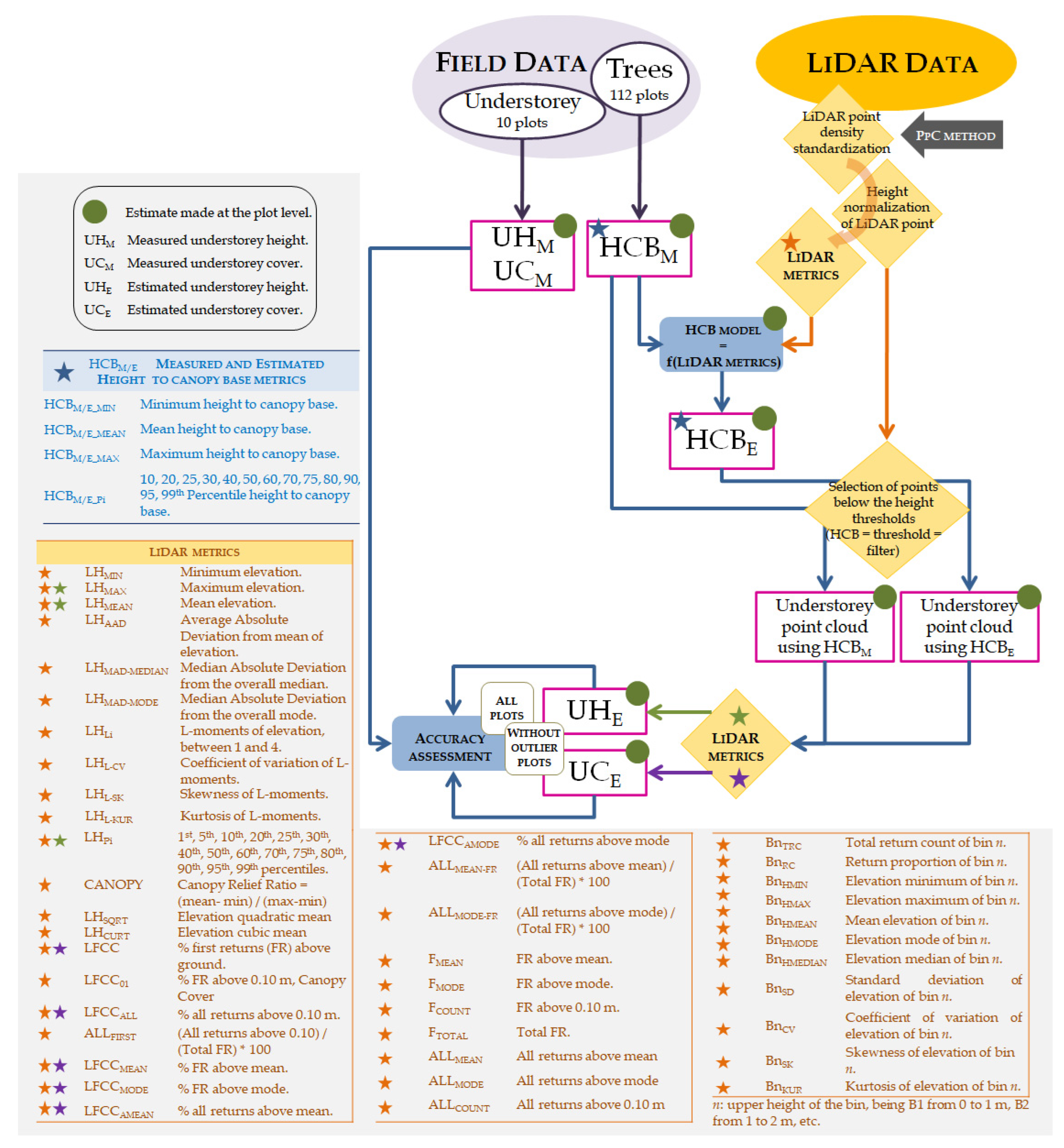
Figure 2 shows an outline of the methodology proposed in this research. This study has been divided into several procedures depending on the data processed and their combination. First, plot metrics were calculated from overstorey field data (Table 2). Then, different distribution statistics of the individual hcb were evaluated to procure a representative value of HCB per plot, hereupon called measured HCB (HCBM). In addition, understorey height and understorey horizontal cover were extracted from understorey field data (UHM and UCM, respectively). Parallel to field-data processing, LiDAR metrics were calculated over the point cloud with standardised density (see Section 2.3.1.). Plot-level HCB models were generated using HCBM and LiDAR metrics as input data (LiDAR metrics with an orange star in Figure 2), and the estimated HCB (HCBE) were obtained. Finally, HCBM and HCBE were applied as filters (the list of HCBs is included in the blue table of Figure 2) to obtain understorey point clouds, and LiDAR metrics were recalculated. The estimated understorey height (UHE) and understorey horizontal cover (UCE) were evaluated over the filtered point clouds (LiDAR metrics with a green and purple star in Figure 2 were used to estimate the UH and UC, respectively). The final step was the validation of these results with the understorey field data.
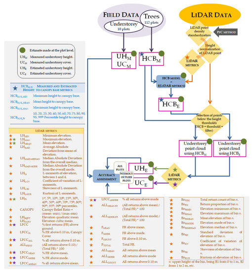
Figure 2.
Workflow of the methodology steps. Green dot—estimates made at plot level; blue star—estimated and measured HCB filters; orange star—LiDAR metrics calculated with the complete point cloud and used in the HCB estimated filters modelling; green star—LiDAR metrics, calculated on the filtered point cloud, used to evaluate UH; purple star: LiDAR metrics, calculated on the filtered point cloud, used to assess the UC.

Table 2.
The goodness of fit parameters and regression coefficients for predicting HCB.
2.3.1. Processing LiDAR Data
Due to the heterogeneity in point density in the LiDAR dataset, point filtering was used to standardise the point density to 6 points·m−2 following Buján et al.’s algorithm [47]. This is particularly relevant in the case of HCB estimation, as a uniform return density of the LiDAR data along the vertical profile is essential [38], since it facilitates that all derived LiDAR metrics have the same representativeness throughout the entire study area.
LiDAR data processing was performed with easyLaz® [48], a proprietary tool based on the FUSION/LDV software [49]. To characterise the vertical distribution of vegetation, the first step was to classify laser pulses into ground and non-ground classes with GroundFilter algorithm implemented in the FUSION software. This method is an adapted version of the Iterative Robust Interpolation algorithm of Kraus and Pfeifer [50]. Classification resulted in 1.09 mean ground points per square meter which were interpolated using the GridSurfaceCreate algorithm implemented in the FUSION software (resolution = 2 m, in this way a mean of 4 points were used to calculate the value of each pixel). Afterwards, the GridSurfaceCreate interpolation function was also used to normalise the LiDAR point cloud. Secondly, a suite of grid metrics was created from the pulse data with the whole range over 10 cm minimum height to remove non-detected soil returns and in 1 m bins up to 20 m in height using the total number of returns (LiDAR metrics with an orange star in Figure 2). The basic concept behind height bins analysis in a vertical profile is to detect in which position the frequency of returns decreases [24,25]. Such a technique is dependent on the “shape” or distribution of return frequencies stratified by height [5]. The goal of this procedure is to search for a relationship between different statistics of height and density of LiDAR pulses focused on a definite interval and the height to the canopy base.
2.3.2. Estimates of HCB Models
Firstly, it needs to be clarified that in this study, as in previous studies [5,38], the understorey was defined as suppressed trees and shrubs growing beneath an overstorey canopy. The hypothesis of this study is the lower height of that overstorey canopy may be set from HCB. That said, several HCB were calculated per plot (HCBM) from the field data (112 plots—yellow circles in Figure 1). The list of HCBs is included in the blue table of Figure 2. These HCBM will be hereupon called “filters”, as they will be used as such for the LiDAR point cloud. Then, potential (Equation (1)) and exponential (Equation (2)) models were tested to find the optimal empirical relationships between the different HCBM and LiDAR metrics (LiDAR metrics with an orange star in Figure 2). Parameters ai are to be estimated and xi are LiDAR metrics.
We used the linearised form of both equations to fit the models with ordinary least squares with lm function from stats package v.4.1.0 [51] in R software v.3.6.2 [52]. The inherent systematic bias of the prediction when undoing the linearisation was corrected following Sprugel [53]. Variable selection was performed with the function regsubsets of the package leaps v.3.1 in R software v.3.6.2 [52].
Models were selected and inspected graphically, and evaluated numerically through the root mean squared error (RMSE), both absolute and relative (in meters and percentage, respectively); mean error (bias) in percentage and its p value to assess whether it is significantly different from zero; the coefficient of determination (R2) of observed versus the predicted percentage; and the model efficiency (EF) percentage, which is commonly used to assess the model performance (values nearer to one indicate a model with more predictive skill). Finally, to avoid overfitting, the vif function of the package car v.3.0-10 [54] was applied to select the most parsimonious model.
2.3.3. Understorey Analysis and Assessment
The process of understorey analysis consisted of three steps. First, the original point cloud relating to the 10 plots with understorey field data was filtered using both the measured and the estimated HCB as upper thresholds. Each HCB (measured or estimated) produced different filters and generated different understorey point clouds. Secondly, several metrics were calculated on the filtered point cloud with easyLaz® for each understorey point cloud filtering (the LiDAR metrics with a green and purple star in Figure 2). We established a lower threshold of 10 cm for point cloud returns to remove noise, herbaceous and non-detected ground points. Finally, the estimation of UH was calculated through the mean height and the height percentiles collated in the orange table in Figure 2 (metrics with a green stars) of the filtered point cloud. To estimate UC, LFCC, LFCCALL, LFCCMEAN, LFCCAMEAN, LFCCMODE and LFCCAMODE metrics were evaluated (see acronyms in the orange table in Figure 2—metrics with a purple star). Martinuzzi et al. [29] found the use of two understorey airborne LiDAR metrics along with a common slope-aspect transformation variable that could accurately estimate the presence of shrub cover (accuracy: 83%). The two understorey LiDAR metrics utilised in their study were the percentage of ground points and percentage of points between 1 and 2.5 m compared to all plot points. Additionally, most of the studies consulted used variables related to the number of points to estimate UC [11,24,29,30]. For this reason, in our study the variables related to percentage of points were used to estimate UC.
To assess which combination of metrics and HCB filters get the best UH and UC predictions, we validated the results with the field data by calculating the RMSE (absolute and relative) and bias of the differences between observed and predicted values (UHM—UCM vs. UHE—UCE). In addition, a sensitivity analysis based on the relative RMSE was performed in order to evaluate the influence of several factors on the UH and UC estimate. For this purpose, the plot.design function on graphics package v 3.2.1 [53] was used. This function plots the magnitude of the effect of each factor on the dependent variables, in this case represented by the relative RMSE. This plot is calculated by considering the levels of the different factors independently: the factors are plotted on the x axis, while the levels for each of these factors are plotted as a vertical line. The longer this vertical line, the greater the influence of the factor on the quality of UH and UC estimates. In addition, the relative RMSE average is represented by a horizontal line [47]. The following factors and their levels were analysed: HCB filters (levels: HCB included in blue table of Figure 2), plots used (levels: all plots and sample without outlier plots), type of HCB (levels: measured and estimated) and metrics (levels: LiDAR metrics with a green and purple star in Figure 2).
3. Results and Discussion
3.1. Estimates of HCB Filters
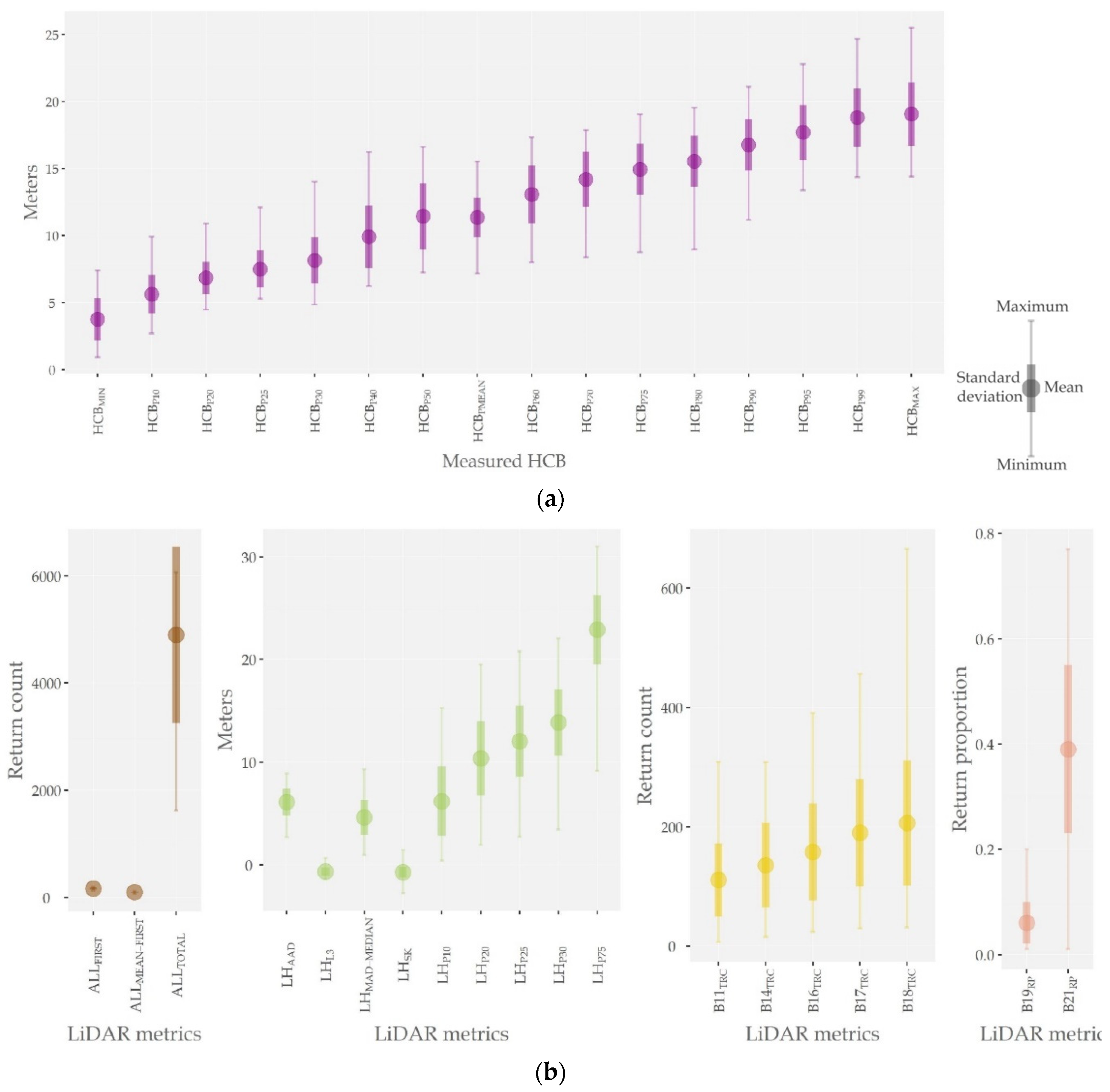
Figure 3 displays the statistical summary (mean, minimum, maximum and standard deviation) for the dependent (HCBM) (Figure 3a) and independent variables (LiDAR metrics) present in the models (Figure 3b). LiDAR metrics can be grouped into three blocks: variables that describe the number of returns (ALLTOTAL, ALLFIRST, ALLMEAN-FIRST), vertical profile descriptive variables of the total vegetation (LHPx) and descriptive variables by bins (Bix). The HCBM filters with the highest variability are HCBP50, HCBMAX and HCBP40, while ALLTOTAL, LHP20 and B18TRC are the independent variables with the highest variability. On the other hand, the dependent and independent variables with the lowest variability are HCBP20 and B19RP, respectively.

Figure 3.
Statistical summary (mean, minimum, maximum and standard deviation) of (a) dependent variables (HCBM) and (b) predictor variables (parameter) of the HCB models (see acronyms in Figure 2). Quantitative results were included in Table A1 (Appendix B).
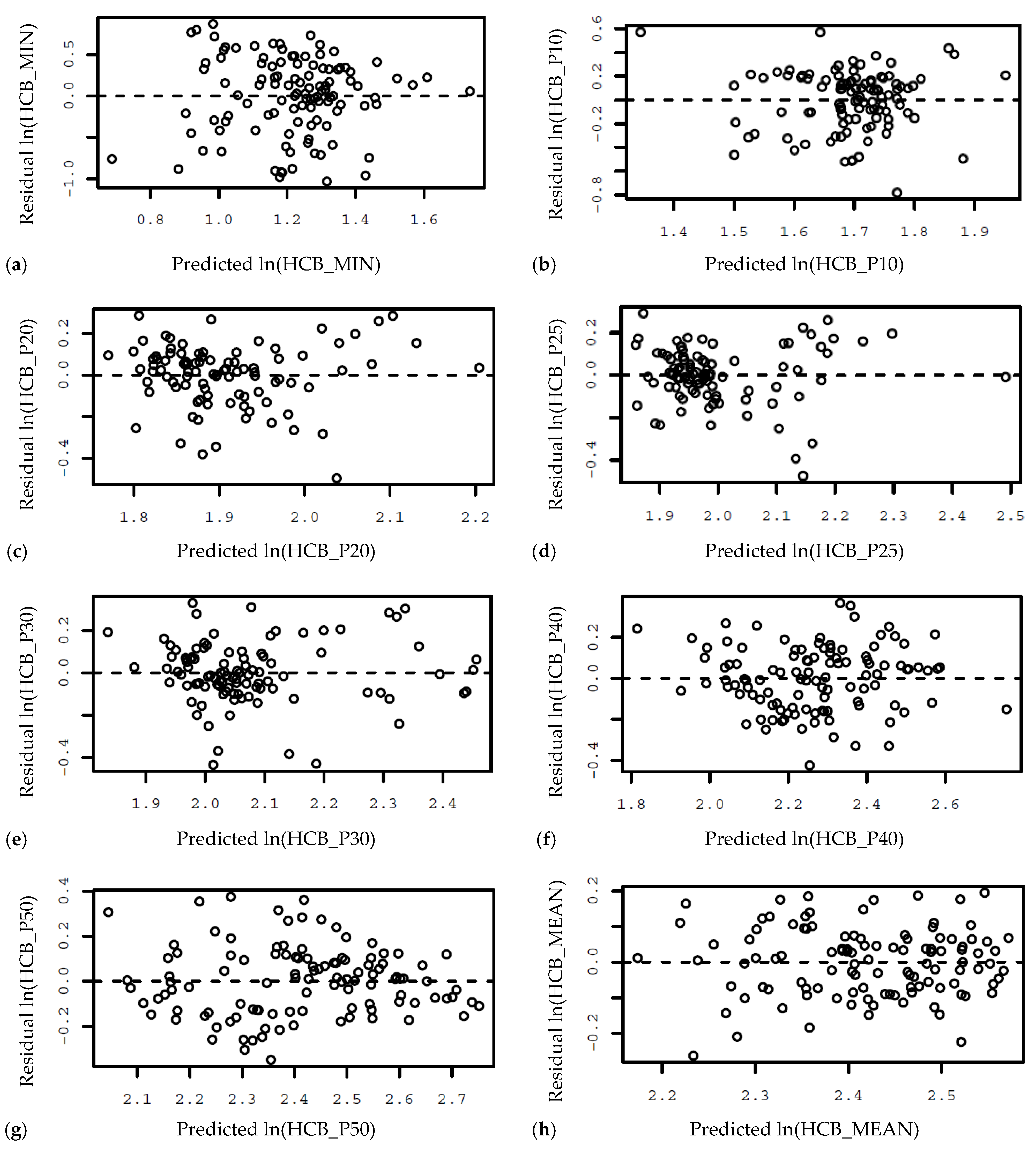
Table 2 presents HCB models of the different filters using LiDAR metrics. Residual versus predicted plots are attached in Figure A4, Appendix B. Relative RMSE values range between 7.73% for HCBMAX and 40.31% for HCBMIN; the absolute RMSE is lower than 1.70 m in all cases. HCB metrics using percentiles equal or above the mean (HCBMEAN, HCBP60, HCBP70, HCBP75, HCBP80, HCBP90, HCBP95, HCBP99 and HCBMAX) are predicted more accurately by the LiDAR metrics than the other HCB models. The efficiency (EF) varies between 7.01% (HCBMIN model) and 60.61% (HCBMAX model). None of the models showed significant bias (p-value > 0.05). Finally, the results show a slight overestimation in 14 of the HCB models. Within each plot, several species and different stages of development coexist as it is a mixed, mostly two-layered forest, making the measurement of the HCB per plot imprecise. A mean measurement of the individual HCB values is not sufficient to capture the existing variability.
The HCBP70 and HCBP75 models have selected the same predictor variables (ALLMEAN-FIRST, B14TRC and B16TRC). The same situation is found in the HCBP80, HCBP90 and HCBP95 models, whose predictor variables are also common (LHP75, B14TRC and B16TRC). This phenomenon can be explained by the summary statistics proximity collected in Figure 3 for these HCB filters. On the other hand, though at least one metric describing the entire vertical profile of the vegetation (LHi) enters in 80% of models, the bin metric (e.g., B16TRC and B14TRC) are the most explanatory variables. The combination of percentile and the fraction of points in several LiDAR bin metrics has been used to fit regression models in previous studies [38].
The HCB estimate through LiDAR metrics have presented a wide range of correlation coefficients (R2) between 31.12% for the HCBMIN model and 78.35% for the HCBMAX model. Our results are similar to the research conducted by other authors. Maguya et al. [55] obtained high RMSE and low consistent RMSEcv with HCB LiDAR models based on traditional percentile due to the high degree of correlation among the variables. Their best result was 65% of R2 with 1.62 m RMSE. Luo et al. [56] evaluated HCB models based on different tree-height groups (less than 15 m; 15 to 25 m; 25 to 35 m and >35 m) obtaining correlations between 52% and 86%, which improved as the height of the group of trees studied increased. These results improve those obtained by Stefanidou et al. [38], who found a correlation of 15%, applying voxel-based estimation, and 75% applying a linear regression model.
3.2. Understorey Evaluation
3.2.1. Understorey Height Evaluation
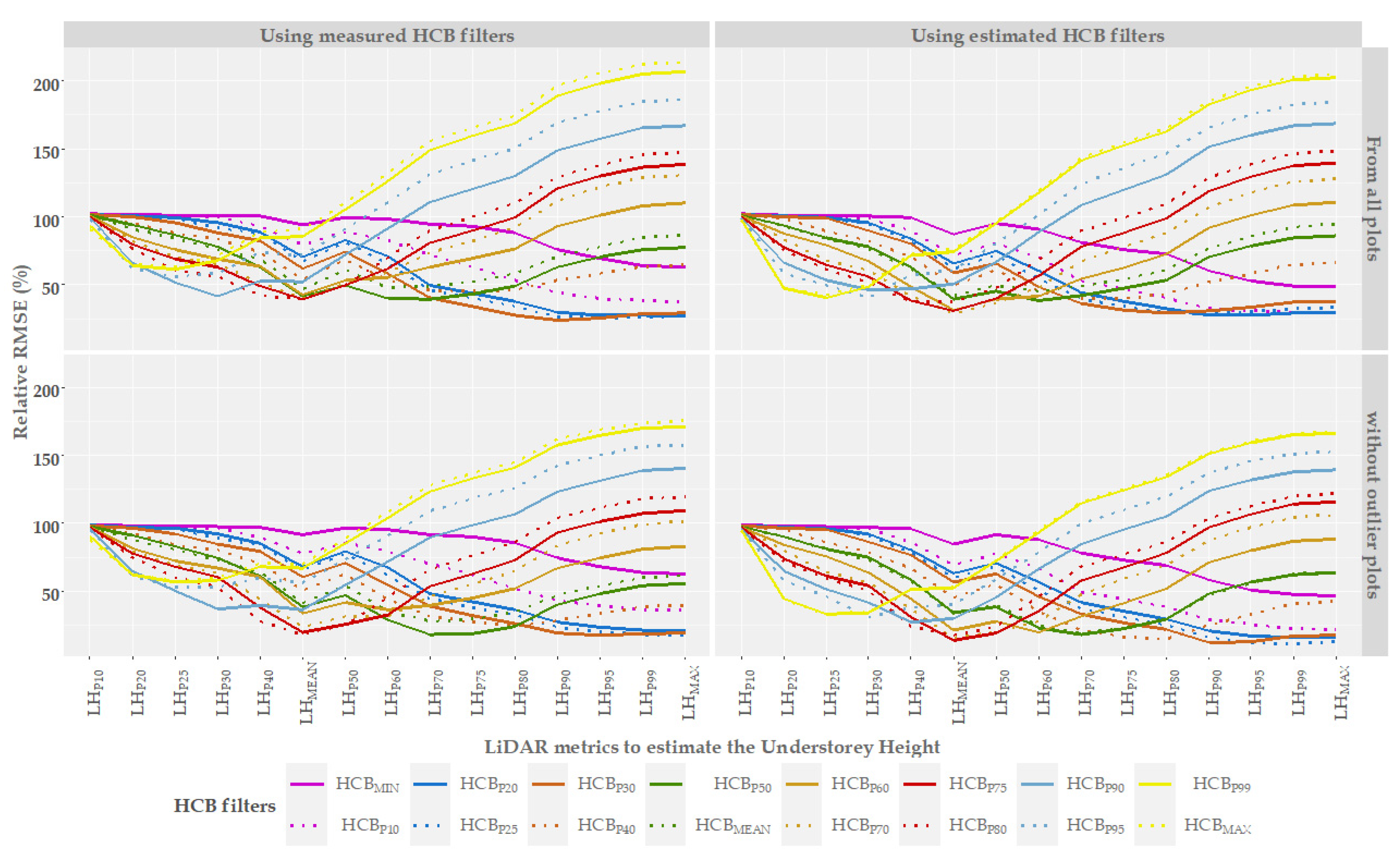
To evaluate the UH, 15 LiDAR metrics per filtered point cloud were analysed. Figure 4 shows the performance of different LiDAR metrics with respect to HCB filters, both measured (first column in Figure 4) and estimated (last column), to estimate the UH using all plots (first row in Figure 4) and a sample without outlier plots (last row) (without taking account plots 47 and 49).
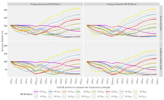
Figure 4.
Results of estimated UH: relative RMSE (%) (y axis) for HCB models (filters applied) and for each metric appraised (x axis) using all plots and a sample without outlier plots (rows in facet grid figure) and measured/estimated HCB models (columns in facet grid figure). Note: The complete set of metrics in UH evaluation and their errors are included in Supplementary Materials—Table S1.
In general, for HCBM-i and HCBE-i filters, the metrics appraised present two types of behaviour: (i) if HCB filters ϵ (HCBMIN, HCBP10, HCBP20, HCBP25, HCBP30), Figure 4 shows an inverse relationship between relative RMSE and LiDAR metrics, i.e., the relative RMSE decreases as the percentile of LiDAR metric increases and (ii) if HCB filters ϵ (HCB40, HCBP50, HCBMEAN, HCBP60, HCBP70, HCBP75, HCBP80, HCBP90, HCBP95, HCBP99, HCBMAX), Figure 4 shows an inverse and direct relationship between relative RMSE and LiDAR metrics, where LHMEAN metric is the inflection point. Although the plots have similar ecological characteristics, the overlap of tree and shrub canopies varies among plots, which visibly influences the estimates obtained. For this reason, if we apply filters of the higher percentiles or the maximum value of HCB, submerged crowns could be kept, and the understorey measurements overestimated. On the contrary, when filters of the lower percentiles or the minimum value of HCB are applied, returns belonging to the larger bushes may be eliminated and underestimate the measurements, excluding returns that remain between the filter made and the actual crown base height. For the metric 10th percentile, all the HCB filters have a relative RMSE close to 100%. So, the metric LHP10 is the least sensitive to the establishment of height thresholds. From this metric to the metric LHP60 (along the x-axis in Figure 4), their sensitivity in the face of HCB filter variations is very similar. However, it increases considerably until it reaches its maximum value using LHMAX. This metric is the most sensitive to variations in the HCB filter. In the last case, the use of the HCBP25 filter shows a relative RMSE that ranges from 25% to 75% (using estimated HCB filters—without outlier plots and using estimated HCB filters—all plots, respectively), while the HCBMAX filter shows a relative RMSE that varies between 160% (using estimated HCB filters—without outlier plots) and 225% (using measured HCB filters—all plots).
Although the trends observed above are independent of measured/estimated HCB filters and all plots/without outlier plots, Figure 4 shows the relative RMSE decreases in all UH evaluations using a sample without outlier plots; however, the same RMSE is obtained using measured/estimated HCB filters.
Estimates of the mean understorey height were calculated from estimated and measured HCB filters using all plots and a sample without outlier plots and were compared to field measurements. The best results of this analysis were included in Table 3. Considering these results, LiDAR metrics—specifically LHP75, LHP80 and LHP95—utilising the point cloud filtered with HCBP25 were generally effective for quantifying the mean understorey height. Interestingly, RMSE decreased more using the estimated filters than the measured filter without outliers. In a specific way, the results using the estimated HCBP25 filter and the LHP95 LiDAR metric show the highest correlation (R2 = 0.80; p-value = 0.0179) and the lowest RMSE (RMSE = 0.88 m). These results improve the estimates obtained in previous research, setting aside the differences between those studies. For example, Sumnall et al. [5] found a high correlation between filtered point clouds and field measurements for estimating the maximum understorey height (R2 = 0.75; RMSE = 2.90 m), thereby improving the results reported by Goodwin et al. [25] or Su and Bork [33], where no relationship between LiDAR metrics and field data for calculating the maximum UH was found. The point density is one of the main differences between these studies (Sumnall et al. [5], 10 pulses/m2; Goodwin et al. [25], 1 point/m2; Su and Bork [33], 0.54 points/m2). However, Hill and Broughton [6] linked these results with the fact that the dominant trees form a dense and closed canopy, preventing the laser pulses from penetrating the overstorey canopy.

Table 3.
Understorey height: Summary error statistics produced by assessing field measurements and LiDAR metrics.
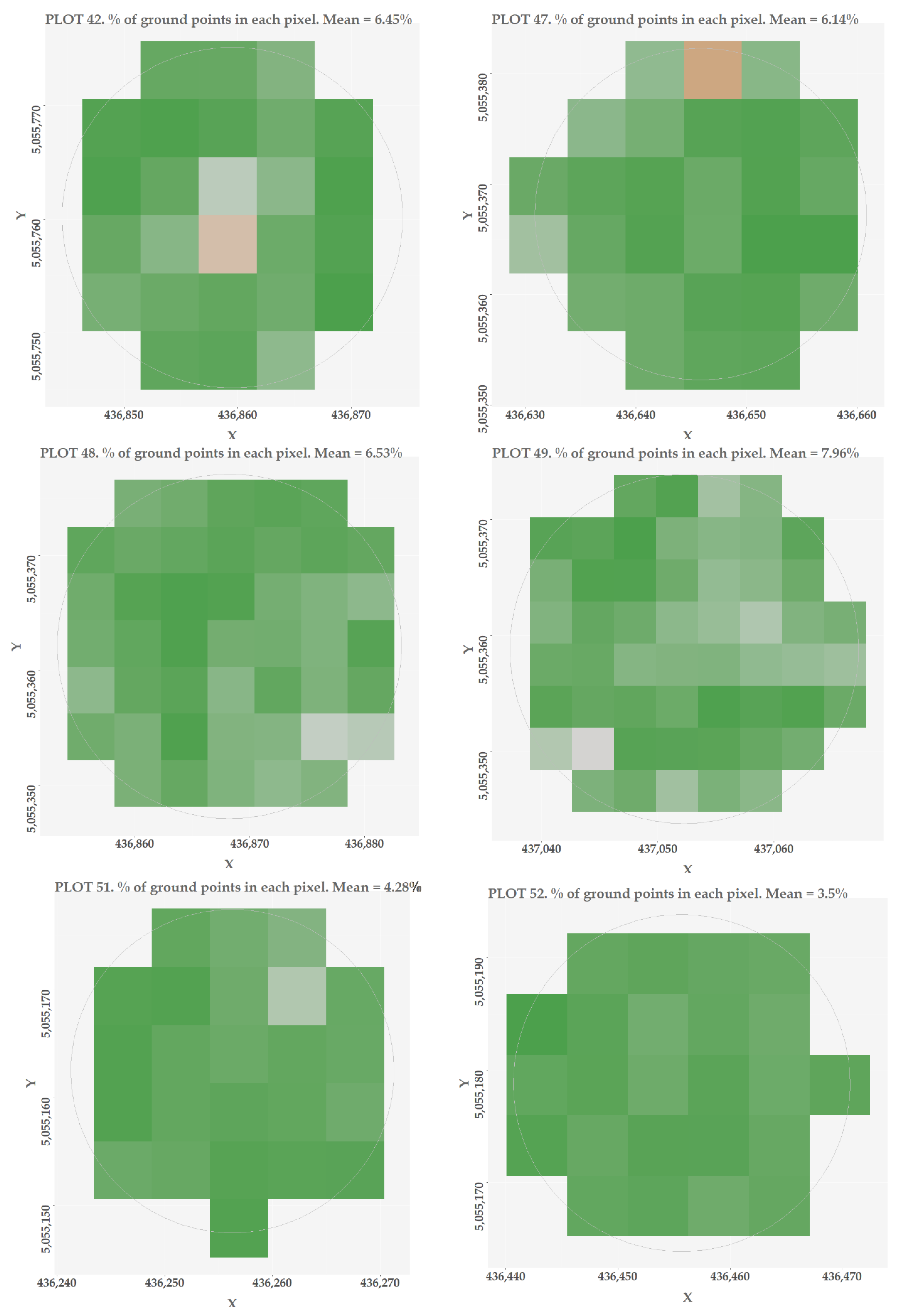
Taking into account the results of filter-metric combinations included in Supplementary Materials—Table S1 at plot-level, plot 49 had higher overestimation errors (mean error = −3.15 m: HCBE-P25-LHP95 error = −4.84 m; HCBM-P25-LHP80 error = −1.46 m). The causes of these discrepancies have already been described in Section 2.2.1. These errors explain why the elimination of the outlier plots reduced the RMSE in both measured and estimated HCB filters, and why the RMSE decreased more in the estimated filter than in the measured filter. In addition, the major underestimation errors occurred in plot 58 (mean error = 2.53 m: HCBE-P25-LHP75 error = 2.86 m; HCBE-P25-LHP95 error = 1.12 m; HCBM-P25-LHP75 error = 3.23 m; HCBM-P25-LHP80 error = 2.89 m) and plot 134 (mean error = 2.67 m: HCBE-P25-LHP75 error = 3.34 m; HCBE-P25-LHP95 error = 1.64 m; HCBM-P25-LHP75 error = 3.07 m; HCBM-P25-LHP80 error = 2.65 m). This finding is consistent with the reported tendency for shrublands by Su and Bork [33]. These errors were attributed to LiDAR points which usually intersect the sides of the shrub canopy, but not the shrub top. In addition, previous studies have shown the inverse relationship between the canopy cover and the accuracy of understorey estimates [25,30,33]. This is principally related to the fact that the number of LiDAR returns from the lower strata is reduced as the canopy permeability decreases [5]. Although the impact of the canopy cover on the understorey estimates has not been analysed in our study, it is noteworthy that the previous plots (plots 58 and 134) have the highest percentages of ground points, i.e., the highest permeability (7.62% and 8.97%, respectively) (Figure A3, Appendix A). These values show that a higher point density is required for the analysis of sub-canopy features. Theoretically, if the permeability is 10%, then it is necessary for a density of 10 pts/m2 to reach 1 ground/sub-canopy point per m2.
Goodwin et al. [25] showed the relationship between the ability to estimate understorey structure and the percentage of first returns (FR) recorded from the understorey layer when the percentage of FR is greater than 50%. In our study, 3.6% (mean value) of all FR are placed in the understorey layer and this percentage is 3.89% and 7.47% in the plots 58 and 134, respectively. Despite the fact that these plots also have the highest percentages of FP in the understorey layer, those values are less than 50% observed by Goodwin et al. [25] and that relationship was not found in our study. However, these circumstances have been relegated to second place because the field mean height records (7.58 and 8.71 m, respectively) are greater than the upper height thresholds using HCBP25 filter (6.99 and 7.67 m, respectively), which really might explain the underestimation errors. In the same way, Stefanidou et al. [38] found an underestimation of the HCB, with the consequent underestimation of the understorey, since this vegetation layer creates a continuous vertical point distribution. In either case, as it is a mixed forest, these errors are compensated throughout the plot by the inherent variability of these formations. In addition, a part of the error in our measurements is probably due to the time lapse between the LiDAR measurements (2016) and the understorey field-data collection (2019). However, it can be assumed that dimensions (height, diameters) of understorey (shrubs) were not changed significantly during this period. First of all, a dense and closed canopy layer that prevents greater penetration of light to the understorey is present in all observed plots. Furthermore, in the period 2016–2019, there were no cuts of large trees from the overstorey layer within the observed plots that could provide more light for the understorey and greater stimulus to its growth.
On the other hand, Andersen et al. [7] reported a correlation coefficient of 53 and 9% under Douglas fir stands between 95 and 65 years old, which were the worst results in the youngest stands. In this work, understorey was the vegetation between 1.8 m and the base of the overstorey. Latifi et al. [8] found 80% R2 in shrub, considering this layer as the understorey without herb or moss. Venier et al. [30] found an explained variance of 87%, a cross-validation error of 15.6% using a voxel-based model, and explained 74.4% of the variance with 12.9% cross-validation error employing a Random Forest model. In this research, the understorey layer was all vegetation under 4 m. These results reflect the variability of criteria regarding which vegetation to include as part of the understorey. Although the differences seen are due to the different floristic composition of each studied stand, the state of development and topography, among other aspects, it would be necessary to standardise the nomenclature to be applied, creating more than one layer of sub-canopy, shrubby understorey vegetation and herbaceous understorey. The defined layers could be studied independently of the existence of all of them in the same study area.
3.2.2. Understorey Cover Evaluation
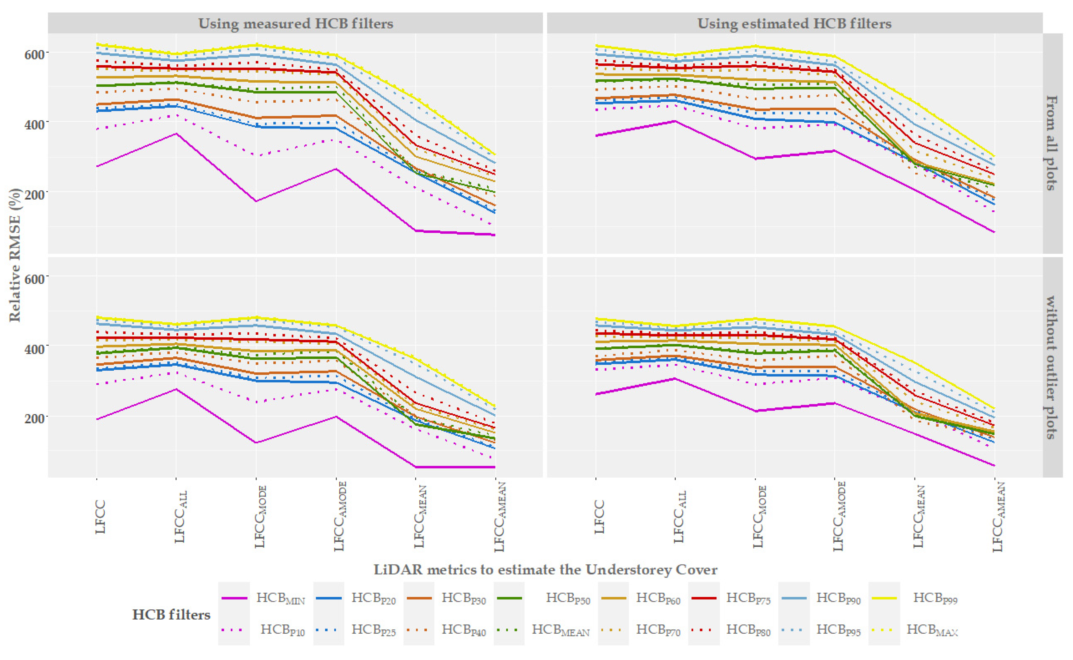
Six LiDAR metrics per filtered point cloud were studied in the UC evaluation. Figure 5 shows the evolution of the RMSE in the six metrics used to evaluate UC according to the HCB filters used. Organised in the same order as Figure 4, measured HCB filters are in the first column, estimated HCB filters are in the second, and sample without outlier plots (plots 47 and 49) are in the last row.

Figure 5.
Results of estimated UC: relative RMSE (%) (y axis) for HCB models (filters applied) and for each metric appraised (x axis) using all plots and a sample without outlier plots (rows in facet grid figure) and measured/estimated HCB models (columns in facet grid figure). The complete set of metrics in UC evaluation and their errors are included in Supplementary Materials—Table S2.
In general, Figure 5 shows a relative RMSE decrease for the LFCCMEAN and LFCCAMEAN metrics in all applied filters and, although in a lower degree, also in LFCCMODE for the HCBP10 and HCBMIN filters, and LFCC for the HCBMIN filter. For the rest of the HCB filters (HCBP20, HCBP25, HCBP30, HCB40, HCBP50, HCBMEAN, HCBP60, HCBP70, HCBP75, HCBP80, HCBP90, HCBP95, HCBP99, HCBMAX) the relative RMSE values remained almost constant in the LFCC, LFCCALL, LFCCMODE and LFCCAMODE metrics. In all cases, the RMSE was greater in the filters that represented a higher HCB, although in the LFCCMEAN metric in HCBM filters ϵ (HCBP50, HCBMEAN), the RMSE decreased in values lower than the result obtained for the HCBP20 filter. For the HCBE filters ϵ (HCBP50, HCBMEAN, HCBP60), the RMSE decreased similarly to the result obtained for HCBP10. The elimination of the outliers (plots 47 and 49) reduced the RMSE in all filters. RMSE decreased more in the estimated filter than in the measured filter without outliers.
There are two factors that trigger the relative RMSE to values between 400 and 650. The first is to use the HCB filters that reflect higher heights and the second is to apply metrics that consider a higher percentage of pulses when evaluating the understorey. In these cases, the lower branches of higher trees as well as submerged trees are included in UC, overestimating the actual value measured in the field. The use of lower height filters, together with statistics that count pulses from a lower height, LFCCMEAN and LFCCAMEAN, mitigates this overestimation. As in the estimation of UH, this is due to the different overlap of tree and shrub canopies from plot to plot, despite the study area having similar ecological characteristics.
All metrics present constant sensitivity throughout the different applied filters, except the LFCCMODE metric, which presents a greater variation depending on the applied filter. Relative RMSE increases slightly in LFCCMODE for the filters corresponding to the higher percentiles (HCBP90, HCBP95, HCBP99, HCBMAX); it remains constant for the filters (HCBP60, HCBP70, HCBP75, HCBP80) and decreases for those of lower height (HCBMIN, HCBP10, HCBP20, HCBP25, HCBP30, HCBP40, HCBP50, HCBMEAN). Relative RMSE in the LFCC metric presents sensitivity in the HCBMIN filter, which highly decreased. On the other hand, the LFCCAMEAN metric is the one that offers more stable and lower values for all applied filters.
There are no significant differences between measured and estimated filters, except for the HCBMIN and, to a lesser extent, for HCBP10 filters, where the relative RMSE decreases drastically when considering the measured instead of the estimated filters. Relative RMSE decreases considerably when removing outliers in both measured and estimated filters.
Table 3 and Table 4 show the best results of the mean UC derivatives of estimated and measured HCB filters estimates using all plots and a sample without outlier plots (without plots 47 and 49) and compared to field measurements.

Table 4.
Understorey cover: summary error statistics produced by assessing field measurements and LiDAR metrics.
The values of LFCCAMEAN and LFCCMEAN metrics obtained from the point clouds filtered with estimated and measured HCBP10 and measured HCBMIN filters showed the best results in the UC calculation. Contrary to what happens in the case of the UH, the RMSE decreases more when the plots with anomalous values are eliminated in the measured filters, instead of estimated filters.
Specifically, LFCCAMEAN obtained from the point cloud filtered with HCBP10 have the highest correlation (R2 = 0.84; p-value = 0.0022) using all the plots in the calculation of UC. The LFCCMEAN metric estimated from the filtered cloud with HCBMIN without anomalous plots has obtained the highest precision (53.73% relative RMSE), but this analysis is biased (p-value = 0.0548). Since no analysis excels in all the parameters studied, we have considered the combination of HCBP10 filter and LFCCAMEAN metric with the elimination of plots with outliers as the best result, presenting a high correlation (R2 = 0.81; p-value = 0.0144), although the relative RMSE is high (107.55%). Similar results were obtained by Goodwin et al. [25], with R2 values between 0.68 and 0.87 in a multi-use forested area where Western hemlock (Tsuga heterophylla) is the dominant species; by Skowroski et al. [57], with R2 values of 0.74 in Pitch Pine lowlands and 0.59 in mixed hardwoods; Wing et al. [24], with R2 values of 0.70–0.80 in ponderosa pine (Pinus ponderosa Dougl.), stands accompanied by other secondary species, and Sumnall et al. [5] found R2 values of 0.82 (unfiltered data) and to 0.83 (filtered data) at plot level in multi-layered Loblolly pine (Pinus taeda L.) forest.
Considering the results of filter–metric combinations included in Supplementary Materials—Table S2 at plot level, the major overestimation errors in cover percentage occurred in the plot 47 (Mean error = −18.92: HCBE-P10-LFCCAMEAN error = −14.67; HCBM-MIN-LFCCMEAN error = −23.17). As in UH calculation, outlier-plots elimination reduces the RMSE in estimated HCB filters and, to a lesser extent, in measured HCB filters. In addition, the plot 134 (Mean error = −16.46: HCBE-P10-LFCCAMEAN error = −18.35; HCBM-P10-LFCCAMEAN error = −15.96; HCBM-MIN-LFCCMEAN error = −13.19) also shows a very high overestimation.
Results accuracy is conditioned by two factors: (1) the vertical distribution of vegetation in multi-layered overstorey, and (2) the penetrability of the LiDAR pulses. Previous research shows that plots where understorey canopy layers and dominant layers intermix were more prone to errors [5,24] and higher overstorey canopy densities typically occlude laser [5,6,58], which makes it difficult to discriminate 3D point cloud information into recognisable structures within a forest context [5,59]. In our study area, the combination of these two factors has negatively influenced the result.
The decrease in LiDAR pulses in the understorey due to canopy occlusion is more evident at lower pulse densities, such as in Su and Bork [33], with densities of 0.54 points m−2, although it also negatively affects studies with higher LiDAR densities, as in Wing et al. 2012 with 5.4 points m−2. However, Venier et al. [30] found larger errors in the highest understorey stratum (2.5–3.5 m) than in the lowest (0.5–1.5 m) with 11.69 points m−2, suggesting that there was no reduction in the estimations associated with potential occlusion [30]. This is consistent with our work, since no relationship was found between a lower point density and an increase in estimates error with mean understorey pulse density of 1.28 points m−2 (15.59% of total returns). Nevertheless, LiDAR acquisition during overstorey leaf-off conditions and understorey leaf-on conditions to increase understorey LiDAR point densities would be recommended, but this is difficult in areas with dense overstorey conditions that would also increase acquisition costs [24].
The relationship among understorey species, height and size for each plot has been analysed (Figure A2, Appendix A). Although plot 134 is the one with the highest understorey height (8.71 m), there is no clear relationship between understorey height and understorey cover estimate. Likewise, no relationship between field coverage and the errors obtained has been seen. In contrast, Sumnall et al. [5] actually found that uncertainty increased as horizontal cover and height increased. In addition, no relationship was observed between the understorey species and the errors observed. This is consistent with the research by Venier et al. [30] that did not observe any influence of the vegetation on the understorey cover predictions, which allows the understorey to be predicted only from LiDAR, reducing field work and its cost.
Plot size also influences the relationship between measurement and estimation from LiDAR variables. Goodwin et al. [25] (R2 0.87 at plot level and 0.68 at subplot level) found that this relationship became weaker as the size of the plots decreased. Understanding the effects of increasing plot size on model variability would help to determine the most efficient sampling design [24]. Although all our plots were the same size, it seems reasonable to think that by applying the models to larger study areas, the mean errors would be compensated and therefore predictions would be improved.
There is a great deal of research studying the understorey characteristics below a given height (Skowronski et al. [57] between 1 and 4 m height; Gopalakrishnan et al. [60] from ground less than 3 m; Venier et al. [30] from 50 cm to 4 m). This type of methodology is conditioned to the forest type, and its application is less reliable in larger areas. The methodology proposed here has the advantage of adapting to the peculiarities of complex forest formations and could be extended to larger extensions of the territory. Similar studies have been used successfully, e.g., Riaño et al. [59] performed cluster analysis to determine crown base height, and thus, tree and understorey heights for estimating fuel loads.
3.3. Effects of Factors on the Quality of UHE and UCE
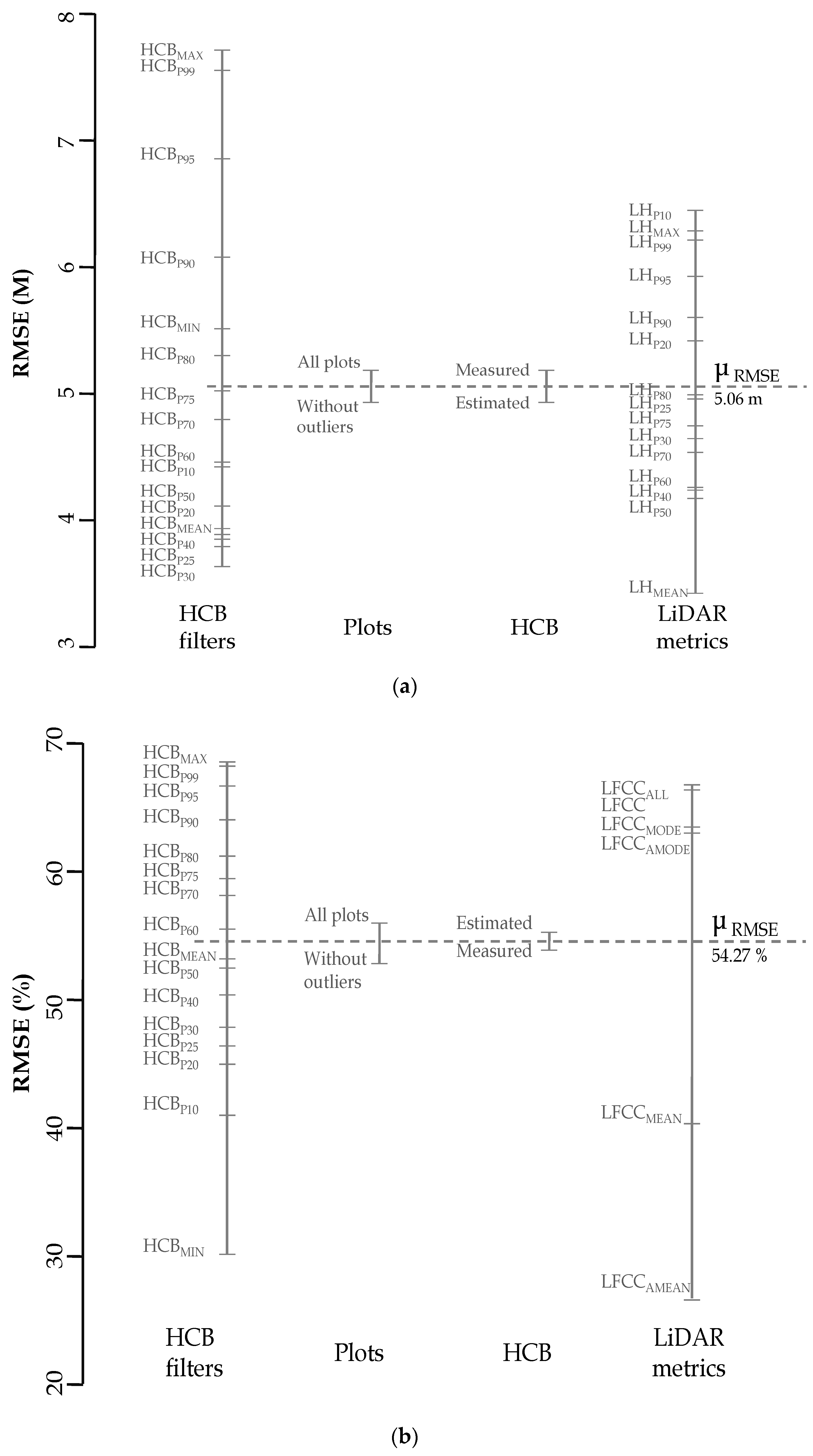
Figure 6 shows the results of the sensitivity analysis produced by the plot.design function. The factors are plotted on the x axis, while the levels of each of these factors are plotted on a vertical line. In addition, the length of the vertical line indicates the influence of factors in relation to RMSE, and the mean value of this measure is represented by the horizontal dashed line. According to this information, the HCB filter, which was used as the upper height threshold to select the understorey LiDAR points, is the most important factor affecting the estimates of UH (Figure 6a), while this factor and the LiDAR metric are the most important factors affecting the estimates of UC (Figure 6b). Despite the importance of the HCB filter for the estimates of UH and UC, the distributions of HCB-filter levels along their vertical lines are different. While in the second case (UC—Figure 6b) the LiDAR metrics are almost as important as the type of filter when determining the precision of the estimates, LFCCAMEAN and LFCCMEAN are clearly better than the rest of the metrics when estimating UC. The type of filter, measured vs. estimated, is less important than in the UH case study, although it is noteworthy that in this case the measured filters offer better results.
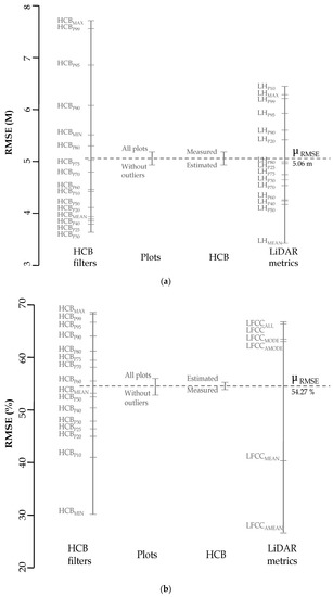
Figure 6.
Results of the sensitivity analysis for: (a) UH with a mean RMSE of 5.06 m (RMSEr: 77.27%) and (b) UC with a mean RMSE of 54.27 percentage cover (RMSEr: 373.73%).
On the other hand, the type of HCB (estimated or measured) and plots used (all plots or without outlier plots) have much less influence on the estimates of UH and UC than the other factors considered. In both cases (UH and UC estimates), the use of a sample without outlier plots slightly improves the results of the understorey estimates. These results also show how the use of estimated HCB filters, against the use of measured HCB, does not significantly influence the accuracy of the estimates. Even in the case of UH estimates, the results using estimated HCB filters are better, which was evidenced in the previous section (Figure 4). Considering these results, the use of upper height thresholds using estimated HCB filters would facilitate the applicability of this method and also allow field works to be dispensed, with the consequent reduction in costs, in regions with similar characteristics.
Considering the effect of the HCB filter on the mean UH estimates, the influence of this factor on the estimates of the understorey maximum height could be much higher, especially when the HCB filter is smaller than the maximum UH, which may result in an underestimation of UH. It is important to note, however, that this is just one possible interpretation of the results, which might be affected by other issues, such as the design of multi-return LiDAR systems (“blind spot”), the point density, the canopy penetrability, the overlapping vertical layers, the vertical continuity of vegetation, among others [5,24]. Moreover, despite the importance of the upper height threshold, to our knowledge, this factor has not been analysed in previous studies. On the other hand, the effect of other factors, such as the terrain slope, on the estimates of UH and UC has been analysed in previous studies, although a relationship between the slope and the understorey estimates has not been found [26]. In our study, the slope has not been analysed; however, our results show no evidence of the influence of this factor, since the field plots show a large enough number of ground points to accurately model the bare ground (Figure A3, Appendix A).
4. Conclusions
In this study, plot-level UC and UH were estimated for an even-age mixed deciduous forest based on airborne LiDAR data. The novelty of our approach is to use HCB models, derived from field measurements and LiDAR metrics, as point cloud filters to remove canopy layer noise to obtain more accurate UC and UH estimations. Since several species and different stages of development coexist, a mean measurement of the individual HCB values is not sufficient to capture the existing variability. The developed HCB models have the advantage of adjusting throughout the forest horizontal area depending on its structure and could be extrapolated to higher study areas. HCB models in the larger percentiles have shown fairly robust behaviour, both in terms of goodness-of-fit parameters and consistency in the selected independent variables, since those HCB models whose values were close (e.g., HCBP80, HCBP90, and HCBP95) share the same independent variables and their accuracy improved with the filter height.
The two sets of filters, measured and estimated HCB, have given similar results, proving that both methods are comparable. In view of the performance of both validations, we can state that it is possible to estimate the understorey with LiDAR data, obtaining similar precisions in the UC and UH estimations. This represents cost savings when obtaining information on the structure of the understorey and the possibility of generalising the output for a whole stand on a wall-to-wall basis. In addition, the fact that the UH obtains better results with estimated HCB filters gives way to reduce field inventory tasks, or even downscale them to a verification of the results obtained. In general, the RMSE tendency in the filter–metric combinations study does not change with the HCB filter applied. However, the RMSE magnitude does depend on the HCB filter.
Finally, the sensitivity analysis has been shown to be a very useful tool. The key finding of this analysis was that the upper thresholds (HCB filters) used to select understorey LiDAR points have the same importance in the quality of the UH and UC estimates as the LiDAR metrics. While further studies are necessary to substantiate these results, this will be a key issue in the development of studies for understorey UH and UC detection, estimation and analysis. The future of the research on the quantification of the vegetation under the canopy layer is also linked to the use of LiDAR data with a greater capacity to penetrate the main canopy, with a higher density of points per square meter, i.e., attached to unmanned aerial vehicles.
Supplementary Materials
The following supporting information can be downloaded at: https://www.mdpi.com/article/10.3390/rs14092095/s1; Table S1: Set of metrics in UH evaluation and their errors; Table S2: Set of metrics in UC evaluation and their errors.
Author Contributions
Conceptualization, S.B. and R.A.P.; methodology, S.B., R.A.P. and S.M.-G.; software, S.B. and S.M.-G.; validation, S.M.-G., R.A.P. and I.B.; formal analysis, R.A.P. and I.B.; investigation, S.M.-G.; resources, I.B., L.J. and I.L.; data curation, I.B. and L.J.; writing—original draft preparation, S.M.-G., S.B. and I.B.; writing—review and editing, R.A.P., S.B. and I.B.; visualization, S.M.-G. and S.B.; supervision, R.A.P.; project administration, I.B. and I.L.; funding acquisition, I.B. and I.L. All authors have read and agreed to the published version of the manuscript.
Funding
This research was funded by the Department of Economy, Industry and Competitiveness, Spanish Government (DI-16-08446, Saray Martín-García), by the European Commission through the project ‘My Sustainable Forest’ (H2020-EO-2017; 776045) and by the Croatian Science Foundation under the project IP-2016-06-7686 “Retrieval of Information from Different Optical 3D Remote Sensing Sources for use in Forest Inventory (3D-FORINVENT)”. The work of doctoral student Luka Jurjević has been fully supported by the “Young researchers” career development project—training of doctoral students” of the Croatian Science Foundation funded by the European Union from the European Social Fund.
Acknowledgments
We would like to express our gratitude to the staff of the Croatian Forest Research Institute who helped in setting up and measurements of sampling plots. Special thanks to Hrvatske vode, Zagreb, Croatia for providing LiDAR data.
Conflicts of Interest
The authors declare no conflict of interest.
Abbreviations
The following abbreviations are used in this manuscript:
| dbh | Diameter at breast height. |
| hcb | Individual height to crown base. |
| HCB | Height to canopy base. |
| HCBM/HCBE | Height to canopy base models using measured and estimated data, respectively. |
| UHM/UHE | Measured and estimated understorey height. |
| UCM/UCE | Measured and estimated understorey cover. |
Appendix A. Comparison between the Field Data and LiDAR Data
Figure A1 show the location and field characteristics of the trees using field data. In addition, the understorey LiDAR height and cover for each plot were also included in these Figures. These layers were calculated using a conservative height of 10 cm (30 cm for plots 48 and 52) as a threshold between LiDAR ground and vegetation returns. The use of this threshold was based on the LiDAR vertical accuracy. On the other hand, the upper height threshold was fit using the maximum value of understorey height measured in each plot. Finally, the cells in which number of LiDAR returns was more than two were considered understorey vegetation. This condition was previously used by Glenn [26].
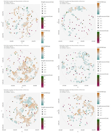
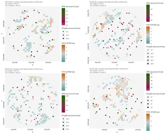
Figure A1.
Location and characteristics of the trees from field data and estimated LiDAR UC at the plot level.
Figure A1.
Location and characteristics of the trees from field data and estimated LiDAR UC at the plot level.
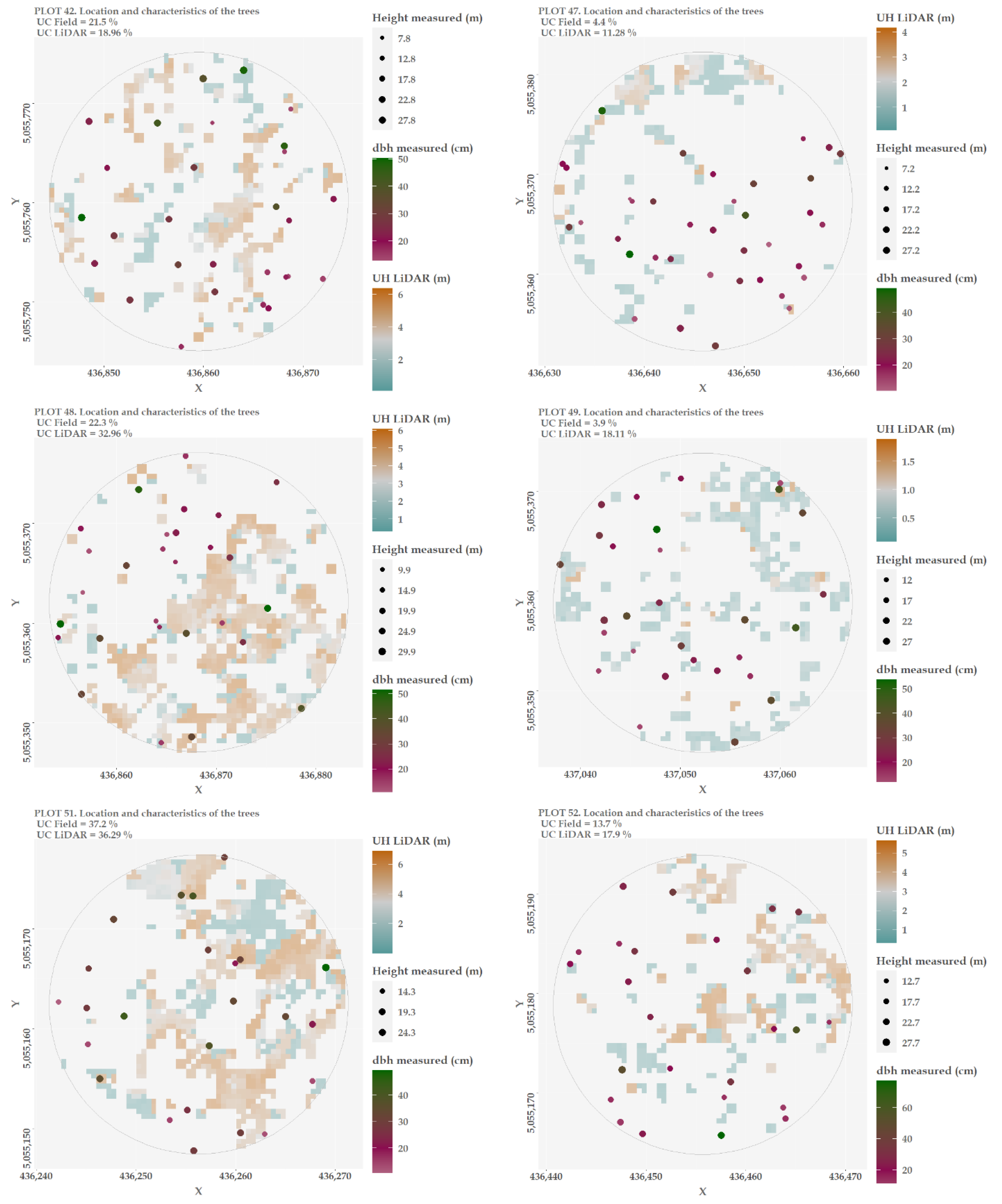
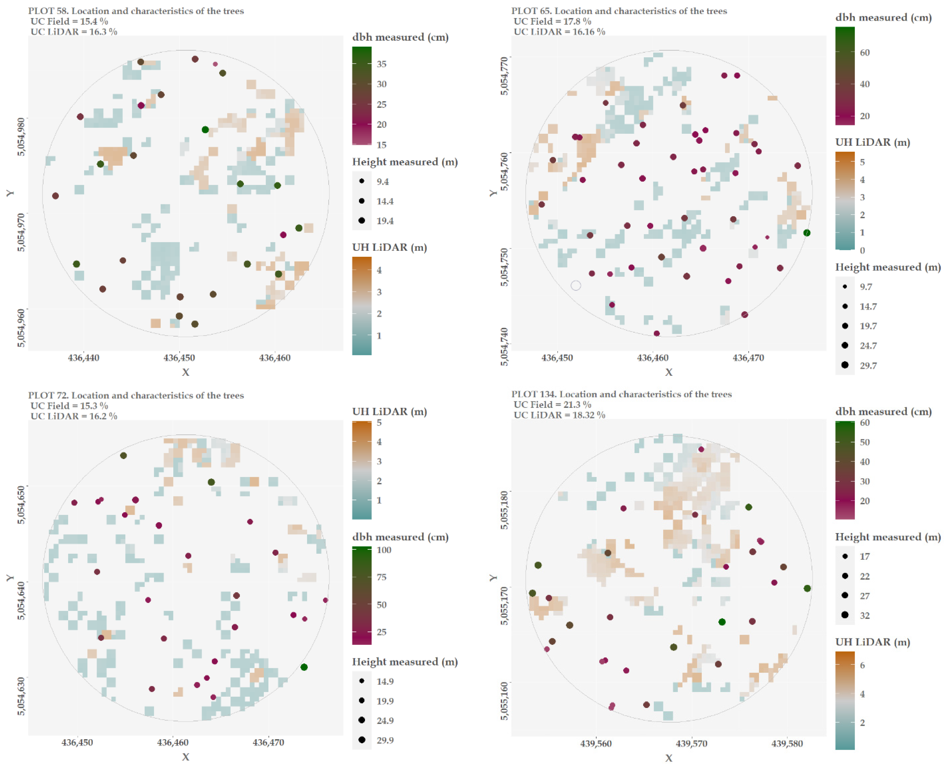
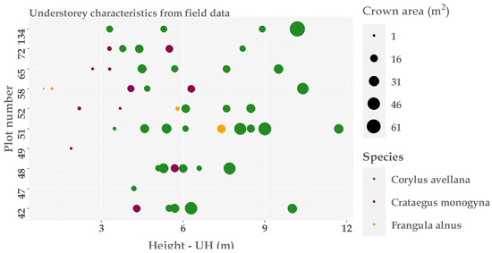
Figure A2.
Understorey characteristics (UH, crown area and shrub species) using field data at the plot level.
Figure A2.
Understorey characteristics (UH, crown area and shrub species) using field data at the plot level.
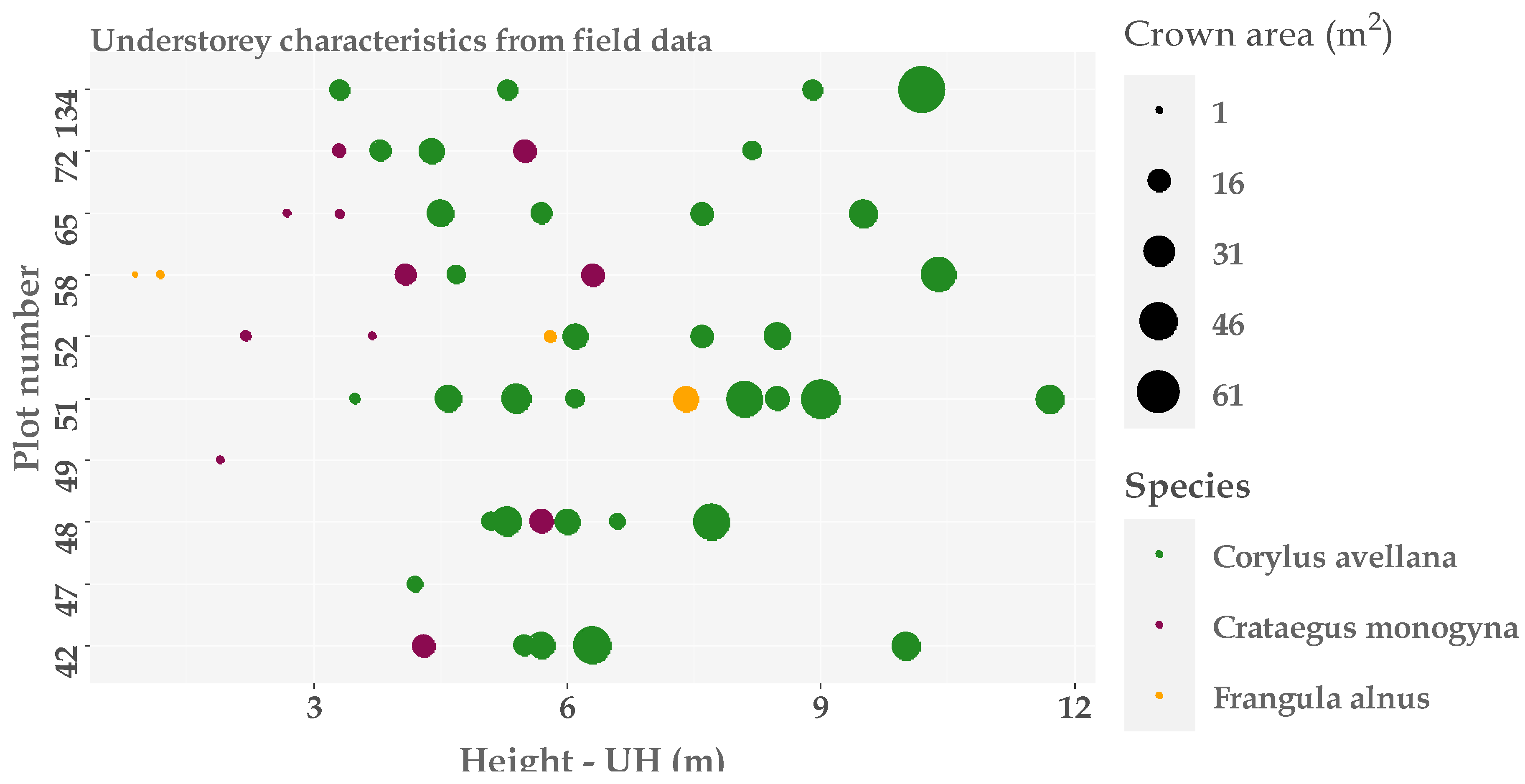
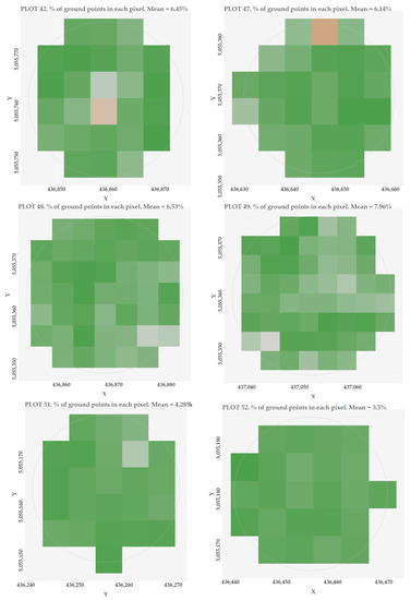
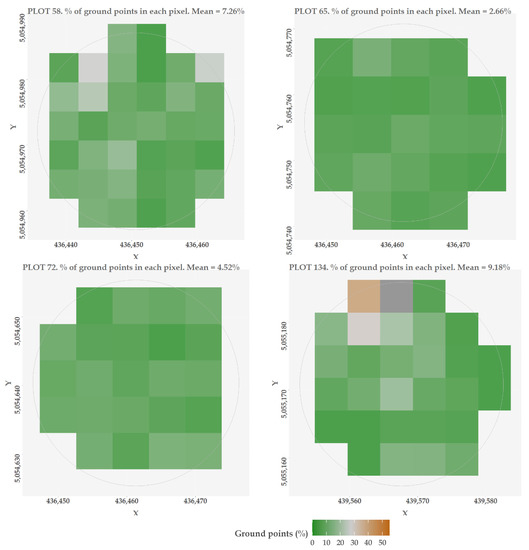
Figure A3.
Percentage of ground points at the pixel level.
Figure A3.
Percentage of ground points at the pixel level.

Appendix B. Quantitative Results

Table A1.
Statistical summary of dependent variables (HCBM) and predictor variables of the HCB models (LiDAR metrics) (see acronyms in Figure 3). Data used to create Figure 4.
| Parameter | Mean | Min | Max | SD |
|---|---|---|---|---|
| HCBMIN | 3.75 | 0.93 | 7.39 | 1.57 |
| HCBP10 | 5.63 | 2.69 | 9.91 | 1.42 |
| HCBP20 | 6.84 | 4.48 | 10.90 | 1.19 |
| HCBP25 | 7.51 | 5.29 | 12.10 | 1.40 |
| HCBP30 | 8.14 | 4.85 | 14.02 | 1.72 |
| HCBP40 | 9.92 | 6.23 | 16.24 | 2.33 |
| HCBP50 | 11.44 | 7.24 | 16.60 | 2.45 |
| HCBMEAN | 11.35 | 7.17 | 15.51 | 1.47 |
| HCBP60 | 13.07 | 8.00 | 17.32 | 2.15 |
| HCBP70 | 14.20 | 8.39 | 17.87 | 2.08 |
| HCBP75 | 14.94 | 8.76 | 19.05 | 1.91 |
| HCBP80 | 15.55 | 8.97 | 19.54 | 1.89 |
| HCBP90 | 16.77 | 11.17 | 21.10 | 1.92 |
| HCBP95 | 17.69 | 13.38 | 22.78 | 2.06 |
| HCBP99 | 18.81 | 14.35 | 24.67 | 2.17 |
| HCBMAX | 19.07 | 14.40 | 25.50 | 2.36 |
| ALLFIRST | 162.74 | 118.13 | 193.34 | 16.89 |
| ALLMEAN−FIRST | 94.30 | 62.34 | 111.57 | 8.19 |
| ALLTOTAL | 4897.66 | 1622.00 | 6063.00 | 1647.01 |
| LHAAD | 6.11 | 2.68 | 8.90 | 1.31 |
| LHL3 | −0.67 | −1.39 | 0.68 | 0.40 |
| LHMAD−MEDIAN | 4.62 | 0.94 | 9.32 | 1.71 |
| LHSK | −0.71 | −2.77 | 1.45 | 0.52 |
| LHP10 | 6.19 | 0.39 | 15.29 | 3.39 |
| LHP20 | 10.37 | 1.93 | 19.50 | 3.62 |
| LHP25 | 12.03 | 2.73 | 20.79 | 3.47 |
| LHP30 | 13.89 | 3.42 | 22.06 | 3.24 |
| LHP75 | 22.90 | 9.15 | 31.01 | 3.37 |
| B11TRC | 110.54 | 6.00 | 309.00 | 61.27 |
| B14TRC | 135.35 | 15.00 | 308.00 | 71.21 |
| B16TRC | 157.40 | 23.00 | 391.00 | 81.40 |
| B17TRC | 189.57 | 29.00 | 456.00 | 90.07 |
| B18TRC | 206.03 | 31.00 | 666.00 | 105.10 |
| B19RP | 0.06 | 0.01 | 0.20 | 0.04 |
| B21RP | 0.39 | 0.01 | 0.77 | 0.16 |

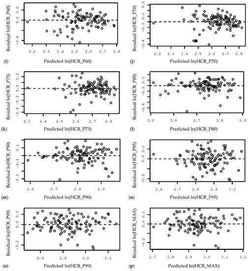
Figure A4.
Residuals versus predicted values plots of: (a) HCBMIN model; (b) HCBP10 model; (c) HCBP20 model; (d) HCBP25 model; (e) HCBP40 model; (f) HCBP40 model; (g) HCBP50 model; (h) HCBMEAN model; (i) HCBP60 model; (j) HCBP70 model; (k) HCBP75 model; (l) HCBP80 model; (m) HCBP90 model; (n) HCBP95 model; (o) HCBP99 model; and (p) HCBMAX model.

References
- Ruiz, L.Á.; Recio, J.A.; Crespo-Peremarch, P.; Sapena, M. An Object-Based Approach for Mapping Forest Structural Types Based on Low-Density LiDAR and Multispectral Imagery Based on Low-Density LiDAR and Multispectral Imagery. Geocarto Int. 2016, 33, 443–457. [Google Scholar] [CrossRef]
- Lim, K.; Treitz, P.; Wulder, M.; St-Onge, B.; Flood, M. LiDAR Remote Sensing of Forest Structure. Prog. Phys. Geogr. 2003, 27, 88–106. [Google Scholar] [CrossRef]
- Crespo-Peremarch, P.; Ruiz, L.A.; Balaguer-Beser, A. A Comparative Study of Regression Methods to Predict Forest Structure and Canopy Fuel Variables from LiDAR Full-Waveform Data. Rev. De Teledetección 2016, 45, 27–40. [Google Scholar] [CrossRef]
- Almeida, D.R.A.; Broadbent, E.N.; Zambrano, A.M.A.; Wilkinson, B.E.; Ferreira, M.E.; Chazdon, R.; Meli, P.; Gorgens, E.B.; Silva, C.A.; Stark, S.C.; et al. Monitoring the Structure of Forest Restoration Plantations with a Drone-Lidar System. Int. J. Appl. Earth Obs. Geoinf. 2019, 79, 192–198. [Google Scholar] [CrossRef]
- Sumnall, M.; Fox, T.R.; Wynne, R.H.; Thomas, V.A. Mapping the Height and Spatial Cover of Features beneath the Forest Canopy at Small-Scales Using Airborne Scanning Discrete Return Lidar. ISPRS J. Photogramm. Remote Sens. 2017, 133, 186–200. [Google Scholar] [CrossRef]
- Hill, R.A.; Broughton, R.K. Mapping the Understorey of Deciduous Woodland from Leaf-on and Leaf-off Airborne LiDAR Data: A Case Study in Lowland Britain. ISPRS J. Photogramm. Remote Sens. 2009, 64, 223–233. [Google Scholar] [CrossRef]
- Andersen, H.E.; Foster, J.R.; Reutebuch, S.E. Estimating Forest Structure Parameters Within Fort Lewis Military Reservation Using Airborne Laser Scanner (LIDAR) Data. In Proceedings of the 2nd International Precision Forestry Symposium; University of Washington, College of Forest Resources: Seattle, WA, USA, 2003; pp. 45–53. [Google Scholar]
- Latifi, H.; Hill, S.; Schumann, B.; Heurich, M.; Dech, S. Multi-Model Estimation of Understorey Shrub, Herb and Moss Cover in Temperate Forest Stands by Laser Scaner Data. Int. J. For. Res. 2017, 90, 496–514. [Google Scholar] [CrossRef][Green Version]
- Hamraz, H.; Contreras, M.A.; Zhang, J. Vertical Stratification of Forest Canopy for Segmentation of Understory Trees within Small-Footprint Airborne LiDAR Point Clouds. J. Photogramm. Remote Sens. 2017, 130, 385–392. [Google Scholar] [CrossRef]
- Fragoso, L.; Quirós, E.; Durán-Barroso, P. Variability in Estimated Runoff in a Forested Area Based on Different Cartographic Data Sources. For. Syst. 2017, 26, eRC02. [Google Scholar] [CrossRef]
- Fernández-Álvarez, M.; Armesto, J.; Picos, J. LiDAR-Based Wildfire Prevention in WUI: The Automatic Detection, Measurement and Evaluation of Forest Fuels. Forests 2019, 10, 148. [Google Scholar] [CrossRef]
- Barber, Q.E.; Bater, C.W.; Braid, A.C.R.; Coops, N.C.; Tompalski, P.; Nielsen, S.E. Airborne Laser Scanning for Modelling Understory Shrub Abundance and Productivity. For. Ecol. Manag. 2016, 377, 46–54. [Google Scholar] [CrossRef]
- Li, A.; Dhakal, S.; Glenn, N.F.; Spaete, L.P.; Shinneman, D.J.; Pilliod, D.S.; Arkle, R.S.; McIlroy, S.K. Lidar Aboveground Vegetation Biomass Estimates in Shrublands: Prediction, Uncertainties and Application to Coarser Scales. Remote Sens. 2017, 9, 903. [Google Scholar] [CrossRef]
- Aldred, A.H.; Bonnor, G.M. Application of Airborne Lasers to Forest Surveys; Canadian Forestry Service, Petawawa National Forestry Centre: Petawawa, ON, Canada, 1985; ISBN 0662138651. [Google Scholar]
- Maltamo, M.; Naesset, E.; Vauhkonen, J. Forestry Applications of Airborne Laser Scanning. Concepts and Case Studies. In Managing Forest Ecosystems; Springer: Berlin/Heidelberg, Germany, 2014; ISBN 9789402406115. [Google Scholar]
- Means, J.E.; Acker, S.A.; Fitt, B.J.; Renslow, M.; Emerson, L.; Hendrix, C.J. Predicting Forest Stand Characteristics with Airborne Scanning Lidar. Photogramm. Eng. Remote Sens. 2000, 66, 1367–1371. [Google Scholar]
- Maltamo, M.; Karjalainen, T.; Repola, J.; Vauhkonen, J. Incorporating Tree- and Stand-Level Information on Crown Base Height into Multivariate Forest Management Inventories Based on Airborne Laser Scanning. Silva Fenn. 2018, 52, 10006. [Google Scholar] [CrossRef]
- Pearse, G.D.; Watt, M.S.; Dash, J.P.; Stone, C.; Caccamo, G. Comparison of Models Describing Forest Inventory Attributes Using Standard and Voxel-Based Lidar Predictors across a Range of Pulse Densities. Int. J. Appl. Earth Obs. Geoinf. 2019, 78, 341–351. [Google Scholar] [CrossRef]
- Riaño, D.; Chuvieco, E.; Condés, S.; González-Matesanz, J.; Ustin, S.L. Generation of Crown Bulk Density for Pinus Sylvestris L. from Lidar. Remote Sens. Environ. 2004, 92, 345–352. [Google Scholar] [CrossRef]
- Andersen, H.; Mcgaughey, R.J.; Reutebuch, S.E. Estimating Forest Canopy Fuel Parameters Using LIDAR Data. Remote Sens. Environ. 2005, 94, 441–449. [Google Scholar] [CrossRef]
- Engelstad, P.S.; Falkowski, M.; Wolter, P.; Poznanovic, A.; Johnson, P. Estimating Canopy Fuel Attributes from Low-Density LiDAR. Fire 2019, 2, 38. [Google Scholar] [CrossRef]
- García, M.; Saatchi, S.; Casas, A.; Koltunov, A.; Ustin, S.; Ramirez, C.; Garcia-Gutierrez, J.; Balzter, H. Quantifying Biomass Consumption and Carbon Release from the California Rim Fire by Integrating Airborne LiDAR and Landsat OLI Data. J. Geophys. Res. Biogeosci. 2017, 122, 340–353. [Google Scholar] [CrossRef]
- Almeida, D.R.A.; Stark, S.C.; Chazdon, R.; Nelson, B.W.; Cesar, R.G.; Meli, P.; Gorgens, E.B.; Duarte, M.M.; Valbuena, R.; Moreno, V.S.; et al. The Effectiveness of LiDAR Remote Sensing for Monitoring Forest Cover Attributes and Landscape Restoration. For. Ecol. Manag. 2019, 438, 34–43. [Google Scholar] [CrossRef]
- Wing, B.M.; Ritchie, M.W.; Boston, K.; Cohen, W.B.; Gitelman, A.; Olsen, M.J. Prediction of Understory Vegetation Cover with Airborne LiDAR in an Interior Ponderosa Pine Forest. Remote Sens. Environ. 2012, 124, 730–741. [Google Scholar] [CrossRef]
- Goodwin, N.R. Assessing Understorey Structural Characteristics in Eucalypt Forests: An Investigation of LiDAR Techniques; University of New South Wales: Sydney, NSW, Australia, 2006. [Google Scholar]
- Glenn, N.F.; Spaete, L.P.; Sankey, T.T.; Derryberry, D.R.; Hardegree, S.P.; Mitchell, J.J. Errors in LiDAR-Derived Shrub Height and Crown Area on Sloped Terrain. J. Arid. Environ. 2011, 75, 377–382. [Google Scholar] [CrossRef]
- Sankey, T.T.; Mcvay, J.; Swetnam, T.L.; McClaran, M.P.; Heilman, P.; Nichols, M. UAV Hyperspectral and Lidar Data and Their Fusion for Arid and Semi-Arid Land Vegetation Monitoring. Remote Sens. Ecol. Conserv. 2018, 4, 20–33. [Google Scholar] [CrossRef]
- Prošek, J.; Šímová, P. UAV for Mapping Shrubland Vegetation: Does Fusion of Spectral and Vertical Information Derived from a Single Sensor Increase the Classification Accuracy? Int. J. Appl. Earth Obs. Geoinf. 2019, 75, 151–162. [Google Scholar] [CrossRef]
- Martinuzzi, S.; Vierlin, L.A.; Gould, W.A.; Falkowski, M.J.; Evans, J.S.; Hudak, A.T.; Vierling, K.T. Mapping Snags and Understory Shrubs for a LiDAR-Based Assessment of Wildlife Habitat Suitability. Remote Sens. Environ. 2009, 119, 2533–2546. [Google Scholar] [CrossRef]
- Venier, L.A.; Swystun, T.; Mazerolle, M.J.; Kreutzweiser, D.P.; WainioKeizer, K.L.; McIlwrick, K.A.; Woods, M.E.; Wang, X. Modelling Vegetation Understory Cover Using LiDAR Metrics. PLoS ONE 2019, 27, e0220096. [Google Scholar] [CrossRef] [PubMed]
- Fragoso-Campón, L.; Quirós, E.; Mora, J.; Gutiérrez, J.A.; Durán-Barroso, P. Accuracy Enhancement for Land Cover Classification Using LiDAR and Multitemporal Sentinel 2 Images in a Forested Watershed. In Proceedings of the Envifonment, Green Technology and Engineering International Conference, Semarang, Indonesia, 18 October 2018; pp. 2–5. [Google Scholar]
- Jarron, L.R.; Coops, N.C.; Mackenzie, W.H.; Tompalski, P.; Dykstra, P. Detection of Sub-Canopy Forest Structure Using Airborne LiDAR. Remote Sens. Environ. 2020, 244, 111770. [Google Scholar] [CrossRef]
- Su, J.G.; Bork, E.W. Characterization of Diverse Plant Communities in Aspen Parkland Rangeland Using LiDAR Data. Appl. Veg. Sci. 2007, 10, 407–416. [Google Scholar] [CrossRef]
- Ritchie, M.W.; Hann, D.W. Equations for Predicting Height to Crown Base for Fourteen Tree Species in Southwest Oregon; Oregon State University, Forest Research Laboratory (USA): Corvallis, OR, USA, 1987; Volume 50. [Google Scholar]
- Rijal, B.; Weiskittel, A.R.; Kershaw, J.A. Development of Height to Crown Base Models for Thirteen Tree Species of the North American Acadian Region. For. Chron. 2012, 88, 60–73. [Google Scholar] [CrossRef]
- Fu, L.; Zhang, H.; Sharma, R.P.; Pang, L.; Wang, G. A Generalized Nonlinear Mixed-Effects Height to Crown Base Model for Mongolian Oak in Northeast China. For. Ecol. Manag. 2017, 384, 34–43. [Google Scholar] [CrossRef]
- Sharma, R.P.; Vacek, Z.; Vacek, S.; Podrázský, V.; Jansa, V. Modelling Individual Tree Height to Crown Base of Norway Spruce (Picea Abies (L.) Karst.) and European Beech (Fagus Sylvatica L.). PLoS ONE 2017, 12, e0186394. [Google Scholar] [CrossRef] [PubMed]
- Stefanidou, A.; Gitas, I.Z.; Korhonen, L.; Stavrakoudis, D.; Georgopoulos, N. LiDAR-Based Estimates of Canopy Base Height for a Dense Uneven-Aged Structured Forest. Remote Sens. 2020, 12, 1565. [Google Scholar] [CrossRef]
- Balenović, I.; Jurjević, L.; Milas, A.S.; Gašparović, M.; Ivanković, D.; Seletković, A. Testing the Applicability of the Official Croatian DTM for Normalization of UAV-Based DSMs and Plot-Level Tree Height Estimations in Lowland Forests. Croat. J. For. Eng. 2019, 40, 163–174. [Google Scholar]
- Ostrogović Sever, M.Z.; Alberti, G.; Delle Vedove, G.; Marjanović, H. Temporal Evolution of Carbon Stocks, Fluxes and Carbon Balance in Pedunculate Oak Chronosequence under Close-to-Nature Forest Management. Forests 2019, 10, 814. [Google Scholar] [CrossRef]
- Klepac, D.; Fabijanić, G. Management of Pedunculate Oak Forest. In Monography: Pedunculate Oak in Croatia; Klepac; Croatian Academy of Science and Art and Croatian Forests Ltd.: Zagreb, Croatia, 1996; pp. 257–272. [Google Scholar]
- Croatian Forests Ltd. Forest Management Area Plan for the Republic of Croatia for the Period 2016–2025; Croatian Forests Ltd.: Zagreb, Croatia, 2016. [Google Scholar]
- Michailoff, I. Zahlenmässiges Verfahren Für Die Aus- Führung Der Bestandeshöhenkurven. Cbl. Und Thar. Forstl. Jahrb. 1943, 6, 273–279. [Google Scholar]
- Martín-García, S.; Balenović, I.; Jurjević, L.; Lizarralde, I.; Indir, K.; Ponce, R.A. Height to Crown Base Modelling for the Main Tree Species in an Even-Aged Pedunculate Oak Forest: A Case Study from Central Croatia. South-East Eur. For. 2021, 12, 1–11. [Google Scholar] [CrossRef]
- ASPRS LAS Specification 1.4—R15; The American Sciety for Photogrammetry & Remote Sensign. ASPRS: Bethesda, MD, USA, 2019; 47p.
- TerraSolid Ltd. TerraScan—Software for LiDAR Data Processing and 3D Vector Data Creation; TerraSolid Ltd.: Helsinki, Finland, 2012. [Google Scholar]
- Buján, S.; González-Ferreiro, E.M.; Cordero, M.; Miranda, D. PpC: A New Method to Reduce the Density of Lidar Data. Does It Affect the DEM Accuracy? Photogramm. Rec. 2019, 34, 304–329. [Google Scholar] [CrossRef]
- Alonso, R.; Lizarralde, I.; Rodríguez-Puerta, F.; Pérez-Rodríguez, F. EasyLaz 1.0: Patent SO-8/2018 2018. Available online: https://www.researchgate.net/publication/324983460_easyLaz (accessed on 17 March 2022).
- McGaughey, R.J. FUSION/LDV: Software for LIDAR Data Analysis and Visualization; V4.20; USDA: Seatle, WA, USA, 2018; 212p, Available online: http://forsys.sefs.uw.edu/fusion/fusion_overview.html (accessed on 17 March 2022).
- Kraus, K.; Pfeifer, N. Determination of Terrain Models in Wooded Areas with Airborne Laser Scanner Data. ISPRS J. Photogramm. Remote Sens. 1998, 53, 193–203. [Google Scholar] [CrossRef]
- R Core Team. R: A Language and Environment for Statistical Computing; R Core Team: Vienna, Austria, 2019. [Google Scholar]
- Lumley, T. Leaps: Regression Subset Selection. R Package Version 3.0. 2017. Available online: https://cran.r-project.org/package=leaps (accessed on 17 March 2022).
- Sprugel, D.G. Correcting for Bias in Log-Transformed Allometric Equations. Ecology 1983, 64, 209–210. [Google Scholar] [CrossRef]
- Fox, J.; Weisberg, S. An {R} Companion to Applied Regression, 3rd ed.; R Core Team: Vienna, Austria, 2019. [Google Scholar]
- Maguya, A.S.; Tegel, K.; Junttila, V.; Kauranne, T.; Korhonen, M.; Burns, J.; Leppanen, V.; Sanz, B. Moving Voxel Method for Estimating Canopy Base Height from Airborne Laser Scanner Data. Remote Sens. 2015, 7, 8950–8972. [Google Scholar] [CrossRef]
- Luo, L.; Zhai, Q.; Su, Y.; Ma, Q.; Kelly, M.; Guo, Q. Simple Method for Direct Crown Base Height Estimation of Individual Conifer Trees Using Airborne LiDAR Data. Opt. Express 2018, 26, 767–781. [Google Scholar] [CrossRef] [PubMed]
- Skowronski, N.; Clark, K.; Nelson, R.; Hom, J.; Patterson, M. Remotely Sensed Measurements of Forest Structure and Fuel Loads in the Pinelands of New Jersey. Remote Sens. Environ. 2007, 108, 123–129. [Google Scholar] [CrossRef]
- Morsdorf, F.; Mårell, A.; Koetz, B.; Cassagne, N.; Pimont, F.; Rigolot, E.; Allgöwer, B. Discrimination of Vegetation Strata in a Multi-Layered Mediterranean Forest Ecosystem Using Height and Intensity Information Derived from Airborne Laser Scanning. Remote Sens. Environ. 2010, 114, 1403–1415. [Google Scholar] [CrossRef]
- Riaño, D.; Meier, E.; Allgöwer, B.; Chuvieco, E.; Ustin, S.L. Modeling Airborne Laser Scanning Data for the Spatial Generation of Critical Forest Parameters in Fire Behavior Modeling. Remote Sens. Environ. 2003, 86, 177–186. [Google Scholar] [CrossRef]
- Gopalakrishnan, R.; Thomas, V.A.; Wynne, R.H.; Coulston, J.W.; Fox, T.R. Shrub Detection Using Disparate Airborne Laser Scanning Acquisitions over Varied Forest Cover Types. Int. J. Remote Sens. 2017, 39, 1220–1242. [Google Scholar] [CrossRef]
Publisher’s Note: MDPI stays neutral with regard to jurisdictional claims in published maps and institutional affiliations. |
© 2022 by the authors. Licensee MDPI, Basel, Switzerland. This article is an open access article distributed under the terms and conditions of the Creative Commons Attribution (CC BY) license (https://creativecommons.org/licenses/by/4.0/).

