Fast Superpixel-Based Non-Window CFAR Ship Detector for SAR Imagery

Abstract

Ship detection in high-resolution synthetic aperture radar (SAR) images has attracted great attention. As a popular method, a constant false alarm rate (CFAR) detection algorithm is widely used. However, the detection performance of CFAR is easily affected by speckle noise. Moreover, the sliding window technique cannot effectively differentiate between clutter and target pixels and easily leads to a high computation load. In this paper, we propose a new superpixel-based non-window CFAR ship detection method for SAR images, which introduces superpixels to CFAR detection to resolve the aforementioned drawbacks. Firstly, our previously proposed fast density-based spatial clustering of applications with noise (DBSCAN) superpixel generation method is utilized to produce the superpixels for SAR images. With the assumption that SAR data obeys gamma distribution, the superpixel dissimilarity is defined. Then, superpixels can be accurately used to estimate the clutter parameters for the tested pixel, even in the multi-target situations, avoiding the drawbacks of the sliding window in the traditional CFAR. Moreover, a local superpixel contrast is proposed to optimize CFAR detection, which can eliminate numerous clutter false alarms, such as man-made urban areas and low bushes. Experimental results with real SAR images indicate that the proposed method can achieve ship detection with a higher speed and accuracy in comparison with other state-of-the-art methods.

1. Introduction

Synthetic aperture radar (SAR) is a popular remote sensing sensor due to its relatively high resolution and all-time and all-weather imaging capability, and it is widely used in various monitoring tasks. Ship detection is one of the important applications for the ocean monitoring, which has attracted great attention from scholars. Constant false alarm rate (CFAR) algorithms are widely used target detection methods due to their simplicity and adaptive ability. For the reason that different kinds of background clutter have different statistical distributions, a large number of CFAR detectors have been proposed with different local statistics. For example, commonly used CFAR detectors include the cell-averaging CFAR (CA-CFAR) detector [1], largest CFAR (GO-CFAR) detector [2], two-parameter CFAR (TP-CFAR) detector [3], order-statistic CFAR detector (OS-CFAR) [4], and smallest CFAR (SO-CFAR) detector, etc.

These CFAR detectors can work well in situations where a single target exists among locally homogeneous clutter. Nevertheless, when using a local sliding window to estimate local statistics of the sea background, there is the inevitable problem of CFAR detectors. When multiple targets exist, the sea clutter obtained by using the local window may contain other target pixels [5,6,7]. Therefore, parameters of the clutter’s distribution would be incorrectly estimated, causing a deterioration of the detection performance [8,9]. To overcome this drawback, many efforts were devoted to improving the conventional CFAR algorithm. Gao et al. [10] proposed a censoring approach with an initial detection to exclude the outliers and achieve accurate distribution parameters for the background clutter. However, the censoring depth is difficult to determine. After that, Cui et al. [8] proposed an iterative censoring scheme for target detection with SAR imagery, which iteratively updates the target maps for censoring. Based on this idea, An et al. [9] proposed an improved iterative censoring detection scheme to accelerate the CFAR detection. Although the performance is improved, the computational burden is too heavy due to the iterative scheme and the sliding window technique. Hou et al. [11] proposed a multilayer CFAR, which could overcome the holes and fracture in the traditional detected results using the CFAR method. Although the detection time is greatly reduced for the reason that global CFAR is used instead of local CFAR, the false alarm rate reamins relatively high. Leng et al. [12] proposed a bilateral CFAR, which could reduce the influence of SAR ambiguities and sea clutter by considering the ship spatial distribution of SAR images.

However, with the increase in SAR image resolution, due to the data acquired by the TerraSAR, ICEYE sensors, etc., new challenges for ship target detection arise, and the conventional CFAR detectors may suffer from severe performance deterioration. For example, the serious speckle of high-resolution SAR image increases the probability of a false alarm. Moreover, in high-resolution SAR images, a ship target usually contains a multiple number of independent strong scatters [10,13]. After CFAR detection, a ship target is likely to be composed of distributed pixels which cannot form a connected region, leading to the loss of information of structure and shape of the ships. Moreover, it is difficult to eliminate the numerous man-made clutter false alarms, such as in urban areas by only considering the pixel intensity differences between the ships and sea clutter [14].

Nowadays, the superpixel segmentation is applied to SAR data processing [15,16]. A ship target can contain one or several connected superpixels after superpixel segmentation, which can offer more useful statistic and structure information than the pixels. Therefore, several superpixel-based ship detection methods have been studied. Combined with a modified two parameter CFAR detector, Yu et al. [7] used superpixels to accurately obtain the clutter distribution parameters and then perform CFAR detection. Pappas et al. [6] utilized superpixels instead of rectangular sliding windows to define CFAR guard areas and background. The aim is to achieve better target exclusion from the background band and reduced false detections. Li et al. [13] regarded superpixels as the basic processing unit instead of a single pixel for SAR image ship detection, which is superior to the traditional CFAR method in terms of detection performance and computational efficiency. Liu et al. [17] used multi-scale superpixels to segment the SAR image by sea and land, with a combination of CFAR detectors to detect the shore ship targets. Li et al. [18] divided superpixels into pure superpixels and hybrid superpixels, and adaptively selected a sufficient number of pure clutter superpixels for detection threshold estimation.

Although the aforementioned superpixel-based CFAR detectors can improve the ship detection performance, most of the methods are implemented with the sliding window scheme [2,10], i.e., the window is moving over all superpixels in the image to adaptively select clutter superpixels, leading to a relatively high computation load, especially for a high-resolution SAR image with a large size. In addition, the numerous clutter false alarms are hardly eliminated, causing the detection results to have a high false alarm rate.

Recently, many deep-learning-based ship detection methods have been proposed for SAR images, such as the CenterNet [19] and multidimensional domain deep learning network [20], etc. For instance, Zhang et al. [21] considered the idea of the You Only Look Once (YOLO) series algorithm and proposed a grid convolutional neural network (G-CNN) for SAR ship detection. Wang et al. [22] adjusted the hyper-parameters of RetinaNet for SAR ship detection. Zhang et al. [23] considered combining the multi-scale detection strategy, concatenation mechanism, and anchor box idea into a depth-wise separable convolution neural network (DS-CNN) to achieve SAR ship detection. These methods tried to use large SAR ship datasets, such as the SAR ship detection data set (SSDD) [24] and OpenSARship dataset [25], to train the deep learning model and achieve ship detection for input SAR images. Therefore, the detection procedure highly depended on the dataset for the training.

In order to resolve the above problems, this paper applies superpixels to CFAR ship detection, and proposes a superpixel-based non-window fast CFAR (SP-NW-CFAR) ship detector for SAR images, such as the TerraSAR X band, Sentinel-1 C band and GF-3 C band images. Our previously proposed fast density-based spatial clustering of applications with noise (DBSCAN) superpixel generation method [26] was utilized to produce the superpixels for SAR images. Then, we defined the superpixel dissimilarity to automatically select the pure clutter superpixels, which estimated the clutter parameters for each tested pixel, even in the multi-target situations. Moreover, a local superpixel contrast was also defined to optimize the CFAR detection, which could eliminate the numerous clutter false alarms. The main contributions of the proposed method are as follows:

(1) We introduce the superpixels to the CFAR detection, thus avoiding the operation of the sliding window;

(2) The superpixel dissimilarity is used to select the pure sea clutter superpixels, making the clutter’s distribution parameter estimation more accurate. Moreover, the pixels within one superpixel share the same clutter distribution parameters, which results in a very fast CFAR detection;

(3) A local superpixel contrast is used to optimize the CFAR detection, which can reduce the false alarm rate.

The remainder of this paper is organized as follows. The related work, including the CFAR detector and superpixel generation method is briefly introduced in Section 2. Section 3 presents a detailed description of the superpixel-based non-window fast CFAR method. Then, the experimental results with real SAR images are provided in Section 4. Some discussions are exhibited in Section 5. Conclusions are provided in Section 6.

2. Related Works

2.1. Brief Review on the CFAR Detectors

The CFAR detector is an adaptive threshold detector, which estimates the statistical distribution of sea clutter around the target based on a hypothetical background probability density function $p\left(x\right)$, so as to maintain a constant acceptable probability of false alarms $P_{fa}$ [2]. The CFAR detection compares the gray intensity of a single pixel with a certain threshold to determine whether the pixel belongs to the ship target. Three elements are required to determine this threshold, which are the pre-set false alarm rate $P_{fa}$, the assumed clutter statistical model, and the local sliding window [2,10]. The traditional CFAR detector traverses all pixels in the SAR image through a sliding window to achieve pixel-by-pixel target detection. At present, the most commonly used CFAR sliding window is a hollow sliding window, which can be divided into three components from the inside to the outside, namely the target area, the guard area and the clutter area [10,11].

Given the false alarm rate $P_{fa}$, and the probability density function (PDF) of the clutter $p\left(x\right)$ is: [10]

$$P_{fa}={{\displaystyle \int }}_T^{\infty }p\left(x\right)dx$$

(1)

Then, the detection threshold $T$ can be obtained and the target detection decision can be expressed as:

$$\left\{\begin{array}{c}x>T, \mathrm{the} \mathrm{detection} \mathrm{pixel} \mathrm{belongs} \mathrm{to} \mathrm{the} \mathrm{target} \\ x\le T, \mathrm{the} \mathrm{detection} \mathrm{pixel} \mathrm{belongs} \mathrm{to} \mathrm{the} \mathrm{background}\end{array}\right.$$

(2)

where $x$ is intensity of the pixels in the SAR image. Note that typical statistical models used in the CFAR detectors include distributions, such as the gamma, Weibull, Rayleigh, and K-distributions [10]. Some complicated distribution models that computationally promote the clutter modeling accuracy include the generalized heavy-tailed Rayleigh [27], a mixture of Rayleigh models [28], and the generalized gamma and generalized gamma mixture models [29]. The gamma distribution can be used for the clutter modeling of high-resolution SAR intensity data [5,7] with the PDF calculated as:

$$f\left(x\right)=\frac{{\beta }^{\alpha }}{\mathsf{\Gamma }\left(\alpha \right)}{x}^{\alpha -1}{e}^{-\beta x}, \beta ,\alpha ,x>0$$

(3)

where $\alpha$ and $\beta$ denote the shape and inverse scale parameter, respectively. $\mathsf{\Gamma }\left(·\right)$ represents the gamma function. According to the method of log cumulants in [30], the distribution parameters $\alpha$ and $\beta$ can be calculated as follows:

$$\left\{\begin{array}{c}\frac{1}{N}{\displaystyle {\displaystyle \sum }_{i=1}^N}log{x}_i=-log\beta +\mathsf{\Psi }\left(\alpha \right)\\ \frac{1}{N}{\displaystyle {\displaystyle \sum }_{i=1}^N}{\left(\frac{1}{N}{\displaystyle {\displaystyle \sum }_{i=1}^N}log{x}_i-log{x}_i\right)}^2=\mathsf{\Psi }\left(1,\alpha \right)\end{array}\right.$$

(4)

2.2. Superpixel Generation Methods for SAR Images

The simple linear iterative clustering (SLIC) [31] is a popular superpixel generation method for natural images. However, compared with natural images, the single-channel SAR intensity images only have gray level information. Moreover, due to the speckle noise, the superpixel generation performance is not satisfactory by directly applying the SLIC to high-resolution SAR images. Therefore, the original SLIC method has been adapted for SAR images to cope with the aforementioned problems [13,15,32,33]. Most of these methods replace the Euclidean distance in the original SLIC with the dissimilarity measure for SAR image pixels. For instance, in [15], the pixel intensity and local information similarity is defined for the SAR images, which correlates with the speckle noise. Therefore, the SLIC algorithm can be adapted for SAR image superpixel generation. Apart from the redesigned pixel dissimilarity, some methods consider the SAR image homogeneity and introduce it into the distance measure, making the superpixel generation adaptive to the SAR image scene, such as the method in [34].

3. The Proposed CFAR Detector for SAR Imagery

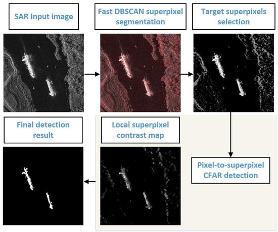
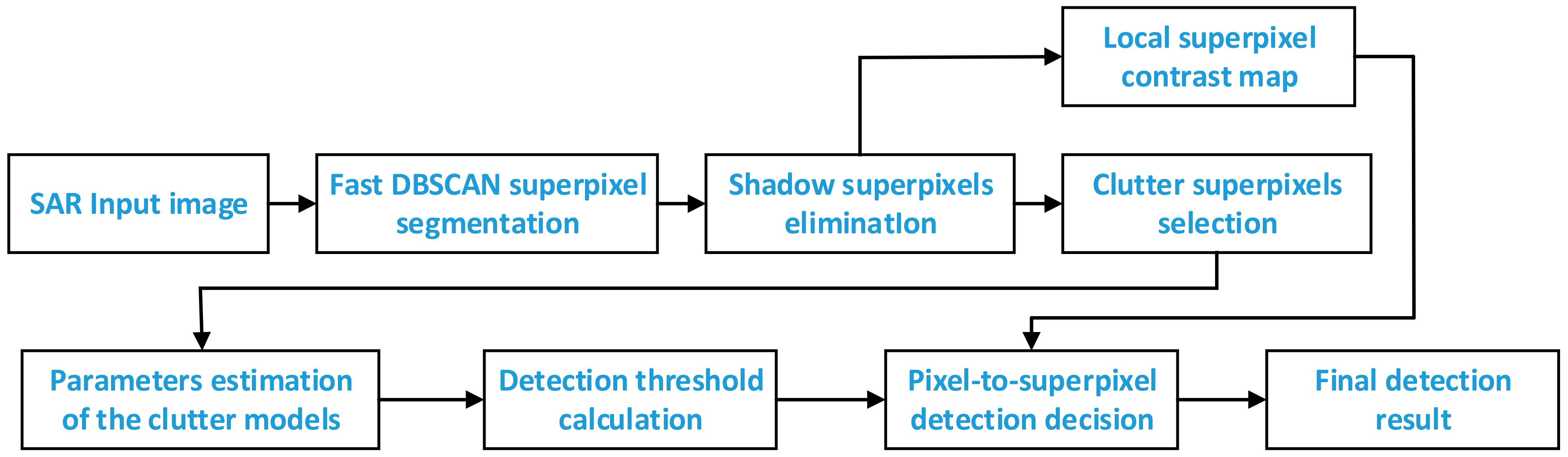
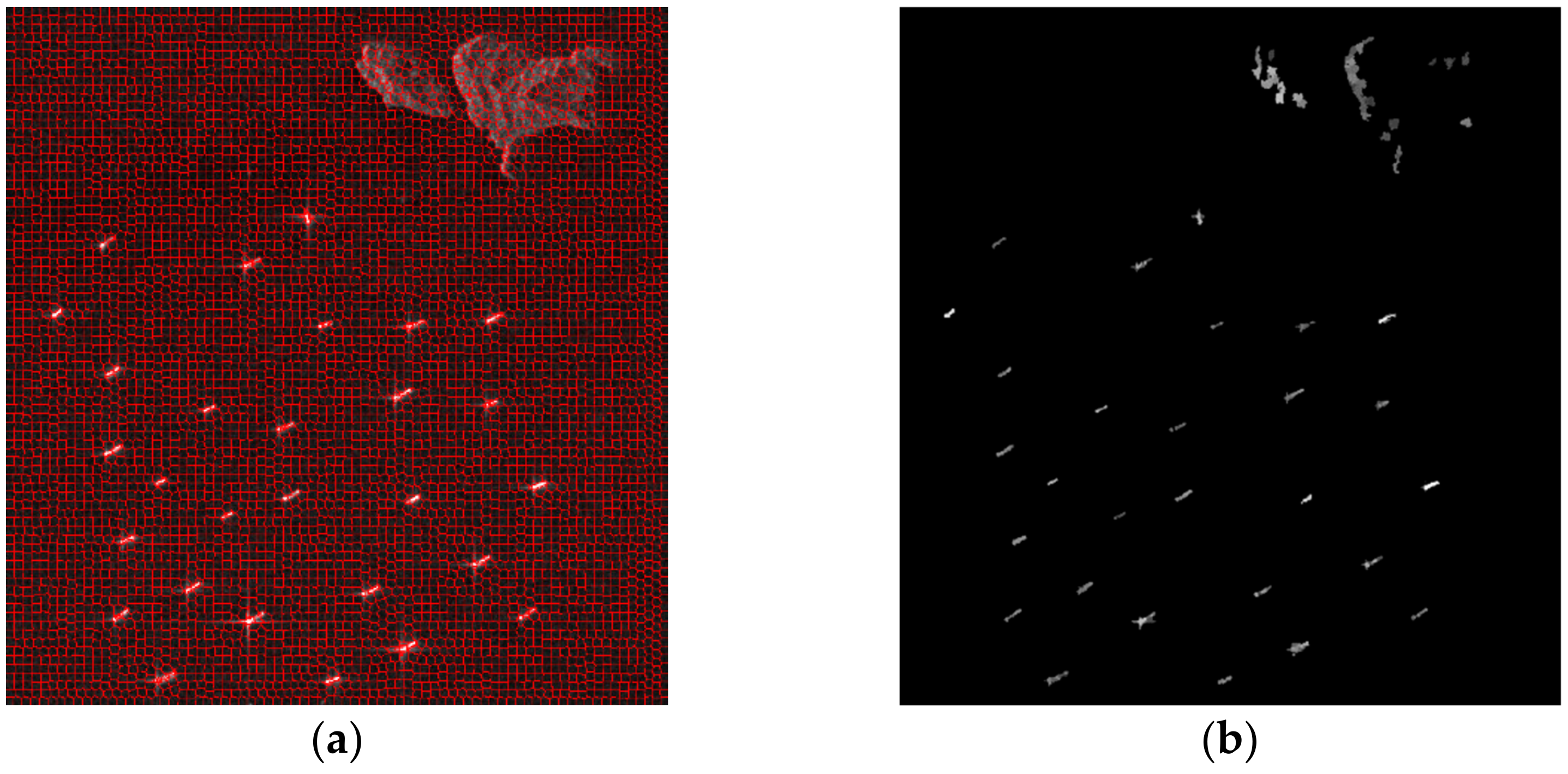
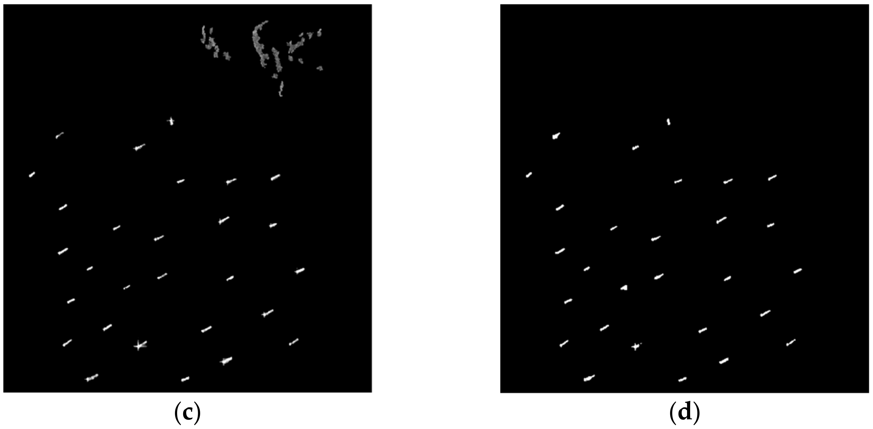
This section gives the details of our proposed superpixel-based non-window fast CFAR method, which has a flowchart as in Figure 1. The original SAR image is firstly segmented by our previous proposed fast DBSCAN superpixel generation method. Then, we define the superpixel dissimilarity to automatically select the pure clutter superpixels, which can actually estimate the clutter parameters for each under test pixel, even in the multi-target situations. It is worth pointing out that the shadow superpixels should be removed since they have no radar echoes but only noises, which may disturb the clutter parameter estimation and degrade the detection performance. After that, a local superpixel contrast is also defined to optimize the CFAR detection, which can eliminate the numerous clutter false alarms. Since the under-test pixels in the same superpixel share the same background clutter model parameters, no pixel-by-pixel clutter parameter estimation is required, making the detection efficient. More importantly, our proposed CFAR detection is not performed on all pixels but only on the potential target superpixels, which can achieve fast target detection.

3.1. Superpixel Segmentation with the Fast DBSCAN Algorithm

This subsection gives the brief description of the superpixel segmentation strategy in our method. The original fast DBSCAN superpixel generation algorithm in [26] consists of two stages, i.e., fast clustering and merging. In the clustering stage, a new adaptive pixel dissimilarity measure for SAR image is proposed and then the DBSCAN strategy is optimized. In the merging stage, based on the initial superpixels, a new superpixel dissimilarity measure is defined, which can merge the small local superpixels into their neighborhood superpixels, making the final superpixel segmentation compact and regular. Note that the edge information of SAR images is considered in the pixel dissimilarity and superpixel dissimilarity, which can maintain the image boundaries during superpixel generation. However, for simplicity, we do not consider the edge penalty for the superpixel generation in this paper, which can accelerate this stage. Thus, the pixel dissimilarity $\mathsf{\Omega }\left(i,j\right)$ is defined as: [26]

$$\mathsf{\Omega }\left(i,j\right)=\delta \left(i,j\right)+\left|\mathcal{H}\left(i\right)-\mathcal{H}\left(j\right)\right|·\delta \left(k,j\right)$$

(5)

where the intensity dissimilarity $\delta \left(i,j\right)$ of pixels $i$ and $j$ can be defined based on the likelihood ratio test statistic using two $5\times 5$ patches $P_i$ and $P_j$ which are centering the two pixels as [26]:

$$\delta \left(i,j\right)=2M·L·ln\frac{{\overline{I}}_{P_i}+{\overline{I}}_{P_j}}{2\sqrt{{\overline{I}}_{P_i}·{\overline{I}}_{P_j}}}$$

(6)

The ${\overline{I}}_{P_i}$ and ${\overline{I}}_{P_j}$ indicate the average intensity of two patches. $M$ is the number of pixels in the patch. $L$ is the number of looks of the SAR images. The $\mathcal{H}\left(i\right)$ and $\mathcal{H}\left(j\right)$ in Equation (5) denote the homogeneity of two pixels, which can be calculated by the coefficient of variation of SAR image. The $k$ in Equation (5) denotes a seed, which is the center of each generated superpixel. The clustering stage seems like region growing, which will stop until the termination condition is satisfied. Then, the initial superpixels are generated after getting enough pixels with different labels.

In order to eliminate the small superpixels, we then perform the merging stage, which merges the superpixels and eliminate small fragments, leading to final superpixel results. If the number of pixels within one initial superpixel is less than a threshold, we will merge it with its neighbor initial superpixel which has the lowest dissimilarity. The superpixel dissimilarity $\mathsf{\Omega }\left(S{P}_m,S{P}_n\right)$ is defined as:

$$\mathsf{\Omega }\left(S{P}_m,S{P}_n\right)=\sigma \left(S{P}_m,S{P}_n\right)+\left|\mathcal{H}\left(S{P}_m\right)-\mathcal{H}\left(S{P}_n\right)\right|$$

(7)

$$\sigma \left(S{P}_m,S{P}_n\right)=2·min\left(size\left(S{P}_m\right),size\left(S{P}_n\right)\right)·L\cdot ln\frac{{\overline{I}}_{S{P}_m}+{\overline{I}}_{S{P}_n}}{2\sqrt{{\overline{I}}_{S{P}_m}·{\overline{I}}_{S{P}_n}}}$$

(8)

where $size\left(·\right)$ indicates the superpixel size. We can see that the superpixel dissimilarity considers intensity and homogeneity information. Two superpixels have similar intensity values and homogeneity will be easily merged. Further details of the implementation of the fast DBSCAN superpixel generation method can be found in [26].

3.2. Shadow Superpixels Elimination

Considering that the shadow areas in the SAR images have no radar echoes, therefore, there is no texture information in the SAR images. The shadow superpixels would disturb the estimation of the clutter distributions, resulting in degrading the CFAR detection performance. Thus in this paper, we eliminate the shadow superpixels before the selection of clutter superpixels. Generally, we can set a threshold $T_{sh}$ according to the average intensity values of the shadow areas in the training SAR data. The superpixels whose average pixel intensities lower than $T_{sh}$ can be regarded as shadow superpixels, which should be removed from the superpixel set.

3.3. Clutter Superpixels Selection and Local Superpixel Contrast Map Claculation

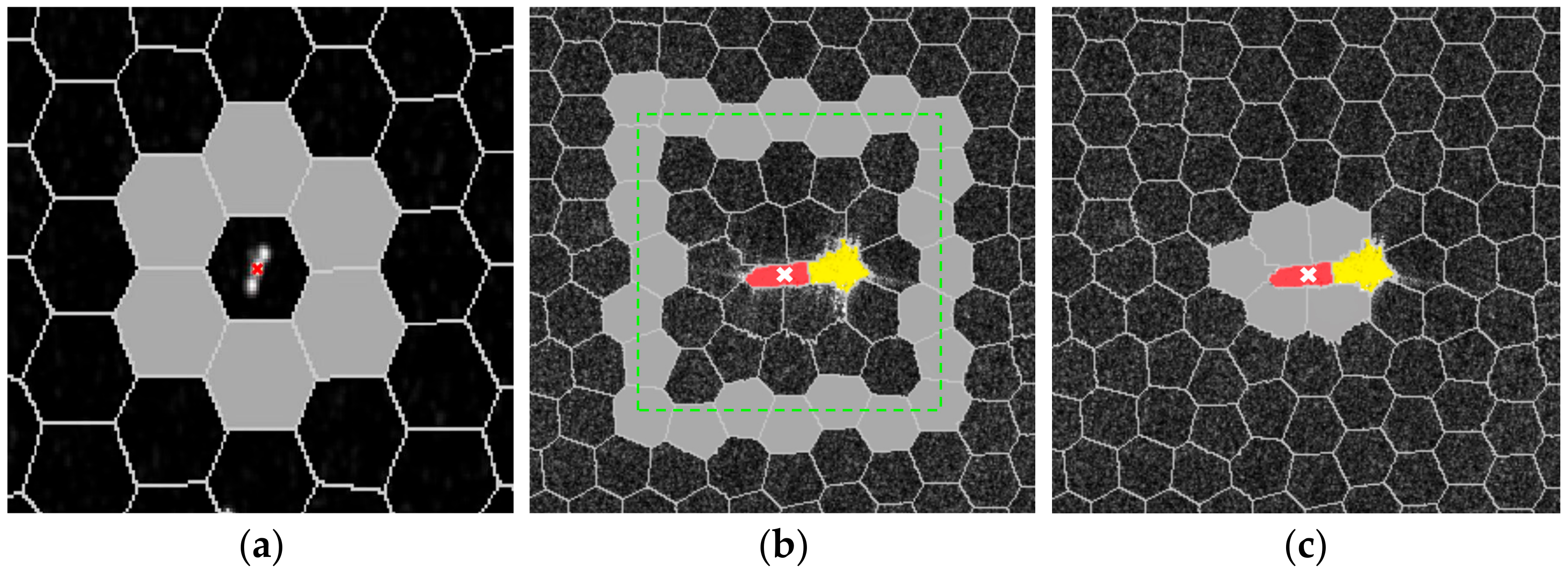
The traditional CFAR algorithm performs pixel-by-pixel detection through a sliding window which contains the clutter area, the guard area and the target area, which has a considerable computational load [10]. Moreover, with the improvement of the SAR image resolution, it would be difficult for the pixel-level CFAR to suppress the false alarms completely while keeping the full shape information of the targets. Superpixels are introduced into the CFAR algorithm which would be beneficial to the selection of clutter area. For the superpixel under test, there are generally three approaches which can obtain the clutter superpixels, as shown in Figure 2. Pappas et al. [6] proposed a topology where the superpixel size is much larger than the ship target to ensure that the ship target is contained in only one superpixel, as shown in Figure 2a. Then, the guard area and the clutter area can be determined accordingly. This method cannot well handle the multiple targets which assemble together. Yu et al. [7] proposed a local sliding window similar to traditional CFAR algorithms, as shown in Figure 2b. Note that this strategy needs the determination of window size according to the target size in SAR images. Moreover, the computation complexity is relatively high. Li et al. [5,35] proposed using a neighborhood strategy to choose the clutter superpixels, as shown in Figure 2c, which illustrates the Bhattacharyya dissimilarity, used to determine the neighbor superpixels. It is worth pointing out that the neighborhood scheme consumes less time to compute clutter statistics with less superpixels. However, the selection accuracy of the clutter superpixels depends on the dissimilarity.

In this subsection, we choose the neighborhood scheme to select the superpixels, which can eliminate the determination of local sliding window size. Moreover, we propose to use the superpixel dissimilarity in Equation (7) to select the pure sea clutter superpixels, making the clutter’s distribution parameter estimation more accurate. Thus, the pixels within one superpixel share the same clutter distribution parameters, which results in a very fast CFAR detection. After the superpixel generation of the SAR image, the superpixel set ${\mathcal{R}}_{all}$ can be obtained. We perform the K-means clustering algorithm to classify the ${\mathcal{R}}_{all}$ into two subsets ${\mathcal{R}}_{target}$ and ${\mathcal{R}}_{background}$ according to the average intensity of each superpixel. The ${\mathcal{R}}_{target}$ contains the superpixels with high intensity values, which may be the ship target and the man-made structures on the land, etc. In contrast, ${\mathcal{R}}_{background}$ is the superpixel set with low intensity values such as the clutter area or the bare soils on the land.

Then, for each under test superpixel $S{P}_i$ in the ${\mathcal{R}}_{target}$, we define an empty set $S_{clutter}$ to contain the clutter superpixels. The local clustering is performed for each neighbor superpixel of $S{P}_i$ which belongs to the ${\mathcal{R}}_{background}$ set. If the dissimilarity measure is more than a predefined threshold $\mathrm{T}{\mathrm{h}}_{clu}$, the neighbor superpixel can be regarded a clutter superpixel and is added into the $S_{clutter}$. We then find all of the neighbor superpixels that in the ${\mathcal{R}}_{background}$ set of the clutter superpixel, then calculate the dissimilarity measures between each neighbor superpixel and the clutter superpixel. The neighbor superpixel whose dissimilarity measures are less than $\mathrm{T}{\mathrm{h}}_{clu}$ can be regarded a new clutter superpixel and is added into the $S_{clutter}$. The iteration procedure will not stop until the termination condition is satisfied, such as the maximum size of $S_{clutter}$. For each superpixel, the neighbor superpixel can be obtained with this manner as follows. For each pixel in the current superpixel, we select its eight neighborhood pixels. If they have the same superpixel label with the test pixel, then move to the next pixel. Otherwise, the neighborhood pixel which has a different superpixel label can be regarded as the pixels in the neighbor superpixel. The pseudocode of the clutter superpixel selection is presented in Algorithm 1, as follows.

Algorithm 1. Clutter Superpixel Selection

Input: the superpixel generation set ${\mathcal{R}}_{all}$ for the SAR image, the threshold $\mathrm{T}{\mathrm{h}}_{clu}$ and the maximum size of $S_{clutter}$.  Output: $S_{clutter}$ for each under test superpixel.  The main steps: 1: Perform the K-means clustering algorithm to classify the ${\mathcal{R}}_{all}$ into two subsets ${\mathcal{R}}_{target}$ and ${\mathcal{R}}_{background}$ according to the average intensity of each superpixel; 2: for each under test superpixel $S{P}_i$ in ${\mathcal{R}}_{target}$ do 3: for each neighbor superpixel $S{P}_i^k$ of $S{P}_i$, $S{P}_i^k\in {\mathcal{R}}_{background}$, do 4: Calculate the superpixel dissimilarity $\mathsf{\Omega }\left(S{P}_i,S{P}_i^k\right)$ 5: The $S{P}_i^k$ with dissimilarity measure more than $\mathrm{T}{\mathrm{h}}_{clu}$ is added into the $S_{clutter}$. 6: end 7: for each neighbor superpixel of the superpixel $S_{clutter}^i$ in $S_{clutter}$ do 8: Calculate the superpixel dissimilarity between $S_{clutter}^i$ and its neighbor superpixel. 9: The neighbor superpixel with dissimilarity measure less than $\mathrm{T}{\mathrm{h}}_{clu}$ is added into the $S_{clutter}$. 10: end 11: Iteratively run step (7) to step (10) until the maximum size of $S_{clutter}$ is achieved. 12: end

The difference between our clutter superpixel selection method and the strategy in Li et al. [5,35] is that our method firstly classify the generated superpixels into the potential target superpixels and background superpixels. Thus the target detection is only performed on the potential target superpixels, which can avoid the calculation for the background superpixels, leading to the acceleration of target detection. Moreover, unlike Figure 2c, our method not only selects the neighbor superpixels of the under test target superpixel, but also can capture the nonlocal superpixels which have the similar attributes with the target superpixel. Therefore, the clutter superpixels can contain more nonlocal information when dealing with the multi-target situation, which contributes to the parameter estimation of the clutter statistical model.

In order to resolve the false alarms such as man-made structures and low bushes, this paper proposes a local superpixel contrast map to enhance the target superpixels. We assume that the ship targets are located in the sea areas, where the superpixels have relatively low intensity values. In contrast, the surrounding areas of man-made structures on the land would have superpixels with relatively higher intensity values. Thus, a local superpixel contrast map can be defined to enhance the local contrast between the ship target superpixels and the background areas, which can optimize the following CFAR detection result. The local contrast value for superpixel $S{P}_m$ can be computed as:

$$C_{local}\left(S{P}_m\right)={\displaystyle \sum }_{S{P}_n\in S_{clutter}}\omega \left(S{P}_m,S{P}_n\right)\mathsf{\Omega }\left(S{P}_m,S{P}_n\right)$$

(9)

where $\mathsf{\Omega }\left(S{P}_m,S{P}_n\right)$ denotes the superpixel dissimilarity. $\omega \left(S{P}_m,S{P}_n\right)$ represents the dissimilarity weight, which can be defined as:

$$\omega \left(S{P}_m,S{P}_n\right)=exp\left(-{\mathrm{D}}_{spatial}\left(S{P}_m,S{P}_n\right)/{\sigma }_{spatial}^2\right)$$

(10)

where ${\mathrm{D}}_{spatial}\left(S{P}_m,S{P}_n\right)$ is the spatial Euclidean distance between the centers of superpixels $S{P}_m$ and $S{P}_n$. ${\sigma }_{spatial}^2$ is a factor and can be set as 0.6 in this paper. From the definition of $C_{local}\left(S{P}_m\right)$, it can be found that the local contrast of superpixel $S{P}_m$ is related to the superpixel dissimilarity and the spatial distance between $S{P}_m$ and its clutter superpixels. For the ship targets in the sea, the dissimilarity measure is large and the spatial distance is low, thus leading to a large contrast. For the man-made structures on the land, although the dissimilarity measure is large, the spatial distance between the man-made structure superpixel and its clutter superpixel is also large, leading to a restively low large contrast. Therefore, the local superpixel contrast map can enhance the significance of potential ship target.

3.4. Superpixel-Based CFAR Detection

After obtaining the clutter superpixels for each potential target superpixel, we can perform the CFAR detection. The gamma distribution is adopted for the clutter statistical model since the gamma distribution is suitable for the high-resolution SAR ship detection. The shape and inverse scale parameter of the gamma distribution can be estimated by using Equation (4), where the pixels used for the estimation are from the clutter superpixels. Thus all the pixels within one under test target superpixel share the same estimated parameters.

Then, for each under test target superpixel $S{P}_m$, the corresponding detection threshold ${\mathrm{Th}}_{cfar}$ can be obtained with a specified false-alarm rate $P_{fa}$ according to the following equation:

$$1-P_{fa}={{\displaystyle \int }}_0^{{\mathrm{Th}}_{cfar}}f\left(x\right)dx$$

(11)

where $f\left(x\right)$ denotes the gamma distribution, as shown in Equation (3). Based on the assumption that the pixels in the same superpixel share similar intensity information, they can be judged using the same threshold since the estimated parameters of the clutter statistical model are the same. Therefore, the decision efficiency can be improved. Based on the following decision criterion, the pixels $I\left(x\right)$ contained in each under test target superpixel $S{P}_m$ can be determined as:

$$\left\{\begin{array}{c}0 \left(background pixels\right) if I\left(x\right)<{\mathrm{Th}}_{cfar}\\ 1 \left(target pixels\right) else if I\left(x\right) \ge {\mathrm{Th}}_{cfar}\end{array}\right.$$

(12)

In order to eliminate the man-made structures false alarms, the local superpixel contrast map $C_{local}\left(S{P}_m\right)$ of superpixel $S{P}_m$ can be considered to optimize the CFAR detection as:

$$\left\{\begin{array}{c}0 \left(background pixels\right) if I\left(x\right)\cdot C_{local}\left(S{P}_m\right)<{\mathrm{Th}}_{cfar}\\ 1 \left(target pixels\right) else if I\left(x\right)·C_{local}\left(S{P}_m\right) \ge {\mathrm{Th}}_{cfar}\end{array}\right.$$

(13)

Due to the man-made structures have relatively low local superpixel contrast values, therefore, the decision in Equation (13) can further suppress the false alarms and enhance the ship target pixels. Finally, the pixel detection result should be mapped to superpixel detection map with post-processing. For the reason that one superpixel contains the pixels with similar attributes, the same superpixel should be labeled as one class. If the number of pixels which are detected as target pixels in Equation (13) exceeds one threshold, the corresponding superpixel should be regarded true target superpixel and all the pixels in it are labeled as target pixels. Otherwise, the superpixel is regarded as background. Thus, the isolated false alarm pixels can be eliminated.

4. Analysis of the Experimental Results

4.1. Data Description

This paper uses four real SAR images for the performance validation. The first dataset is the spaceborne TerraSAR X band SAR data with the image resolution 1-m, as shown in Figure 3a. The imaging area is located in Panama, and the image was acquired in January 2014 using spotlight mode. The image size is $1542\times 1506$, and the polarization mode is HH. The sea condition is low. The second SAR image is also TerraSAR data with 1-m resolution. The polarization mode is a VV with spotlight mode. The image size is $1069\times 695$, as shown in Figure 3b. The imaging area is located in Visakhapatnam, and the imaging date is October 2008. The sea condition is low.

The third SAR image is Gaofen 3 (GF-3) C band data with the image size $1295\times 1200$. The polarization mode is HH. The resolution is 1 m in azimuth direction and 1.5 m in range direction, as shown in Figure 3c. The sea condition is middle, i.e., 4 level. The fourth SAR image is acquired by the Sentinel-1A sensor with C band using IW mode, where the image size is $765\times 807$ and the resolution is 20 m. The imaging area is located in the Guangdong-Hong Kong-Macao Greater Bay Area, China and the image date is January 2021. The sea condition is 2 level.

Figure 4 gives the corresponding ground truth, which indicates the true ship pixels. Note that due to the lack of automatic identification system information, the ground truth is obtained with photointerpretation by comparing with the Google map reference and expert manually marking. It is worth pointing out that in Figure 3c there are some ships with different sizes. It is used for the validation of our method on the performance of multi-scale ship detection.

4.2. Ship Detection Results of the Proposed Method

Figure 5 shows the results of the first TerraSAR X band SAR image with our proposed method. The superpixel segmentation result is given in Figure 5a, where the superpixel number is 8000. It can be seen that the DBSCAN superpixel generation method can produce fine superpixels which can adhere well to the image boundaries and preserve the ship targets. Figure 5b shows the target superpixels of the proposed method, where it can be seen that superpixels with high image contrast and intensity are selected for the following CFAR detection. Thus the detection procedure can be more efficient than the traditional CFAR detector for the reason that not all the pixels are tested in our method.

Figure 5c presents the local superpixel contrast map, indicating the superpixels with relatively high local contrast. It can be seen that the ships have high contrast whereas the land areas have relatively low contrast, which can be beneficial to the false alarm removal. Figure 5d gives the final ship detection result for the TerraSAR image, where we can see that the details of the ships can be well preserved and the forests on the land are removed although there also exists high backscattering.

The detection results of the second TerraSAR image by using our method is given in Figure 6, where the superpixel number is set as 6500. It can be seen that there are urban buildings and forests on the land, which would easily lead to false alarms for ship detection. The buildings and forests with relatively high backscattering are selected as target superpixels in Figure 6b. However, our detection result map can remove the false alarms thanks to the local superpixel contrast map, as shown in Figure 6c,d.

Figure 7 presents the ship detection results of the GF-3 C band image, where there exist multiple targets with different sizes. Moreover, the sea state condition is relatively high. The superpixel number is set as 8000. It can be found that the target superpixels in Figure 7b have high backscattering. Most of the background areas are determined and removed for the following ship detection, including the clutter background with high sea state. With the consideration of local superpixel contrast, the ship detection result in Figure 7d is satisfactory. Figure 8 shows the results of Sentinel-1A C band SAR image, where we can see that there are some large and small ships, as well as some man-made structures in the sea. The superpixel number is set as 6000. In Figure 8b, we can find that the man-made structures are eliminated with the target superpixel identification procedure. In the local superpixel contrast map, the false alarms on the island are suppressed, leading to a satisfactory ship detection result in Figure 8d. It is worth pointing out that the small ships can be well preserved, indicating that our method can effectively extract ships with multi-scale sizes.

4.3. The Performance Discussion on the Parameters of the Proposed Method

The parameters involved in our method include the number of generation superpixels, the threshold $T_{sh}$ for shadow superpixel removal, the threshold $\mathrm{T}{\mathrm{h}}_{clu}$ for clutter superpixel selection, the maximum size of $S_{clutter}$ and the number of target pixels in a superpixel for post-processing. As we stated before, the shadow superpixel threshold $T_{sh}$ can be set according to the average pixel intensity of the shadow regions in the training data, which is easily determined. The maximum size of $S_{clutter}$ can influence the estimation accuracy of clutter model parameters. Larger size of $S_{clutter}$ would make the estimation more accurate with more samples. However, the efficiency would also be decreased. In general, we set the maximum size of $S_{clutter}$ as 8 since enough pixel samples can be obtained for the estimation with the consideration of computation complexity. In the post-processing, the number of target pixels in a superpixel would influence the final detection map. In generally, we can set a ratio, that is, the number of target pixels divided by the total number of pixels in the superpixel as a threshold for the post-processing. Experimental results indicate that 0.7 would be fine for most of the images.

In terms of the threshold $\mathrm{T}{\mathrm{h}}_{clu}$ for clutter superpixel selection, we think it is related to the superpixel size and average intensity according to Equations (7) and (8). Therefore, this parameter should be determined according to the SAR image scenes. In the experiments, we select some training areas to calculate the threshold $\mathrm{T}{\mathrm{h}}_{clu}$.

The final parameter should be discussed is the superpixel number, which also has a great influence on the ship detection. In general, more superpixels would obtain more segments, leading to a better preservation ability of the ship target details. However, there are some drawbacks. On one hand, the computation load of ship detection will increase with the number of superpixels since more parameter estimation and CFAR detection should be performed. On the other hand, there will exist over-segmentation errors with more superpixels for one target, thus resulting in some omissions.

In order to quantitatively evaluate the performance of the ship target detection results, this paper adopts $FAR$ (false alarm rate) and $ADR$ (actual detection rate) as quantitative evaluation indicators, which are defined as follows [5,6,13]:

$$FAR=\frac{N_{dc}}{N_C}$$

(14)

$$ADR=\frac{N_{dt}}{N_T}$$

(15)

where $N_C$ and $N_T$ represent the total number of clutter pixels and target pixels, respectively. $N_{dt}$ and $N_{dc}$ denote the number of correctly detected target pixels and those of the false-alarm pixels. The smaller the $FAR$, the lower the false alarm rate of the detection result. The higher the $ADR$, the higher the accuracy of the detection result. In order to validate the performance of superpixel number on the final ship detection result, we select the first TerraSAR image to obtain four superpixel segmentation results with the superpixel number as 4000, 6000, 8000, 10,000. Then, we perform the ship detection using our method and calculate the $FAR$ and $ADR$ measures of the detection results, as shown in

Table 1. Quantitative measures of our proposed method with different superpixel number.

	The Superpixel Number
	4000		6000		8000		10,000
	FAR(%)	ADR(%)	FAR(%)	ADR(%)	FAR(%)	ADR(%)	FAR(%)	ADR(%)
The first TerraSAR data	0.37	82.4	0.39	86.5	0.35	88.2	0.42	87.9

.

With the increasing of superpixel number from 4000 to 8000, the $ADR$ becomes higher and the $FAR$ becomes lower. The best result can be achieved when the number is 8000. However, if we increase the superpixel number to 10,000, the $ADR$ achieves steady whereas the $FAR$ becomes slightly worse. The reason is that some over-segmentation errors exist and leads some omissions and false alarms. More importantly, the computation load becomes higher with the increasing of superpixel number, which will be depicted in the next subsection.

5. Discussions

5.1. Comparison Analysis among Different Methods

In order to further verify the effectiveness of the proposed method, the conventional two-parameter CFAR detection method, SP-CFAR method [6], and superpixel-level CFAR detector, based on truncated gamma distribution (SP-CFAR-TG) [5], were used as comparison methods. The size of the sliding window of traditional two-parameter CFAR was selected based on the user’s experience according to the information of different images. The parameters in the SP-CFAR method and SP-CFAR-TG method were set according to the references. For fairness, the superpixel segmentation results were kept the same as that for our method. The ship detection results of four SAR datasets with three methods are shown in Figure 9, Figure 10, Figure 11 and Figure 12.

We can see from the detection results that the conventional two-parameter CFAR detection method cannot accurately capture the target details and eliminate false alarms for the reason that this method belongs to the pixel-by-pixel detection strategy. Therefore, the detected targets consist of fractures and holes. Moreover, many false alarm pixels appear in the land region. This result indicates that only the consideration of pixel intensity value for ship detection is sensitive to speckle noise, the existence of man-made structures, and forests that have relatively high backscattering. Moreover, this method is quite sensitive to the local sliding window size, which should be set according to the image resolution and the target size. As CFAR target detection algorithms based on superpixels, SP-CFAR and SP-CFAR-TG can effectively maintain the target pixels and details. This is because the superpixel segmentation can effectively preserve the image of the shiptarget details and shapes.

However, there is a situation of missed detection and false alarms in dense ship targets and inshore ship images. The reason for this is that some superpixels with assembled high backscattering pixels could be regarded as ship targets. In our method, clutter superpixels are selected by using an iterative manner, which can more accurately estimate the clutter model parameters. Moreover, we use the local superpixel contrast map to suppress the false alarms on the land. Therefore, our method can achieve better ship detection results in comparison with other three approaches.

Table 2. Quantitative comparisons of four target detection algorithms with four SAR datasets.

	Two-Parameter CFAR		SP-CFAR		SP-CFAR-TG		The Proposed Method
	FAR(%)	ADR(%)	FAR(%)	ADR(%)	FAR(%)	ADR(%)	FAR(%)	ADR(%)
The first TerraSAR data	2.75	77.1	1.68	81.1	0.87	84.6	0.35	88.2
The second TerraSAR data	3.54	72.3	1.85	80.5	0.98	83.4	0.47	86.7
GF-3 data	2.22	76.5	1.92	74.2	0.76	84.5	0.66	92.8
Sentinel-1A data	1.25	81.5	0.83	86.5	0.71	93.4	0.70	98.4

shows the quantitative measures of different methods for the SAR datasets. The false alarm rate of the conventional two-parameter CFAR detector is much higher than the other methods, especially for the high-resolution TerraSAR data and GF-3 data with a middle sea level condition. This is because this method cannot handle the clutter false alarms on land. For the Sentinel-1A SAR data, the false alarm rate decreases as the image scenes are not complex. In the evaluation results of SP-CFAR and SP-CFAR-TG, there are still some false alarms for the high-resolution TerraSAR data, indicating that the false removal of land structures and forests is a challenging problem. In contrast, our method can obtain satisfactory results due to the local superpixel contrast map and accurate clutter selection procedures.

5.2. The Computational Complexity Analysis

As we discussed in the previous sections, the superpixel-based CFAR detectors can accelerate the conventional CFAR detection for the reason that the number of superpixels is dramatically less than the number of pixels. This subsection gives the time costs comparison of different methods for the SAR datasets, as shown in

Table 3. Time costs of four ship detection algorithms for different SAR images.

	Two-Parameter CFAR	SP-CFAR	SP-CFAR-TG	The Proposed Method
	Time (Second)	Time (Second)	Time (Second)	Time (Second)
The first TerraSAR data	1669.22	383.96	240.66	47.56
The second TerraSAR data	365.39	164.28	125.39	40.45
GF-3 data	929.87	263.17	196.45	43.98
Sentinel-1A data	225.37	110.82	93.57	29.69

. Moreover, for our method, the detection efficiency with different superpixel numbers is also discussed. Note that the superpixel generation procedure belongs to the pre-processing stage, and the time costs of superpixel segmentation are the same for the SP-CFAR, SP-CFAR-TG, and the proposed method in this experiment for the reason that they use the same superpixel generation method. All the experimental results are conducted with the Matlab language. It can be seen that the conventional two-parameter CFAR detector has much higher time costs than other methods for the four SAR datasets. In contrast, the SP-CFAR and the SP-CFAR-TG methods significantly reduce the time costs thanks to the introduction of superpixels. However, our method still has a much lower time cost than the two methods. The reason is that we only perform the CFAR detection on target superpixels, which can speed up the detection procedure. In order to further discuss the time costs of our method with different numbers of superpixels, we give

Table 4. Time costs of our method for the first TerraSAR data with different superpixel numbers.

	The Superpixel Number
	4000	6000	8000	10,000
	Time (Second)	Time (Second)	Time (Second)	Time (Second)
The first TerraSAR data	33.68	41.37	47.56	65.84

. It can be seen that when the superpixel number changes from 8000 to 10,000, the computation load has a large increment, which can indicate the statement that not more superpixels would lead to better detection results.

5.3. Limitations of the Proposed Method

From the analysis of the above results, we find that the superpixel generation result and the local superpixel contrast map have a great influence on ship detection in our proposed method. Actually, superpixels with good boundary adherence and compactness could accurately preserve ship details, thus leading to a satisfactory ship detection result. More importantly, satisfactory superpixels are also beneficial for the calculation of local superpixel contrast map, which can also contribute to false alarm reduction. In our proposed method, we adopted our previously proposed superpixel generation approach, i.e., a DBSCAN strategy for the SAR image superpixel generation. However, the edge constraint in the DBSCAN method is not considered due to its efficiency. Therefore, more efficient superpixel generation methods with a good boundary adherence and compactness would increase the performance of the proposed ship detection method.

6. Conclusions

In order to improve the robustness of CFAR to the speckle noise in SAR images and the detection efficiency, this paper proposes a new superpixel-based CFAR ship detection method for SAR images, which introduces the superpixels to CFAR detection. Our previously proposed fast DBSCAN superpixel generation method is utilized to produce the superpixels for SAR images. Then, the superpixel dissimilarity is defined to accurately estimate the clutter parameters for the under test pixel, even in the multi-target situations, avoiding the drawbacks of sliding window in the traditional CFAR. Moreover, a local superpixel contrast is proposed to optimize the CFAR detection, which can eliminate the numerous clutter false alarms. The proposed CFAR detection can better preserve the ship target shape and details with less false alarms in comparison with other state-of-the-art superpixel based CFAR detectors. Future work will focus on the optimization of a local superpixel contrast map, leading to a better performance for false alarm reduction.

References

1. Weiss, M. Analysis of some modified cell-averaging CFAR processors in multiple-target situations. IEEE Trans. Aerosp. Electron. Syst. 1982, 18, 102–114. [Google Scholar] [CrossRef]
2. Barkat, M.; Himonas, S.; Varshney, P. CFAR detection for multiple target situations. IEE Proc. F Radar Signal Process. 1989, 136, 193–209. [Google Scholar] [CrossRef]
3. Busch, S.; Lehner, S.; Fritz, T.; Soccorsi, M.; Soloviev, A.; van Schie, B. Ship surveillance with TerraSAR-X. IEEE Trans. Geosci. Remote Sens. 2010, 49, 1092–1103. [Google Scholar] [CrossRef]
4. Novak, L.; Hesse, S. On the Performance of Order-Statistics CFAR Detectors. In Proceedings of the Conference Record of the Twenty-Fifth Asilomar Conference on Signals, Systems & Computers, Pacific Grove, CA, USA, 4–6 November 1991; pp. 835–840. [Google Scholar]
5. Li, T.; Peng, D.; Chen, Z.; Guo, B. Superpixel-level CFAR detector based on truncated gamma distribution for SAR images. IEEE Geosci. Remote Sens. Lett. 2020, 18, 1421–1425. [Google Scholar] [CrossRef]
6. Pappas, O.; Achim, A.; Bull, D. Superpixel-level CFAR detectors for ship detection in SAR imagery. IEEE Geosci. Remote Sens. Lett. 2018, 15, 1397–1401. [Google Scholar] [CrossRef] [Green Version]
7. Yu, W.; Wang, Y.; Liu, H.; He, J. Superpixel-based CFAR target detection for high-resolution SAR images. IEEE Geosci. Remote Sens. Lett. 2016, 13, 730–734. [Google Scholar] [CrossRef]
8. Cui, Y.; Zhou, G.; Yang, J.; Yamaguchi, Y. On the iterative censoring for target detection in SAR images. IEEE Geosci. Remote Sens. Lett. 2011, 8, 641–645. [Google Scholar] [CrossRef]
9. An, W.; Xie, C.; Yuan, X. An improved iterative censoring scheme for CFAR ship detection with SAR imagery. IEEE Trans. Geosci. Remote Sens. 2013, 52, 4585–4595. [Google Scholar]
10. Gao, G.; Liu, L.; Zhao, L.; Shi, G.; Kuang, G. An adaptive and fast CFAR algorithm based on automatic censoring for target detection in high-resolution SAR images. IEEE Trans. Geosci. Remote Sens. 2008, 47, 1685–1697. [Google Scholar] [CrossRef]
11. Hou, B.; Chen, X.; Jiao, L. Multilayer CFAR detection of ship targets in very high resolution SAR images. IEEE Geosci. Remote Sens. Lett. 2014, 12, 811–815. [Google Scholar]
12. Leng, X.; Ji, K.; Yang, K.; Zou, H. A bilateral CFAR algorithm for ship detection in SAR images. IEEE Geosci. Remote Sens. Lett. 2015, 12, 1536–1540. [Google Scholar] [CrossRef]
13. Li, T.; Liu, Z.; Xie, R.; Ran, L. An improved superpixel-level CFAR detection method for ship targets in high-resolution SAR images. IEEE J. Sel. Top. Appl. Earth Observ. Remote Sens. 2017, 11, 184–194. [Google Scholar] [CrossRef]
14. Wang, Z.; Du, L.; Su, H. Target detection via Bayesian-morphological saliency in high-resolution SAR images. IEEE Trans. Geosci. Remote Sens. 2017, 55, 5455–5466. [Google Scholar] [CrossRef]
15. Xiang, D.; Tang, T.; Zhao, L.; Su, Y. Superpixel generating algorithm based on pixel intensity and location similarity for SAR image classification. IEEE Geosci. Remote Sens. Lett. 2013, 10, 1414–1418. [Google Scholar] [CrossRef]
16. Zhang, W.; Xiang, D.; Su, Y. Fast multiscale superpixel segmentation for SAR imagery. IEEE Geosci. Remote Sens. Lett. 2020, 19, 4001805. [Google Scholar] [CrossRef]
17. Liu, M.; Chen, S.; Lu, F.; Xing, M.; Wei, J. Realizing Target Detection in SAR Images Based on Multiscale Superpixel Fusion. Sensors 2021, 21, 1643. [Google Scholar] [CrossRef]
18. Li, M.-D.; Cui, X.-C.; Chen, S.-W. Adaptive superpixel-level CFAR detector for SAR inshore dense ship detection. IEEE Geosci. Remote Sens. Lett. 2021, 19, 1–5. [Google Scholar] [CrossRef]
19. Guo, H.; Yang, X.; Wang, N.; Gao, X.J. A CenterNet++ model for ship detection in SAR images. Pattern Recognit. 2021, 112, 107787. [Google Scholar] [CrossRef]
20. Li, D.; Liang, Q.; Liu, H.; Liu, Q.; Liu, H.; Liao, G. A novel multidimensional domain deep learning network for SAR ship detection. IEEE Trans. Geosci. Remote Sens. 2021, 60, 1–13. [Google Scholar] [CrossRef]
21. Zhang, T.; Zhang, X.J. High-speed ship detection in SAR images based on a grid convolutional neural network. Remote Sens. 2019, 11, 1206. [Google Scholar] [CrossRef] [Green Version]
22. Wang, Y.; Wang, C.; Zhang, H.; Dong, Y.; Wei, S.J. Automatic ship detection based on RetinaNet using multi-resolution Gaofen-3 imagery. Remote Sens. 2019, 11, 531. [Google Scholar] [CrossRef] [Green Version]
23. Zhang, T.; Zhang, X.; Shi, J.; Wei, S.J. Depthwise separable convolution neural network for high-speed SAR ship detection. Remote Sens. 2019, 11, 2483. [Google Scholar] [CrossRef] [Green Version]
24. Li, J.; Qu, C.; Shao, J. Ship detection in SAR images based on an improved faster R-CNN. In Proceedings of the 2017 SAR in Big Data Era: Models, Methods and Applications (BIGSARDATA), Beijing, China, 13–14 November 2017; pp. 1–6. [Google Scholar]
25. Huang, L.; Liu, B.; Li, B.; Guo, W.; Yu, W.; Zhang, Z.; Yu, W. OpenSARShip: A dataset dedicated to Sentinel-1 ship interpretation. IEEE J. Sel. Top. Appl. Earth Observ. Remote Sens. 2017, 11, 195–208. [Google Scholar] [CrossRef]
26. Zhang, L.; Lu, S.; Hu, C.; Xiang, D.; Liu, T.; Su, Y. Superpixel Generation for SAR Imagery Based on Fast DBSCAN Clustering with Edge Penalty. IEEE J. Sel. Top. Appl. Earth Observ. Remote Sens. 2021, 15, 804–819. [Google Scholar] [CrossRef]
27. Kuruoglu, E.E.; Zerubia, J. Modeling SAR images with a generalization of the Rayleigh distribution. IEEE Trans. Image Process. 2004, 13, 527–533. [Google Scholar] [CrossRef] [PubMed]
28. Nar, F.; Okman, O.E.; Özgür, A.; Çetin, M. Fast target detection in radar images using Rayleigh mixtures and summed area tables. Digit. Signal Process. 2018, 77, 86–101. [Google Scholar] [CrossRef]
29. Li, H.-C.; Krylov, V.A.; Fan, P.-Z.; Zerubia, J.; Emery, W.J. Unsupervised learning of generalized gamma mixture model with application in statistical modeling of high-resolution SAR images. IEEE Trans. Geosci. Remote Sens. 2015, 54, 2153–2170. [Google Scholar] [CrossRef] [Green Version]
30. Rodrigues, F.Á.; Neto, J.R.; Marques, R.P.; de Medeiros, F.S.; Nobre, J.S. SAR image segmentation using the roughness information. IEEE Geosci. Remote Sens. Lett. 2016, 13, 132–136. [Google Scholar] [CrossRef]
31. Achanta, R.; Shaji, A.; Smith, K.; Lucchi, A.; Fua, P.; Süsstrunk, S.J. SLIC superpixels compared to state-of-the-art superpixel methods. IEEE Trans. Pattern Anal. Mach. Intell. 2012, 34, 2274–2282. [Google Scholar] [CrossRef] [Green Version]
32. Jing, W.; Jin, T.; Xiang, D. Content-Sensitive Superpixel Generation for SAR Images with Edge Penalty and Contraction–Expansion Search Strategy. IEEE Trans. Geosci. Remote Sens. 2021, 60, 1–15. [Google Scholar] [CrossRef]
33. Jing, W.; Jin, T.; Xiang, D. Edge-aware superpixel generation for SAR imagery with one iteration merging. IEEE Geosci. Remote Sens. Lett. 2020, 18, 1600–1604. [Google Scholar] [CrossRef]
34. Xiang, D.; Tang, T.; Quan, S.; Guan, D.; Su, Y. Adaptive superpixel generation for SAR images with linear feature clustering and edge constraint. IEEE Trans. Geosci. Remote Sens. 2019, 57, 3873–3889. [Google Scholar] [CrossRef]
35. Li, T.; Liu, Z.; Ran, L.; Xie, R. Target detection by exploiting superpixel-level statistical dissimilarity for SAR imagery. IEEE Geosci. Remote Sens. Lett. 2018, 15, 562–566. [Google Scholar] [CrossRef]
Figure 1. Flowchart of the proposed SP-NW-CFAR detection method.
Remotesensing 14 02092 g001
Figure 2. Strategies for the clutter superpixels determination (shown in gray) for the current test superpixels (marked with red). (a) The superpixel is much larger than the ship target. (b) Local sliding window around the test superpixel. (c) Neighborhood determination around the test superpixel.
Remotesensing 14 02092 g002
Figure 3. The SAR datasets with different bands and resolutions. (a) The first TerraSAR X band SAR image. (b) The second TerraSAR X band SAR image. (c) GF-3 C band SAR image. (d) Sentinel-1A C band SAR image.
Remotesensing 14 02092 g003aRemotesensing 14 02092 g003b
Figure 4. The ground truth map of the SAR images. (a) The first TerraSAR X band SAR image. (b) The second TerraSAR X band SAR image. (c) GF-3 C band SAR image. (d) Sentinel-1A C band SAR image.
Remotesensing 14 02092 g004aRemotesensing 14 02092 g004b
Figure 5. The results of the first TerraSAR X band SAR image with our proposed method. (a) The superpixel segmentation result. (b) The target superpixel map. (c) The local superpixel contrast map. (d) Final ship detection result.
Remotesensing 14 02092 g005
Figure 6. The results of the second TerraSAR X band SAR image with our proposed method. (a) The superpixel segmentation result. (b) The target superpixel map. (c) The local superpixel contrast map. (d) Final ship detection result.
Remotesensing 14 02092 g006
Figure 7. The results of the GF-3 C band SAR image with our proposed method. (a) The superpixel segmentation result. (b) The target superpixel map. (c) The local superpixel contrast map. (d) Final ship detection result.
Remotesensing 14 02092 g007
Figure 8. The results of the Sentinel-1A C band SAR image with our proposed method. (a) The superpixel segmentation result. (b) The target superpixel map. (c) The local superpixel contrast map. (d) Final ship detection result.
Remotesensing 14 02092 g008aRemotesensing 14 02092 g008b
Figure 9. The detection results of the first TerraSAR SAR image with three compared methods. (a) The result of two-parameter CFAR. (b) The result of SP-CFAR. (c) The result of SP-CFAR-TG.
Remotesensing 14 02092 g009
Figure 10. The detection results of the second TerraSAR SAR image with three compared methods. (a) The result of two-parameter CFAR. (b) The result of SP-CFAR. (c) The result of SP-CFAR-TG.
Remotesensing 14 02092 g010
Figure 11. The detection results of the GF-3 SAR image with three compared methods. (a) The result of two-parameter CFAR. (b) The result of SP-CFAR. (c) The result of SP-CFAR-TG.
Remotesensing 14 02092 g011
Figure 12. The detection results of the Sentinel-1A SAR image with three compared methods. (a) The result of two-parameter CFAR. (b) The result of SP-CFAR. (c) The result of SP-CFAR-TG.
Remotesensing 14 02092 g012