
The Potential of 3-D Building Height Data to Characterize Socioeconomic Activities: A Case Study from 38 Cities in China


 ,
,  and
and 
Abstract
:1. Introduction
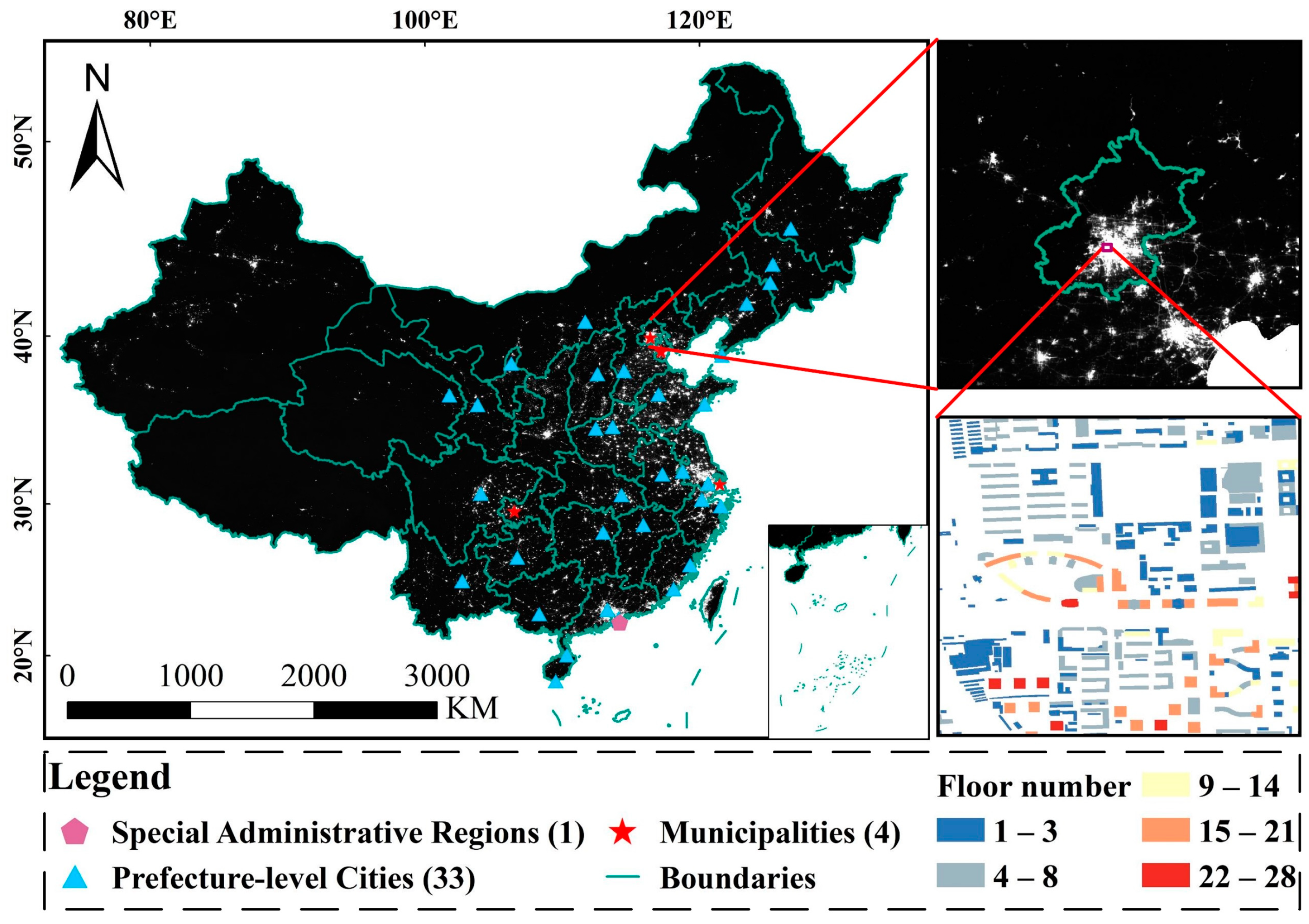
2. Materials
3. Methodologies
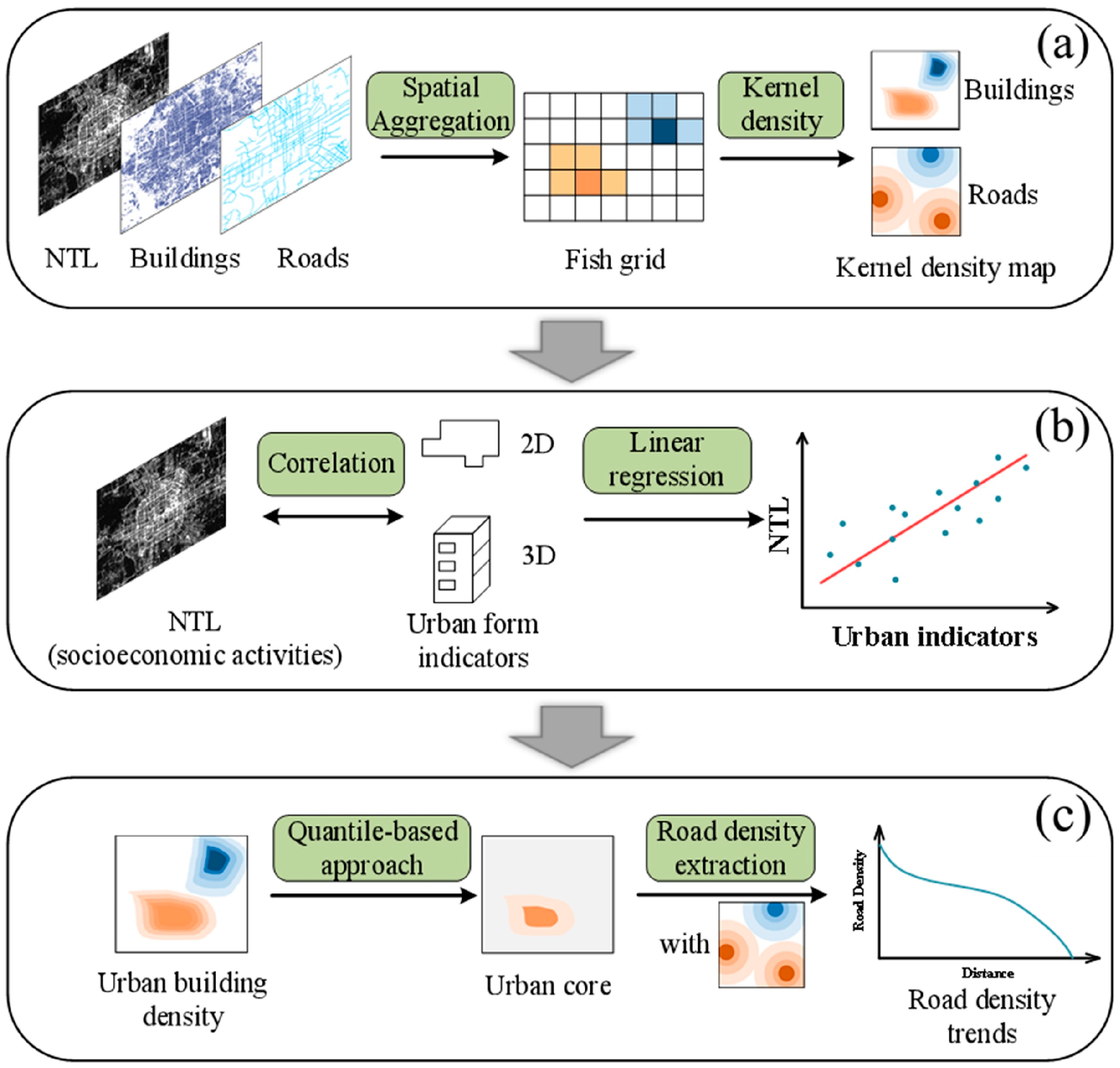
3.1. Data Preprocess
3.2. The Correlation between Urban Form and NTL
3.3. The Relationship between Road Density and Building Height
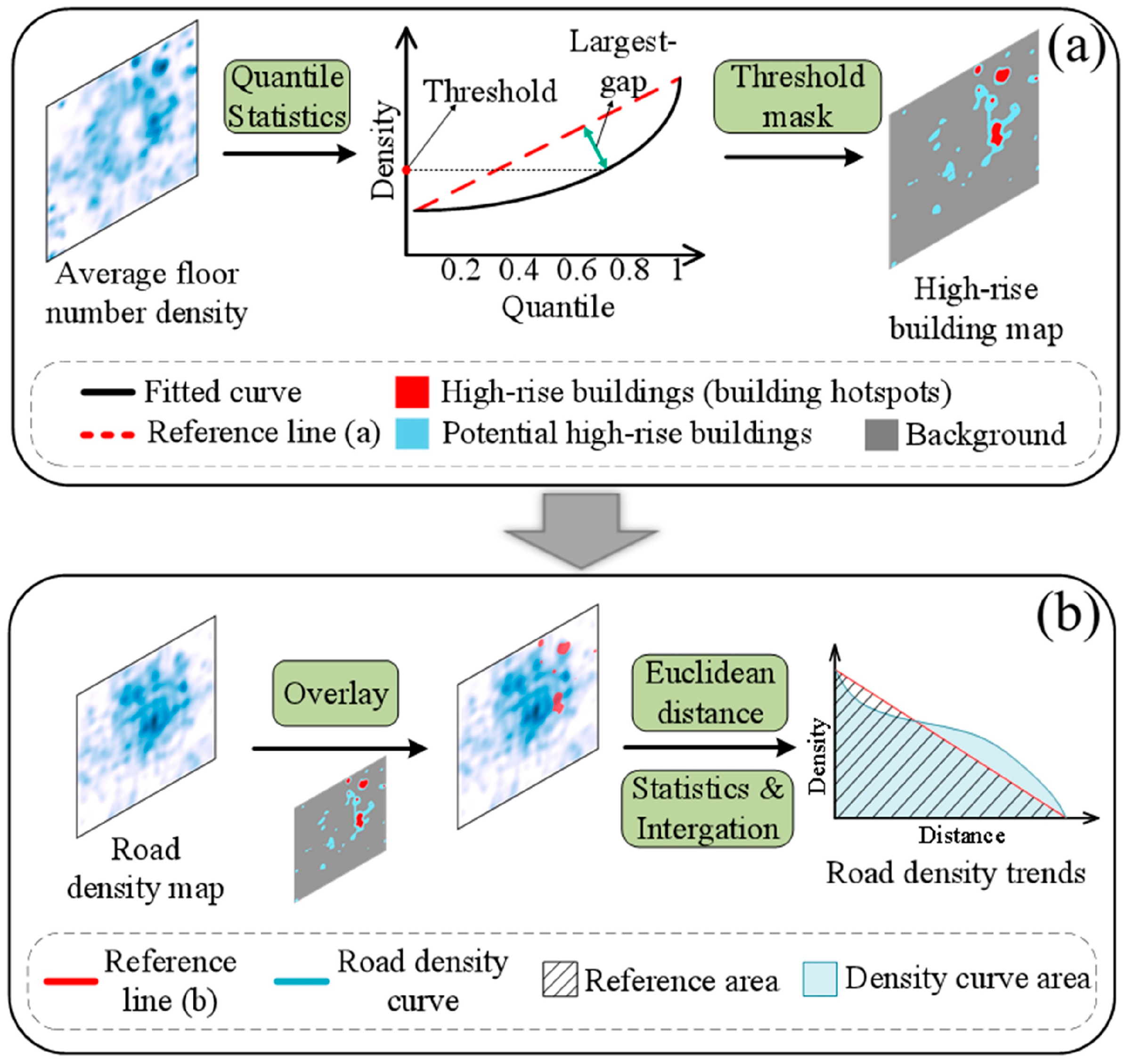
3.3.1. Quantile-Based Approach to Building Masking
3.3.2. Road Distribution Pattern Extraction
4. Results and Discussion
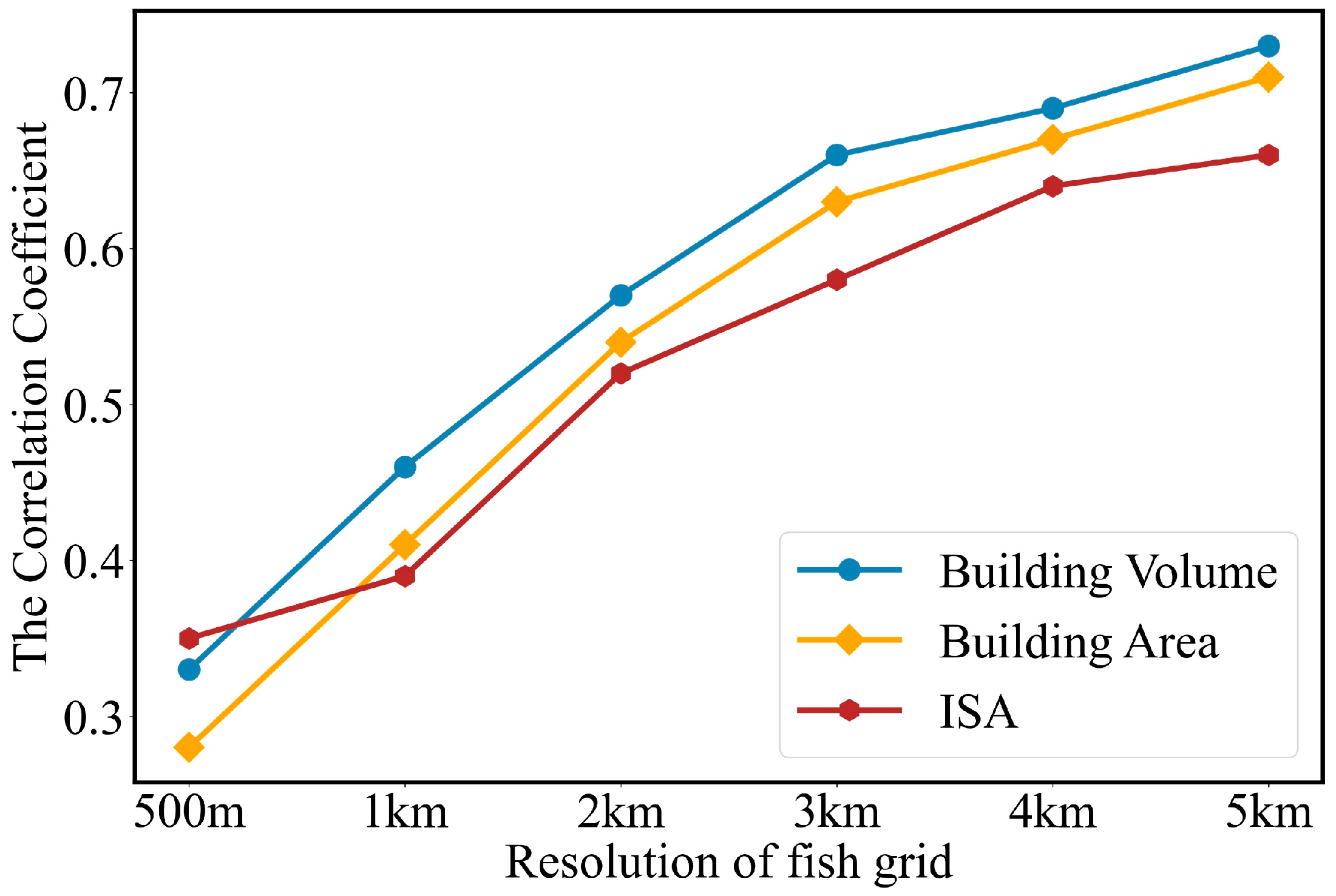
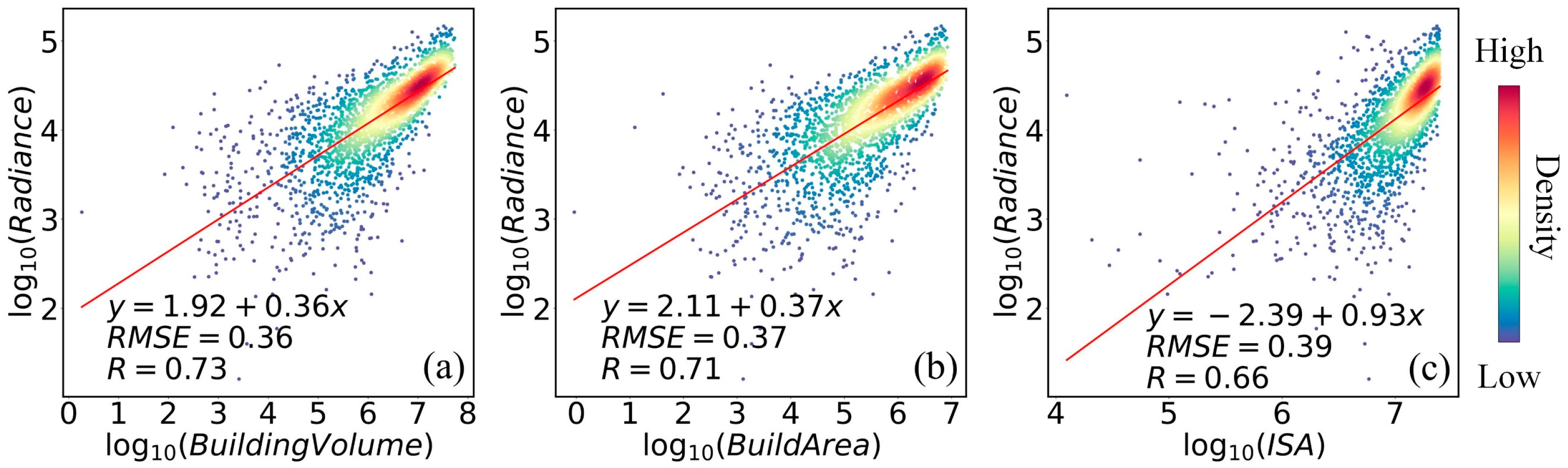
4.1. Correlation with NTL Data
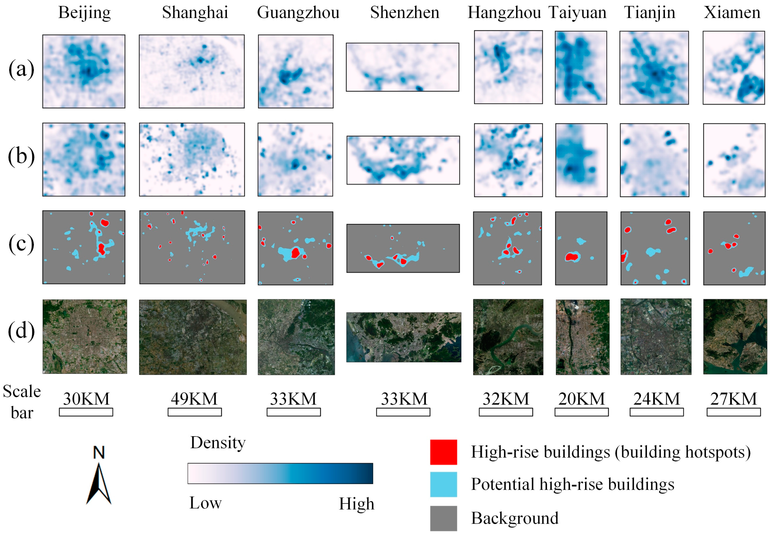
4.2. The Extracted Urban Cores
4.3. Identification of Road Distribution Patterns
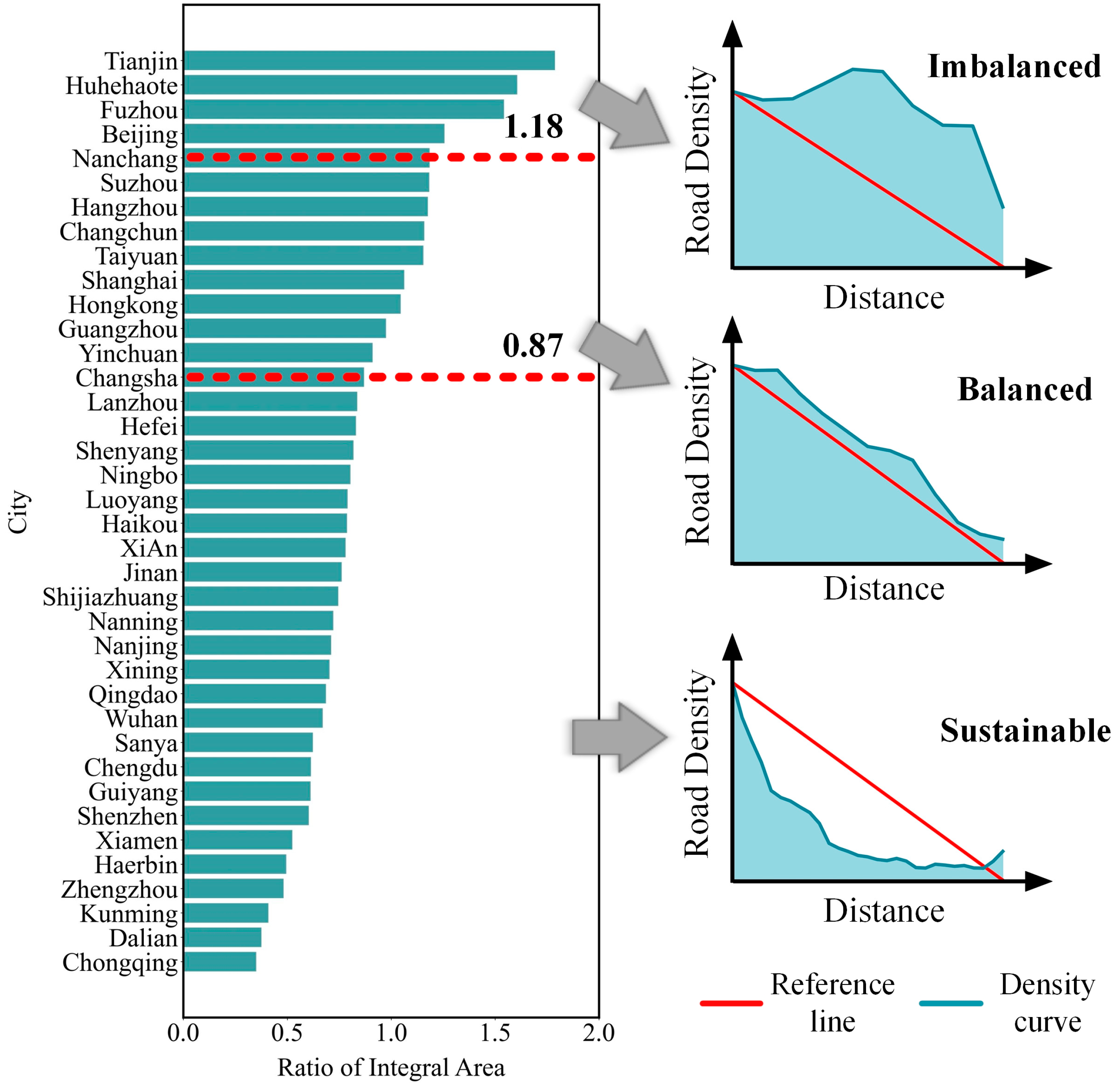
4.3.1. Classification of Road Distribution Patterns
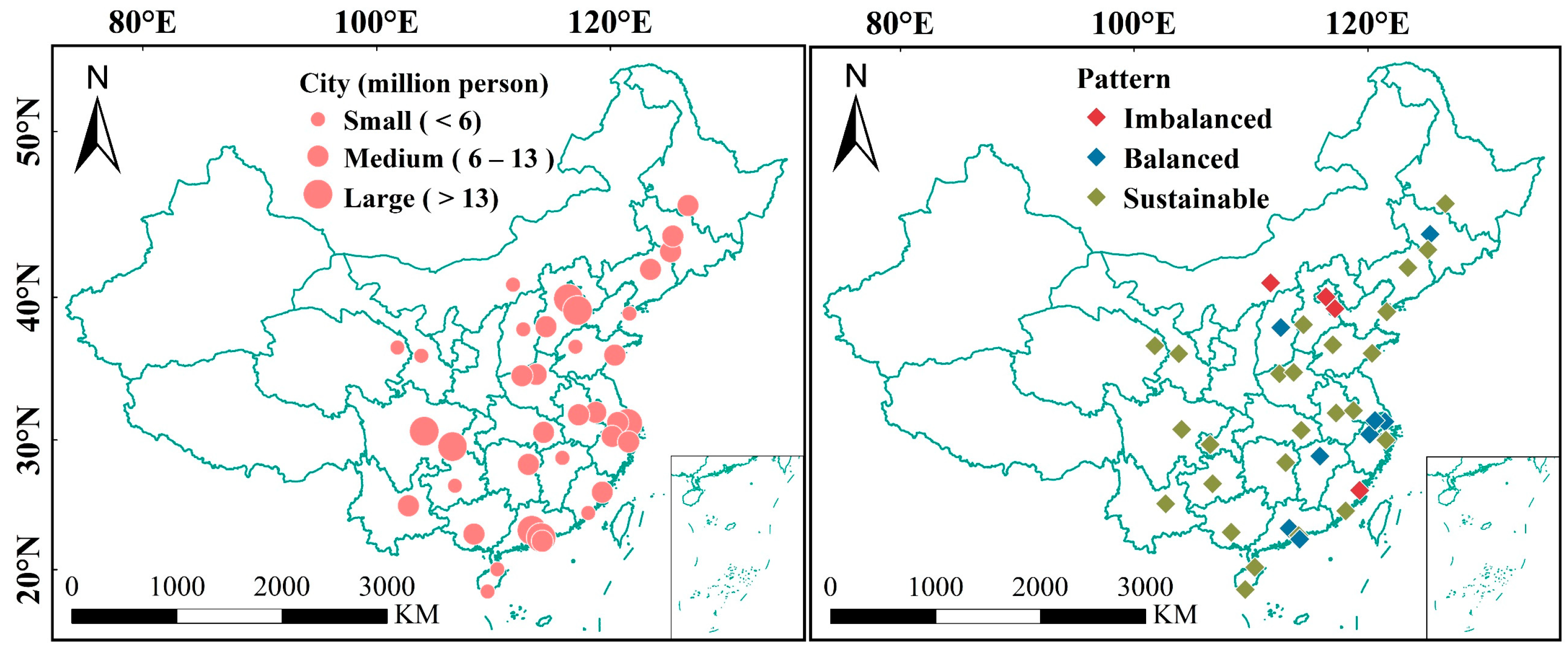
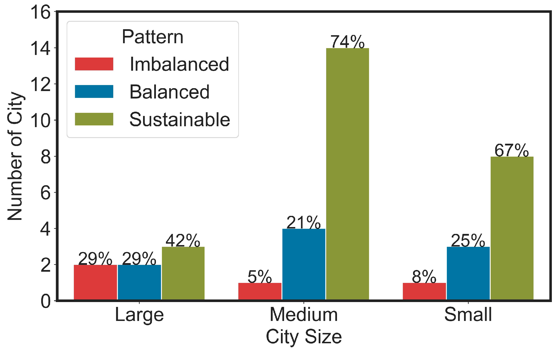
4.3.2. Association with City Size
4.3.3. Differences among Road Distribution Patterns
5. Conclusions
Supplementary Materials
Author Contributions
Funding
Data Availability Statement
Acknowledgments
Conflicts of Interest
References
- Cohen, B. Urbanization in developing countries: Current trends, future projections, and key challenges for sustainability. Technol. Soc. 2006, 28, 63–80. [Google Scholar] [CrossRef]
- Chen, J. Rapid urbanization in China: A real challenge to soil protection and food security. Catena 2007, 69, 1–15. [Google Scholar] [CrossRef]
- Arfanuzzaman, M.; Dahiya, B. Sustainable urbanization in Southeast Asia and beyond: Challenges of population growth, land use change, and environmental health. Growth Chang. 2019, 50, 725–744. [Google Scholar] [CrossRef]
- Xiong, Y.; Huang, S.; Chen, F.; Ye, H.; Wang, C.; Zhu, C. The Impacts of Rapid Urbanization on the Thermal Environment: A Remote Sensing Study of Guangzhou, South China. Remote Sens. 2012, 4, 2033–2056. [Google Scholar] [CrossRef] [Green Version]
- United Nations, Department of Economic and Social Affairs. World Urbanization Prospects: The 2018 Revision (ST/ESA/SER.A/420); United Nations, Department of Economic and Social Affairs: New York, NY, USA, 2019; Volume 12, ISBN 9789211483192. [Google Scholar]
- Dadashpoor, H.; Azizi, P.; Moghadasi, M. Land use change, urbanization, and change in landscape pattern in a metropolitan area. Sci. Total Environ. 2019, 655, 707–719. [Google Scholar] [CrossRef] [PubMed]
- Wu, H.; Lin, A.; Xing, X.; Song, D.; Li, Y. Identifying core driving factors of urban land use change from global land cover products and POI data using the random forest method. Int. J. Appl. Earth Obs. Geoinf. 2021, 103, 102475. [Google Scholar] [CrossRef]
- Yin, C.; Yuan, M.; Lu, Y.; Huang, Y.; Liu, Y. Effects of urban form on the urban heat island effect based on spatial regression model. Sci. Total Environ. 2018, 634, 696–704. [Google Scholar] [CrossRef]
- Zhang, G.; Ge, R.; Lin, T.; Ye, H.; Li, X.; Huang, N. Spatial apportionment of urban greenhouse gas emission inventory and its implications for urban planning: A case study of Xiamen, China. Ecol. Indic. 2018, 85, 644–656. [Google Scholar] [CrossRef]
- Frank, L.D.; Engelke, P.O. The Built Environment and Human Activity Patterns: Exploring the Impacts of Urban Form on Public Health. J. Plan. Lit. 2001, 16, 202–218. [Google Scholar] [CrossRef]
- Liang, Z.; Wu, S.; Wang, Y.; Wei, F.; Huang, J.; Shen, J.; Li, S. The relationship between urban form and heat island intensity along the urban development gradients. Sci. Total Environ. 2020, 708, 135011. [Google Scholar] [CrossRef]
- Wang, S.; Wang, J.; Fang, C.; Li, S. Estimating the impacts of urban form on CO 2 emission efficiency in the Pearl River Delta, China. Cities 2019, 85, 117–129. [Google Scholar] [CrossRef]
- Ferreira, L.S.; Duarte, D.H.S. Exploring the relationship between urban form, land surface temperature and vegetation indices in a subtropical megacity. Urban Clim. 2019, 27, 105–123. [Google Scholar] [CrossRef]
- McCarty, J.; Kaza, N. Urban form and air quality in the United States. Landsc. Urban Plan. 2015, 139, 168–179. [Google Scholar] [CrossRef]
- Yuan, M.; Huang, Y.; Shen, H.; Li, T. Effects of urban form on haze pollution in China: Spatial regression analysis based on PM2.5 remote sensing data. Appl. Geogr. 2018, 98, 215–223. [Google Scholar] [CrossRef]
- Mouratidis, K. Built environment and social well-being: How does urban form affect social life and personal relationships? Cities 2018, 74, 7–20. [Google Scholar] [CrossRef]
- Zhou, H.; Gao, H. The impact of urban morphology on urban transportation mode: A case study of Tokyo. Case Stud. Transp. Policy 2020, 8, 197–205. [Google Scholar] [CrossRef]
- Osorio, B.; McCullen, N.; Walker, I.; Coley, D. Understanding the Relationship between Energy Consumption and Urban Form. Athens J. Sci. 2017, 4, 115–142. [Google Scholar] [CrossRef]
- Tian, Y.; Zhou, W.; Qian, Y.; Zheng, Z.; Yan, J. The effect of urban 2D and 3D morphology on air temperature in residential neighborhoods. Landsc. Ecol. 2019, 34, 1161–1178. [Google Scholar] [CrossRef]
- Qiao, Z.; Han, X.; Wu, C.; Liu, L.; Xu, X.; Sun, Z.; Sun, W.; Cao, Q.; Li, L. Scale effects of the relationships between 3D building morphology and urban heat island: A case study of provincial capital cities of mainland China. Complexity 2020, 2020, 9326793. [Google Scholar] [CrossRef]
- Chen, H.C.; Han, Q.; de Vries, B. Urban morphology indicator analyzes for urban energy modeling. Sustain. Cities Soc. 2020, 52, 101863. [Google Scholar] [CrossRef]
- Song, Y.; Shao, G.; Song, X.; Liu, Y.; Pan, L.; Ye, H. The relationships between urban form and Urban commuting: An empirical study in China. Sustainability 2017, 9, 1150. [Google Scholar] [CrossRef] [Green Version]
- Gong, P.; Li, Z.; Huang, H.; Sun, G.; Wang, L. ICESat GLAS data for urban environment monitoring. IEEE Trans. Geosci. Remote Sens. 2011, 49, 1158–1172. [Google Scholar] [CrossRef]
- Frolking, S.; Milliman, T.; Seto, K.C.; Friedl, M.A. A global fingerprint of macro-scale changes in urban structure from 1999 to 2009. Environ. Res. Lett. 2013, 8, 024004. [Google Scholar] [CrossRef]
- Li, X.; Zhou, Y.; Gong, P.; Seto, K.C.; Clinton, N. Developing a method to estimate building height from Sentinel-1 data. Remote Sens. Environ. 2020, 240, 111705. [Google Scholar] [CrossRef]
- Gong, P.; Li, X.; Wang, J.; Bai, Y.; Chen, B.; Hu, T.; Liu, X.; Xu, B.; Yang, J.; Zhang, W.; et al. Annual maps of global artificial impervious area (GAIA) between 1985 and 2018. Remote Sens. Environ. 2020, 236, 111510. [Google Scholar] [CrossRef]
- Yang, C.; Yu, B.; Chen, Z.; Song, W.; Zhou, Y.; Li, X.; Wu, J. A spatial-socioeconomic urban development status curve from NPP-VIIRS nighttime light data. Remote Sens. 2019, 11, 2398. [Google Scholar] [CrossRef] [Green Version]
- Xiao, H.; Ma, Z.; Mi, Z.; Kelsey, J.; Zheng, J.; Yin, W.; Yan, M. Spatio-temporal simulation of energy consumption in China’s provinces based on satellite night-time light data. Appl. Energy 2018, 231, 1070–1078. [Google Scholar] [CrossRef]
- Mellander, C.; Lobo, J.; Stolarick, K.; Matheson, Z. Night-time light data: A good proxy measure for economic activity? PLoS ONE 2015, 10, e0139779. [Google Scholar] [CrossRef] [Green Version]
- Li, C.; Yang, W.; Tang, Q.; Tang, X.; Lei, J.; Wu, M.; Qiu, S. Detection of Multidimensional Poverty Using Luojia 1-01 Nighttime Light Imagery. J. Indian Soc. Remote Sens. 2020, 48, 963–977. [Google Scholar] [CrossRef]
- Li, X.; Zhao, L.; Li, D.; Xu, H. Mapping urban extent using luojia 1-01 nighttime light imagery. Sensors 2018, 18, 3665. [Google Scholar] [CrossRef] [PubMed] [Green Version]
- Jiang, W.; He, G.; Long, T.; Guo, H.; Yin, R.; Leng, W.; Liu, H.; Wang, G. Potentiality of using luojia 1-01 nighttime light imagery to investigate artificial light pollution. Sensors 2018, 18, 2900. [Google Scholar] [CrossRef] [PubMed] [Green Version]
- Wang, Y.; Shen, Z. Comparing luojia 1-01 and viirs nighttime light data in detecting urban spatial structure using a threshold-based kernel density estimation. Remote Sens. 2021, 13, 1574. [Google Scholar] [CrossRef]
- Giridharan, R.; Lau, S.S.Y.; Ganesan, S.; Givoni, B. Urban design factors influencing heat island intensity in high-rise high-density environments of Hong Kong. Build. Environ. 2007, 42, 3669–3684. [Google Scholar] [CrossRef]
- Hailong, Z.; Shanyou, Z.; Mingjiang, W.; Zhaoying, Z.; Guixin, Z. Sky View Factor Estimation based on 3D Urban Building Data and Its Application in Urban Heat island—Illustrated by the Case of Adelaide. Remote Sens. Technol. Appl. 2015, 30, 899–907. [Google Scholar]
- Li, H.; Li, Y.; Wang, T.; Wang, Z.; Gao, M.; Shen, H. Quantifying 3D building form effects on urban land surface temperature and modeling seasonal correlation patterns. Build. Environ. 2021, 204, 108132. [Google Scholar] [CrossRef]
- Zhou, Y.; Li, X.; Asrar, G.R.; Smith, S.J.; Imhoff, M. A global record of annual urban dynamics (1992–2013) from nighttime lights. Remote Sens. Environ. 2018, 219, 206–220. [Google Scholar] [CrossRef]
- Zhao, M.; Zhou, Y.; Li, X.; Cheng, W.; Zhou, C.; Ma, T.; Li, M.; Huang, K. Mapping urban dynamics (1992–2018) in Southeast Asia using consistent nighttime light data from DMSP and VIIRS. Remote Sens. Environ. 2020, 248, 111980. [Google Scholar] [CrossRef]
- Zhao, M.; Cheng, C.; Zhou, Y.; Li, X.; Shen, S.; Song, C. A global dataset of annual urban extents (1992–2020) from harmonized nighttime lights. Earth Syst. Sci. Data Discuss. 2021, 1–25. [Google Scholar] [CrossRef]
- He, F.; Yan, X.; Liu, Y.; Ma, L. A Traffic Congestion Assessment Method for Urban Road Networks Based on Speed Performance Index. Procedia Eng. 2016, 137, 425–433. [Google Scholar] [CrossRef] [Green Version]


Publisher’s Note: MDPI stays neutral with regard to jurisdictional claims in published maps and institutional affiliations. |
© 2022 by the authors. Licensee MDPI, Basel, Switzerland. This article is an open access article distributed under the terms and conditions of the Creative Commons Attribution (CC BY) license (https://creativecommons.org/licenses/by/4.0/).
Share and Cite
Yu, G.; Xie, Z.; Li, X.; Wang, Y.; Huang, J.; Yao, X. The Potential of 3-D Building Height Data to Characterize Socioeconomic Activities: A Case Study from 38 Cities in China. Remote Sens. 2022, 14, 2087. https://doi.org/10.3390/rs14092087
Yu G, Xie Z, Li X, Wang Y, Huang J, Yao X. The Potential of 3-D Building Height Data to Characterize Socioeconomic Activities: A Case Study from 38 Cities in China. Remote Sensing. 2022; 14(9):2087. https://doi.org/10.3390/rs14092087
Chicago/Turabian StyleYu, Guojiang, Zixuan Xie, Xuecao Li, Yixuan Wang, Jianxi Huang, and Xiaochuang Yao. 2022. "The Potential of 3-D Building Height Data to Characterize Socioeconomic Activities: A Case Study from 38 Cities in China" Remote Sensing 14, no. 9: 2087. https://doi.org/10.3390/rs14092087
APA StyleYu, G., Xie, Z., Li, X., Wang, Y., Huang, J., & Yao, X. (2022). The Potential of 3-D Building Height Data to Characterize Socioeconomic Activities: A Case Study from 38 Cities in China. Remote Sensing, 14(9), 2087. https://doi.org/10.3390/rs14092087