
Multitemporal Change Detection Analysis in an Urbanized Environment Based upon Sentinel-1 Data


Abstract
:1. Introduction
2. Materials and Methods
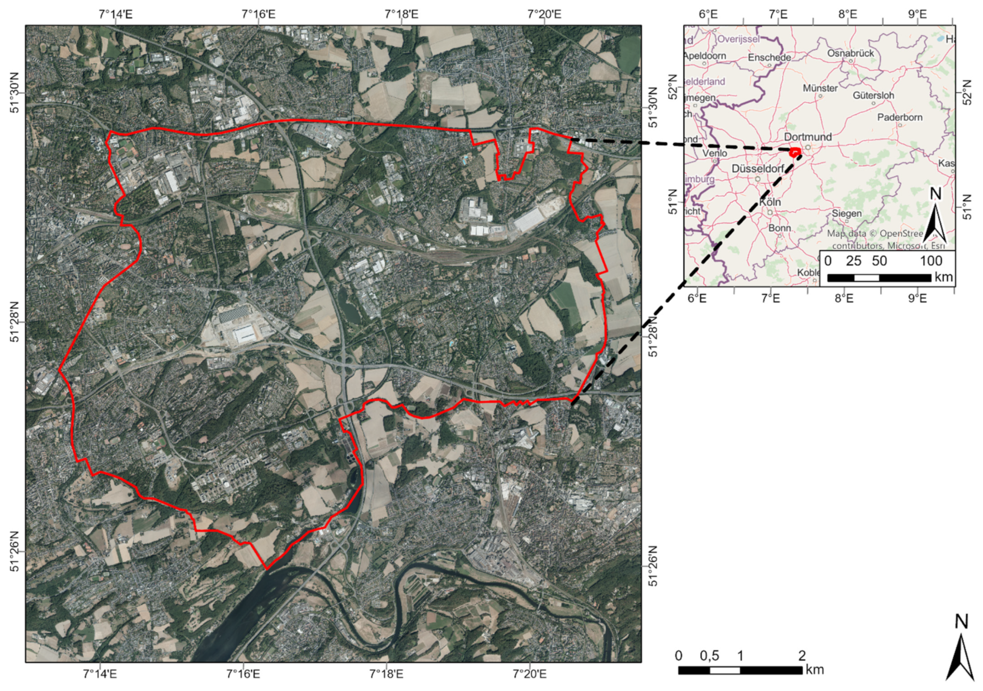
2.1. Study Area
2.2. Spatial Data

| Specifications\Data | Building Footprints (BF) | Normalized Digital Surface Model (nDSM) | Digital Orthophotos (DOP) | Global Urban Footprint (GUF) | World Settlement Footprint (WSF) |
|---|---|---|---|---|---|
| Coverage | NRW | NRW | NRW | Global (60–75° N) | Global (74° N–56° S) |
| Spatial resolution | 1:1 | 50 cm | 10 cm | 12 m (0.4″) | 10 m |
| Temporal reference | 2020 | 2018–2019 | 2018 | 2011–2012 | 2015–2019 |
| Output data | ALKIS-objects | Dense-Image-Matching based on digital aerial photos and lidar data | Orthorectified digital aerial photos | 180,000 intensity images 3m ground resolution (spotlight mode) from TerraSAR-X SAR 2018: Sentinel-1 & -2 | 217,000 Landsat-8 and 107,000 Sentinel-1 images, High Resolution Settlement Layer (HRSL) Digital Globe VHR satellite imagery and publicly released at 30 m, 2019 Sentinel-1 1,2 Mio. and Sentinel-2 1,8 Mio. |
| Position projection—Reference System EPSG | 4647 | 25,832 | 25,832 | 4326 | 4326 |
| Height projection— Reference System EPSG | / | 7837 | 7837 | / | / |
| Data format | SHP | TIF | TIF | TIF | TIF |
| Typology/Class/Attribute | Official community ID, object ID, building function, update date | Height of Objects Above surface | R, G, B, IR | Urban, open area | Urban, open area |
| Version | / | / | / | 2 | 2 |
| Geometric resolution Scale | / | ±5 dm in position and height | ±2–3 dm | / | / |
| Thematic accuracy | / | / | / | 85% | 100–75% |
| Production time | 2020 | 2018 | 2018 | 2016–2018 | 2015/2019 |
| Accessibility | Open data | Open data | Open data | Free Request for non-commercial used | Free Request for non-commercial used |
| License | Datenlizenz Deutschland–Zero–Version 2.0 | Datenlizenz Deutschland–Zero–Version 2.0 | Datenlizenz Deutschland–Zero–Version 2.0 | Research: free of charge | Research: free of charge |
| Source-Responsible organisation | GEOBASIS NRW | GEOBASIS NRW | GEOBASIS NRW | DLR | DLR |
| Reference | [53] | [54] | [49] | [61] | [57,59] |
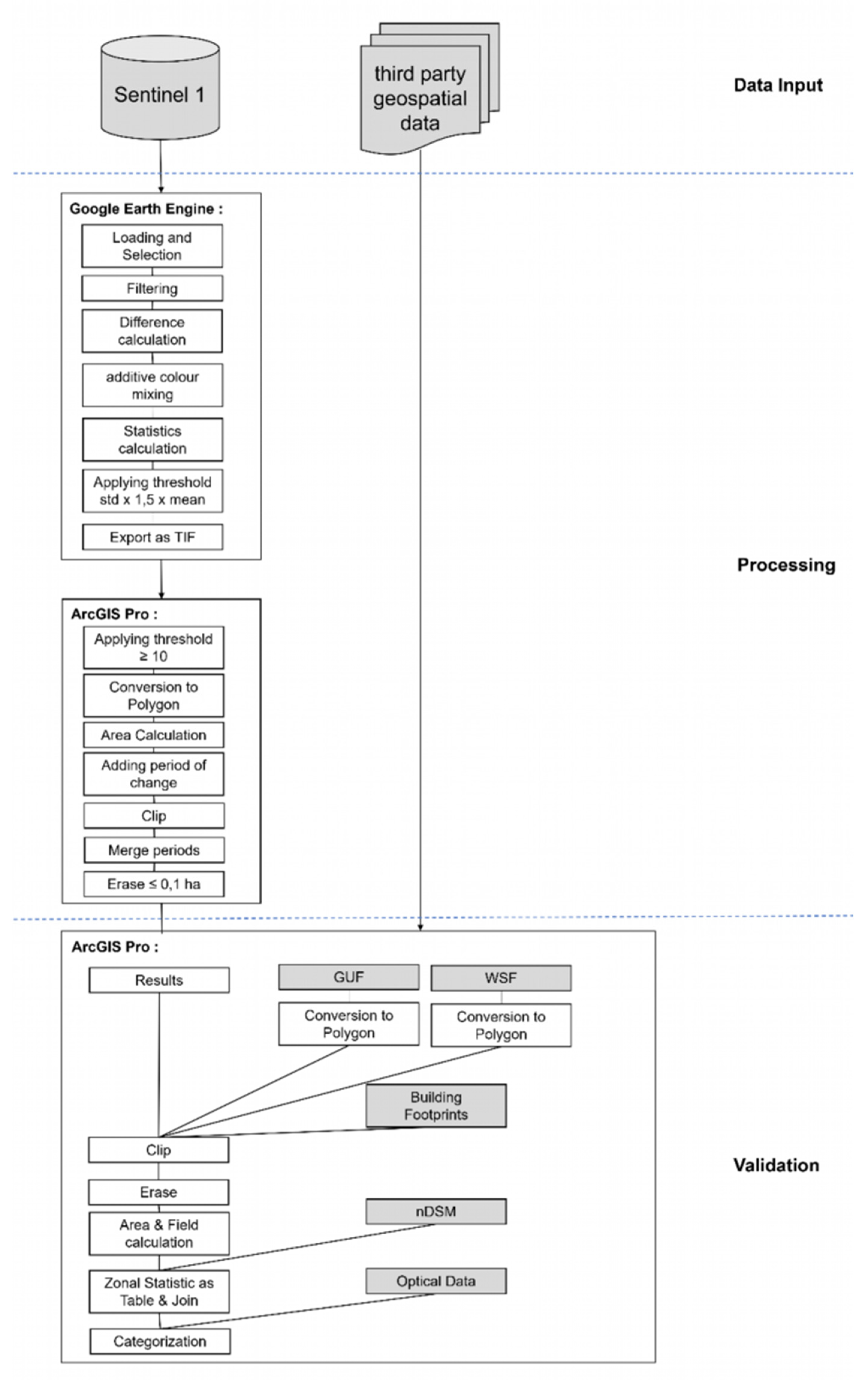
2.3. Methodology
- -
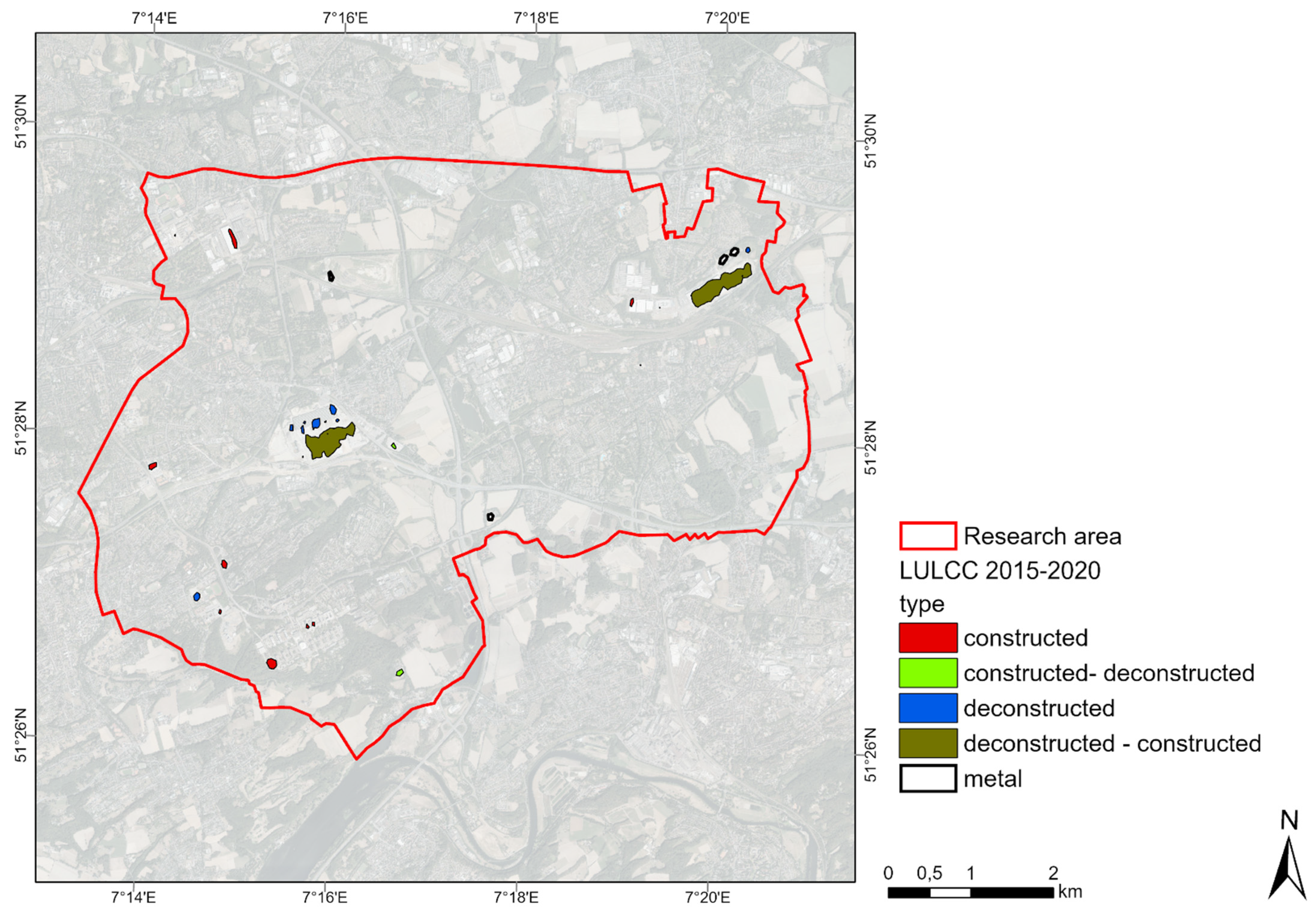
- New buildings (constructed), e.g., university buildings or dormitories;
- -
- Building demolition (deconstructed), e.g., former Opel factory buildings;
- -
- Building demolition and subsequent new construction on the same area (deconstructed–constructed), e.g., on the southern area of Opel plant I by DHL distribution centre;
- -
- SAR interaction with metallic objects on the ground surface (metal), e.g., different number and location of containers.
- -
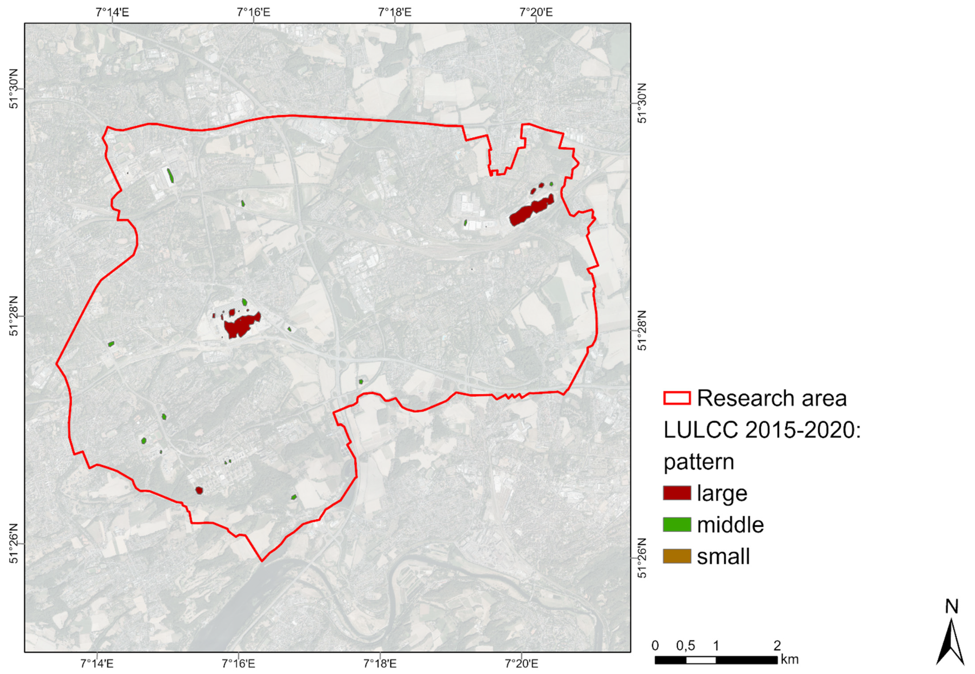
- large areas (large) (>1 ha),
- -
- medium-sized areas (middle) (0.1–1 ha),
- -
- small areas (small) (<0.1 ha).
- Compared to existing land cover change methods, the MDADT Method uses only SAR data.
- This data is analysed in a freely available cloud from Google Earth Engine, Infrastructure as a Service.
- The MDADT method is very easy to program in the cloud.
- The result is used for long term civil land cover changes of buildings, not like other methods for oil spills, flood plains and vehicles etc.
- Compared to Che & Gamba 2021 [62], the buildings are validated in the global north.
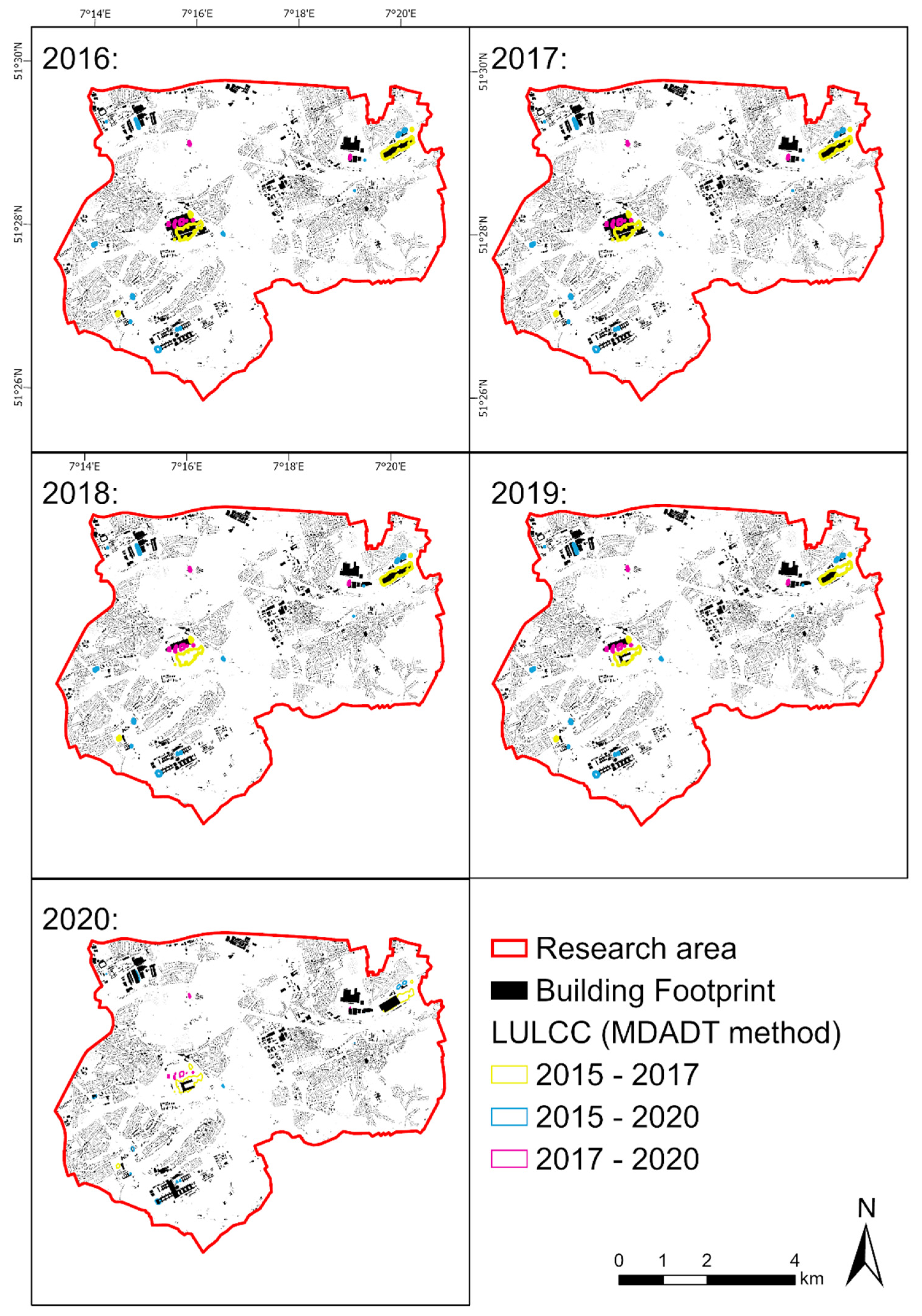
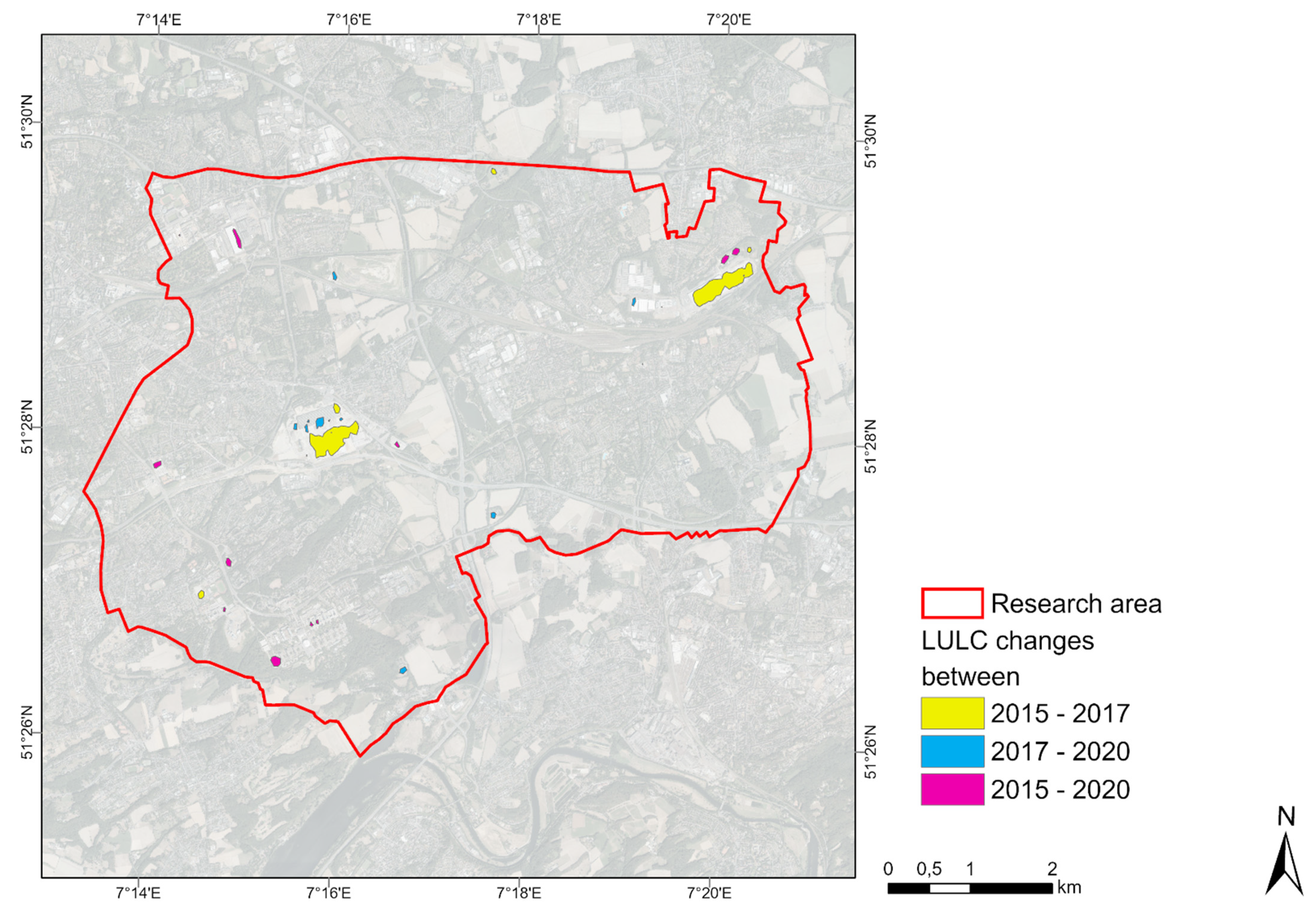
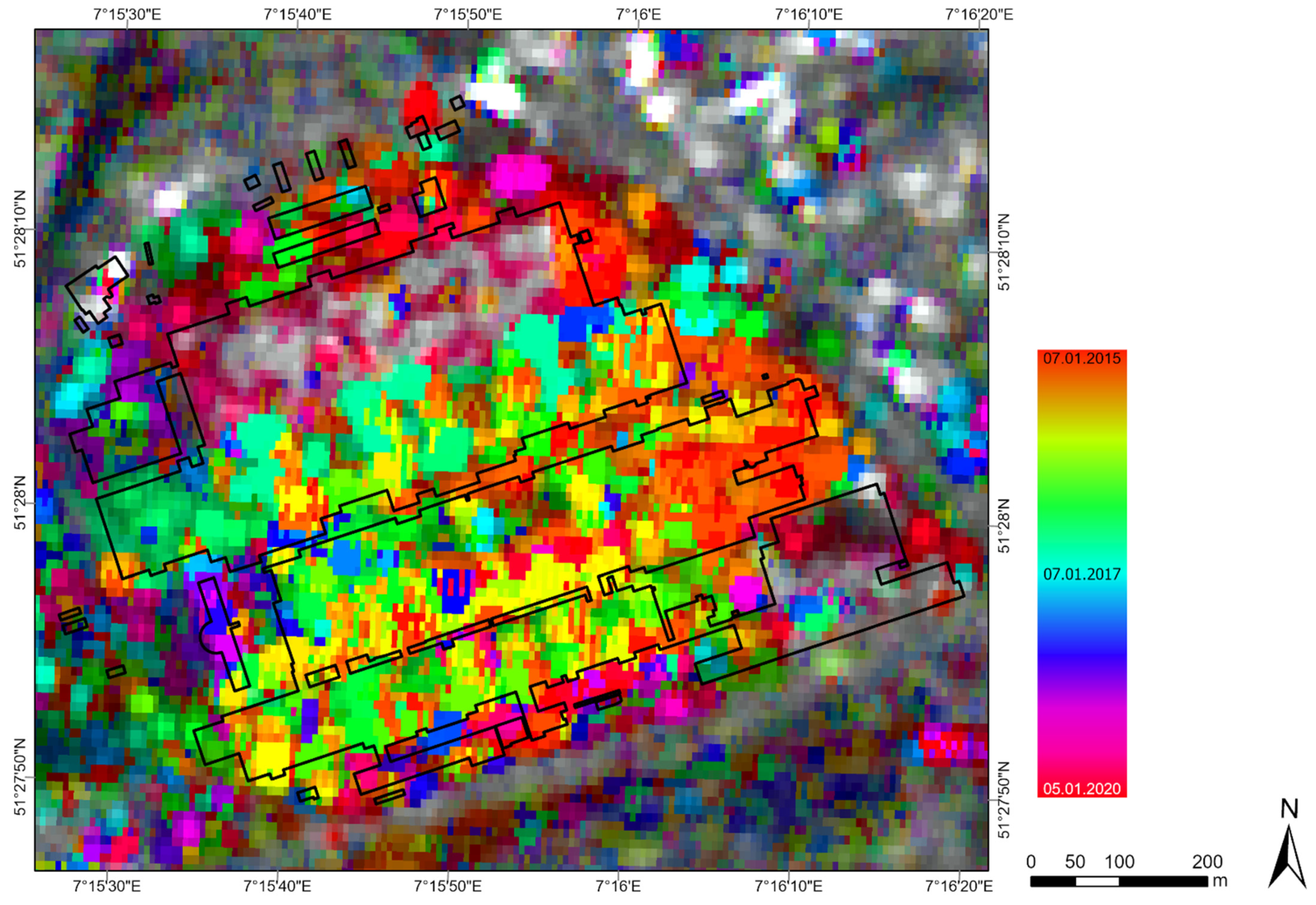
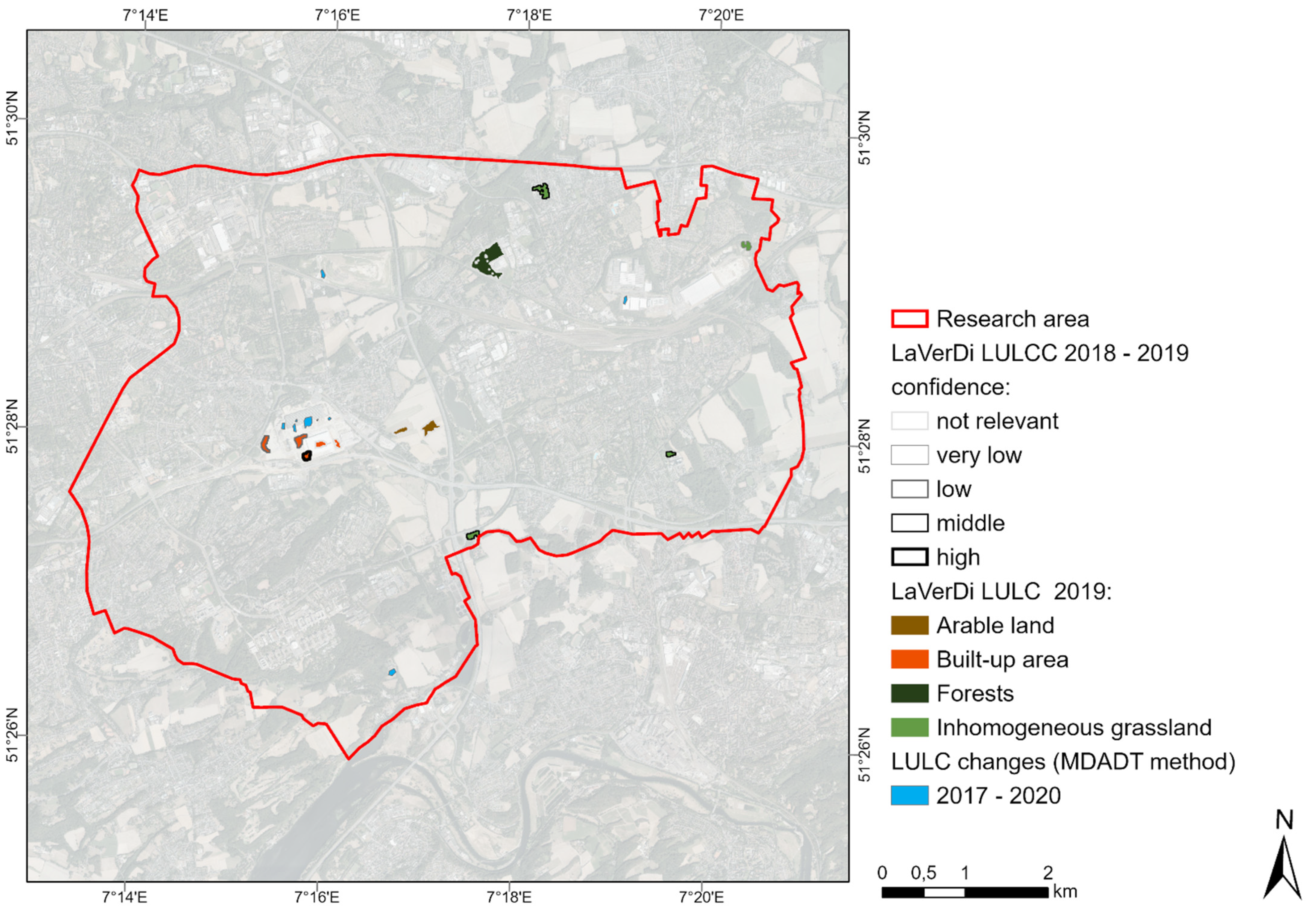
- In addition, this allows for multitemporal coverage of land cover changes over large areas and long time periods (see Figure 4). Thus, like the MDADT method, it can also be performed on an occasion-by-occasion basis.
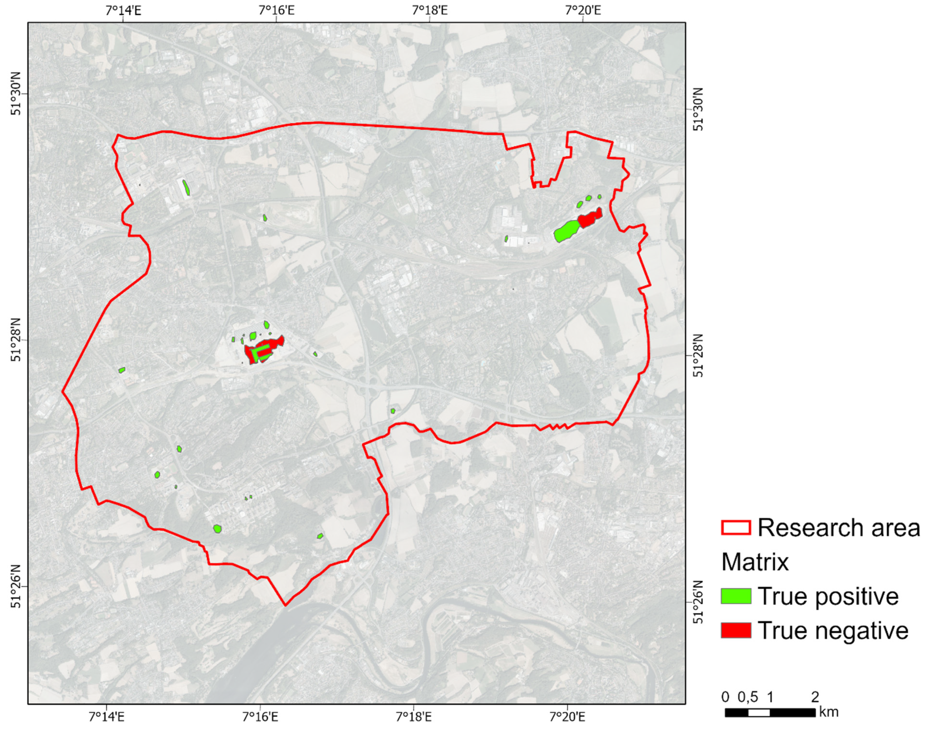
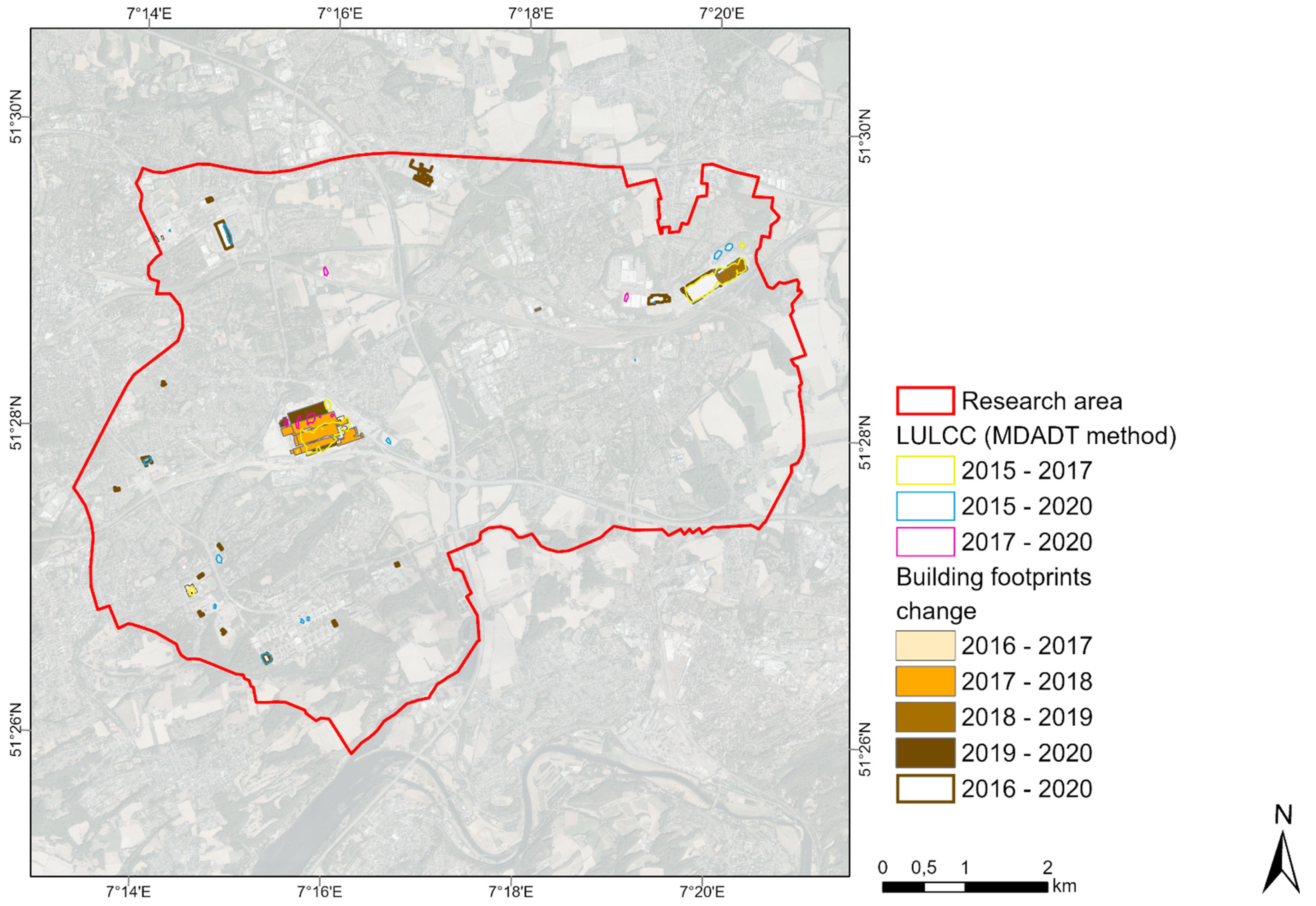
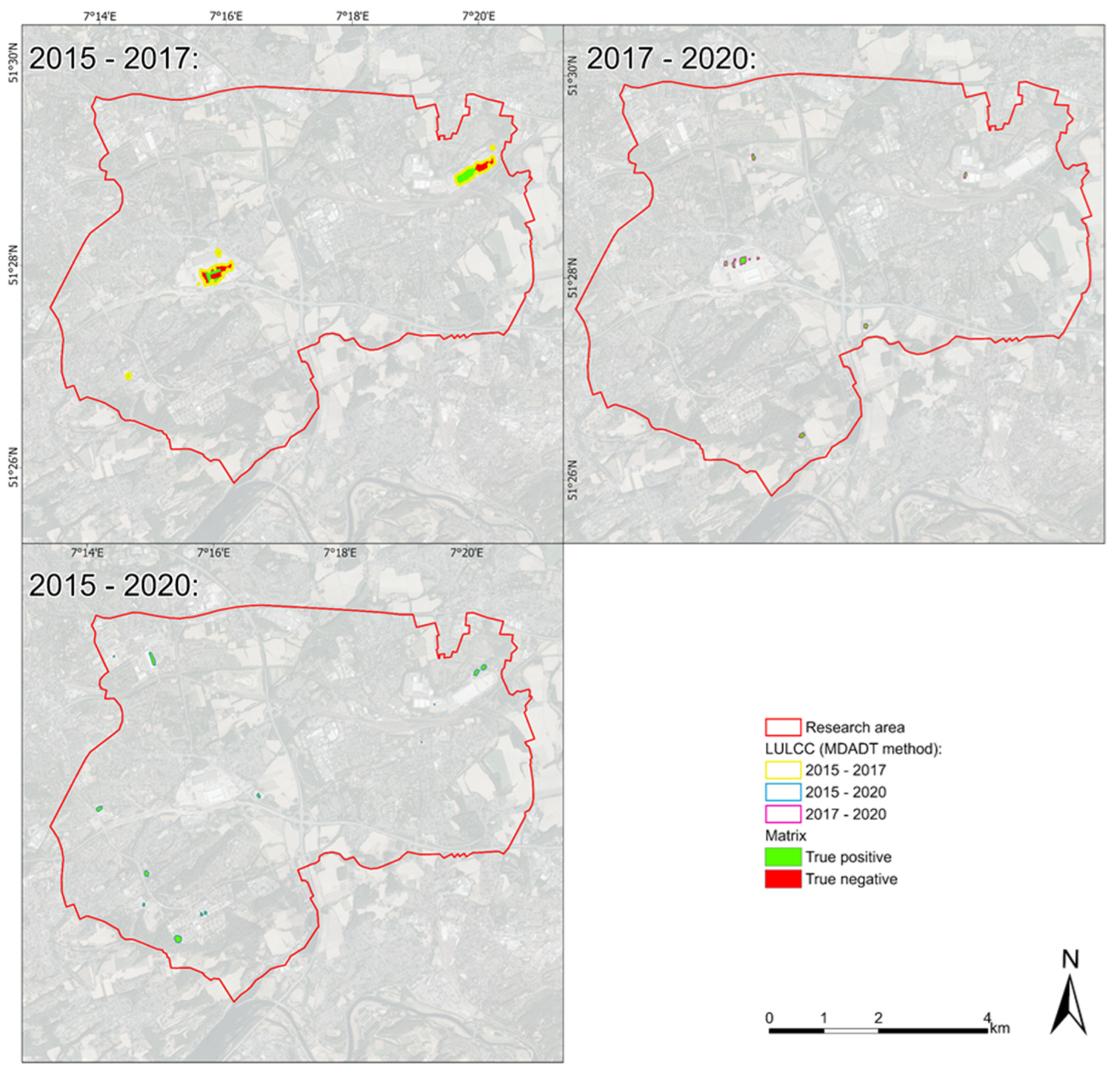
- The validation of the results takes place with the help of freely available geospatial data (Section 2.2 Spatial Data).
- The results even allow a verification of the actual validation data.
- Furthermore, the very accurate results allow to show conclusions about the urban form and the validation data (Section 3 Results).
3. Results
4. Discussion
5. Conclusions
Author Contributions
Funding
Institutional Review Board Statement
Informed Consent Statement
Conflicts of Interest
References
- Mumford, L. The Natural History of Urbanization The Emergence of the City. Man’s Role Chang. Face Earth 1956, 1, 382–398. [Google Scholar]
- Bairoch, P. Cities and Economic Development: From the Dawn of History to the Present, 2nd ed.; University of Chicago Press: Chicago, IL, USA, 1988. [Google Scholar]
- Anderson, W.P.; Kanaroglou, P.S.; Miller, E.J. Urban Form, Energy and the Environment: A Review of Issues, Evidence and Policy. Urban Stud. 1996, 33, 7–35. [Google Scholar] [CrossRef]
- Rodrigue, J.P.; Comtois, C.; Slack, B. The Geography of Transport Systems, 3rd ed.; Routledge: Oxon, UK, 2013; ISBN 9781317210108. [Google Scholar]
- Dempsey, N.; Brown, C.; Raman, S.; Porta, S.; Jenks, M.; Jones, C.; Bramley, G. Elements of Urban Form. In Dimensions of the Sustainable City; Springer: Dordrecht, The Netherlands, 2010; pp. 21–51. [Google Scholar]
- Dieleman, F.; Wegener, M. Compact City and Urban Sprawl. Built Environ. 2004, 30, 308–323. [Google Scholar] [CrossRef] [Green Version]
- Frank, L.D.; Engelke, P.O. The Built Environment and Human Activity Patterns: Exploring the Impacts of Urban Form on Public Health. J. Plan. Lit. 2001, 16, 202–218. [Google Scholar] [CrossRef]
- Dempsey, N.; Brown, C.; Bramley, G. The Key to Sustainable Urban Development in UK Cities? The Influence of Density on Social Sustainability. Prog. Plan. 2012, 77, 89–141. [Google Scholar] [CrossRef]
- Batty, M. The New Science of Cities; The MIT Press: Cambridge, UK, 2013. [Google Scholar]
- Wentz, E.A.; York, A.M.; Alberti, M.; Conrow, L.; Fischer, H.; Inostroza, L.; Jantz, C.; Pickett, S.T.A.; Seto, K.C.; Taubenböck, H. Six Fundamental Aspects for Conceptualizing Multidimensional Urban Form: A Spatial Mapping Perspective. Landsc. Urban Plan. 2018, 179, 55–62. [Google Scholar] [CrossRef]
- Rashed, T.; Jürgens, C. Remote Sensing of Urban and Suburban Areas; Springer: Dordrecht, The Netherlands, 2010. [Google Scholar]
- Netzband, M.; Jürgens, C. Urban and Suburban Areas as a Research Topic for Remote Sensing. In Remote Sensing and Digital Image Processing; Rashed, T., Jürgens, C., Eds.; Springer: Dordrecht, The Netherlands, 2010; Volume 10, pp. 1–9. [Google Scholar]
- Jürgens, C. Change Detection-Erfahrungen Bei Der Vergleichenden Multitemporalen Satellitenbildauswertung in Mitteleuropa. Photogramm. Fernerkund. Geoinf. (PFG) 2000, 1, 5–18. [Google Scholar]
- Pohl, C.; van Genderen, J.L. Review Article Multisensor Image Fusion in Remote Sensing: Concepts, Methods and Applications; Taylor & Francis: London, UK, 1998; Volume 19, ISBN 0143116982157. [Google Scholar]
- Notti, D.; Giordan, D.; Caló, F.; Pepe, A.; Zucca, F.; Galve, J.P. Potential and Limitations of Open Satellite Data for Flood Mapping. Remote Sens. 2018, 10, 1673. [Google Scholar] [CrossRef] [Green Version]
- Ferretti, A.; Prati, C.; Rocca, F. Permanent Scatterers in SAR Interferometry. IEEE Trans. Geosci. Remote Sens. 2001, 39, 8–20. [Google Scholar] [CrossRef]
- Koeniguer, E.C.; Nicolas, J.M. Change Detection Based on the Coefficient of Variation in SAR Time-Series of Urban Areas. Remote Sens. 2020, 12, 2089. [Google Scholar] [CrossRef]
- Amitrano, D.; di Martino, G.; Iodice, A.; Riccio, D.; Ruello, G. Small Reservoirs Extraction in Semiarid Regions Using Multitemporal Synthetic Aperture Radar Images. IEEE J. Sel. Top. Appl. Earth Obs. Remote Sens. 2017, 10, 3482–3492. [Google Scholar] [CrossRef]
- Brunner, D.; Lemoine, G.; Bruzzone, L. Earthquake Damage Assessment of Buildings Using VHR Optical and SAR Imagery. IEEE Trans. Geosci. Remote Sens. 2010, 48, 2403–2420. [Google Scholar] [CrossRef] [Green Version]
- Cian, F.; Marconcini, M.; Ceccato, P. Normalized Difference Flood Index for Rapid Flood Mapping: Taking Advantage of EO Big Data. Remote Sens. Environ. 2018, 209, 712–730. [Google Scholar] [CrossRef]
- Reiche, J.; Verbesselt, J.; Hoekman, D.; Herold, M. Fusing Landsat and SAR Time Series to Detect Deforestation in the Tropics. Remote Sens. 2015, 156, 276–293. [Google Scholar] [CrossRef]
- Kellndorfer, J. SAR Training Workshop for Forest Applications Part 1-Getting to Know SAR Images and Forest Signatures Software Installation and Data Sets Importing Relevant Python Packages; SERVIR Global Science Coordination Office, National Space Science and Technology Center: Huntsville, AL, USA, 2019; ISBN 1920151117.
- Inglacla, J.; Mercier, G. A New Statistical Similarity Measure for Change Detection in Multitemporal SAR Images and Its Extension to Multiscale Change Analysis. IEEE Trans. Geosci. Remote Sens. 2007, 45, 1432–1445. [Google Scholar] [CrossRef] [Green Version]
- Amitrano, D.; di Martino, G.; Guida, R.; Iervolino, P.; Iodice, A.; Papa, M.N.; Riccio, D.; Ruello, G. Earth Environmental Monitoring Using Multi-Temporal Synthetic Aperture Radar: A Critical Review of Selected Applications. Remote Sens. 2021, 13, 604. [Google Scholar] [CrossRef]
- Quin, G.; Pinel-Puyssegur, B.; Nicolas, J.M.; Loreaux, P. MIMOSA: An Automatic Change Detection Method for Sar Time Series. IEEE Trans. Geosci. Remote Sens. 2014, 52, 5349–5363. [Google Scholar] [CrossRef]
- Coombs, W.T.; Algina, J.; Oltman, D.O. Univariate and Multivariate Omnibus Hypothesis Tests Selected to Control Type I Error Rates When Population Variances Are Not Necessarily Equal. Rev. Educ. Res. 1996, 66, 137–179. [Google Scholar] [CrossRef]
- Conradsen, K.; Nielsen, A.A.; Skriver, H. Determining the Points of Change in Time Series of Polarimetric SAR Data. IEEE Trans. Geosci. Remote Sens. 2016, 54, 3007–3024. [Google Scholar] [CrossRef] [Green Version]
- Rutkowski, J.; Canty, M.J.; Nielsen, A.A. Topical Papers Site Monitoring with Sentinel-1 Dual Polarization SAR Imagery Using Google Earth Engine. J. Nucl. Mater. Manag. 2018, XLVI, 48–59. [Google Scholar]
- Muro, J.; Strauch, A.; Fitoka, E.; Tompoulidou, M.; Thonfeld, F. Mapping Wetland Dynamics with SAR-Based Change Detection in the Cloud. IEEE Geosci. Remote Sens. Lett. 2019, 16, 1536–1539. [Google Scholar] [CrossRef]
- Li, Y.; Martinis, S.; Wieland, M.; Schlaffer, S.; Natsuaki, R. Urban Flood Mapping Using SAR Intensity and Interferometric Coherence via Bayesian Network Fusion. Remote Sens. 2019, 11, 2231. [Google Scholar] [CrossRef] [Green Version]
- D’Addabbo, A.; Refice, A.; Pasquariello, G.; Lovergine, F.P.; Capolongo, D.; Manfreda, S. A Bayesian Network for Flood Detection Combining SAR Imagery and Ancillary Data. IEEE Trans. Geosci. Remote Sens. 2016, 54, 3612–3625. [Google Scholar] [CrossRef]
- D’Addabbo, A.; Refice, A.; Lovergine, F.P.; Pasquariello, G. DAFNE: A Matlab Toolbox for Bayesian Multi-Source Remote Sensing and Ancillary Data Fusion, with Application to Flood Mapping. Comput. Geosci. 2018, 112, 64–75. [Google Scholar] [CrossRef]
- Eilander, D.; Annor, F.O.; Iannini, L.; van de Giesen, N. Remotely Sensed Monitoring of Small Reservoir Dynamics: A Bayesian Approach. Remote Sens. 2014, 6, 1191–1210. [Google Scholar] [CrossRef] [Green Version]
- Amitrano, D.; Cecinati, F.; di Martino, G.; Iodice, A.; Mathieu, P.P.; Riccio, D.; Ruello, G. Feature Extraction from Multitemporal SAR Images Using Selforganizing Map Clustering and Object-Based Image Analysis. IEEE J. Sel. Top. Appl. Earth Obs. Remote Sens. 2018, 11, 1556–1570. [Google Scholar] [CrossRef]
- Lehmann, E.A.; Caccetta, P.A.; Zhou, Z.S.; McNeill, S.J.; Wu, X.; Mitchell, A.L. Joint Processing of Landsat and ALOS-PALSAR Data for Forest Mapping and Monitoring. IEEE Trans. Geosci. Remote Sens. 2012, 50, 55–67. [Google Scholar] [CrossRef]
- Errico, A.; Angelino, C.V.; Cicala, L.; Persechino, G.; Ferrara, C.; Lega, M.; Vallario, A.; Parente, C.; Masi, G.; Gaetano, R.; et al. Detection of Environmental Hazards through the Feature-Based Fusion of Optical and SAR Data: A Case Study in Southern Italy. Int. J. Remote Sens. 2015, 36, 3345–3367. [Google Scholar] [CrossRef] [Green Version]
- Dasgupta, A.; Grimaldi, S.; Ramsankaran, R.A.A.J.; Pauwels, V.R.N.; Walker, J.P. Towards Operational SAR-Based Flood Mapping Using Neuro-Fuzzy Texture-Based Approaches. Remote Sens. Environ. 2018, 215, 313–329. [Google Scholar] [CrossRef]
- Liu, Z.; Li, G.; Mercier, G.; He, Y.; Pan, Q. Change Detection in Heterogenous Remote Sensing Images via Homogeneous Pixel Transformation. IEEE Trans. Image Processing 2018, 27, 1822–1834. [Google Scholar] [CrossRef] [PubMed]
- Ganesan, P.; Rajini, V. Assessment of Satellite Image Segmentation in RGB and HSV Color Space Using Image Quality Measures. In Proceedings of the 2014 International Conference on Advances in Electrical Engineering, ICAEE 2014, Vellore, India, 9–11 January 2014; pp. 1–5. [Google Scholar] [CrossRef]
- Agapiou, A. Multi-Temporal Change Detection Analysis of Vertical Sprawl over Limassol City Centre and Amathus Archaeological Site in Cyprus during 2015–2020 Using the Sentinel-1 Sensor and the Google Earth Engine Platform. Sensors 2021, 21, 1884. [Google Scholar] [CrossRef] [PubMed]
- Olthof, I.; Fraser, R.H. Detecting Landscape Changes in High Latitude Environments Using Landsat Trend Analysis: 2. Classification. Remote Sens. 2014, 6, 11558–11578. [Google Scholar] [CrossRef] [Green Version]
- Small, C.; Sousa, D. Humans on Earth: Global Extents of Anthropogenic Land Cover from Remote Sensing. Anthropocene 2016, 14, 1–33. [Google Scholar] [CrossRef] [Green Version]
- Charrier, L.; Godet, P.; Rambour, C.; Weissgerber, F.; Erdmann, S.; Koeniguer, E.C. Analysis of Dense Coregistration Methods Applied to Optical and SAR Time-Series for Ice Flow Estimations. In Proceedings of the 2020 IEEE Radar Conference (RadarConf20), Florence, Italy, 21–25 September 2020; pp. 6–11. [Google Scholar] [CrossRef]
- Gorelick, N.; Hancher, M.; Dixon, M.; Ilyushchenko, S.; Thau, D.; Moore, R. Google Earth Engine: Planetary-Scale Geospatial Analysis for Everyone. Remote Sens. Environ. 2017, 202, 18–27. [Google Scholar] [CrossRef]
- Mutanga, O.; Kumar, L. Google Earth Engine Applications. Remote Sens. 2019, 11, 591. [Google Scholar] [CrossRef] [Green Version]
- Henits, L.; Jürgens, C.; Mucsi, L. Seasonal Multitemporal Land-Cover Classification and Change Detection Analysis of Bochum, Germany, Using Multitemporal Landsat TM Data. Int. J. Remote Sens. 2016, 37, 3439–3454. [Google Scholar] [CrossRef]
- Zepp, H.; Inostroza, L. Who Pays the Bill? Assessing Ecosystem Services Losses in an Urban Planning Context. Land 2021, 10, 369. [Google Scholar] [CrossRef]
- ESRI OpenStreetMap Contributors v2 (c), Microsoft, Contributors, Esri Community Maps. Available online: https://cdn.arcgis.com/sharing/rest/content/items/3e1a00aeae81496587988075fe529f71/resources/styles/root.json (accessed on 1 February 2022).
- Land NRW-Digitale Orthophotos-Dl-de/Zero-2-0. Available online: https://www.bezreg-koeln.nrw.de/brk_internet/geobasis/luftbildinformationen/aktuell/digitale_orthophotos/index.html (accessed on 1 February 2022).
- Google Developers Sentinel-1 SAR GRD: C-Band Synthetic Aperture Radar Ground Range Detected, Log Scaling. Available online: https://developers.google.com/earth-engine/datasets/catalog/COPERNICUS_S1_GRD (accessed on 1 February 2022).
- ESA. ESA’s Radar Observatory Mission for GMES Operational Services; ESA Communications: Leiden, The Netherlands, 2012; Volume 1, ISBN 9789292214180. [Google Scholar]
- ESA Copernicus Open Access Hub. Available online: https://scihub.copernicus.eu/dhus/#/home (accessed on 1 February 2022).
- Land NRW-Hausumringe HU NW-Dl-de/Zero-2-0. Available online: https://www.opengeodata.nrw.de/produkte/geobasis/lk/hu_shp/ (accessed on 1 February 2022).
- Land NRW-Normalisiertes Digitales Oberflächenmodell-Dl-de/Zero-2-0. Available online: https://www.bezreg-koeln.nrw.de/brk_internet/geobasis/hoehenmodelle/digitale_oberflaechenmodelle/normalisiertes_digitales_oberflaechenmodell/index.html (accessed on 1 February 2022).
- Esch, T.; Schenk, A.; Ullmann, T.; Thiel, M.; Roth, A.; Dech, S. Characterization of Land Cover Types in TerraSAR-X Images by Combined Analysis of Speckle Statistics and Intensity Information. IEEE Trans. Geosci. Remote Sens. 2011, 49, 1911–1925. [Google Scholar] [CrossRef]
- Esch, T.; Bachofer, F.; Heldens, W.; Hirner, A.; Marconcini, M.; Palacios-Lopez, D.; Roth, A.; Üreyen, S.; Zeidler, J.; Dech, S.; et al. Where We Live-A Summary of the Achievements and Planned Evolution of the Global Urban Footprint. Remote Sens. 2018, 10, 895. [Google Scholar] [CrossRef] [Green Version]
- Marconcini, M.; Metz-Marconcini, A.; Üreyen, S.; Palacios-Lopez, D.; Hanke, W.; Bachofer, F.; Zeidler, J.; Esch, T.; Gorelick, N.; Kakarla, A.; et al. Outlining Where Humans Live, the World Settlement Footprint 2015. Sci. Data 2020, 7, 242. [Google Scholar] [CrossRef] [PubMed]
- Strano, E.; Simini, F.; de Nadai, M.; Esch, T.; Marconcini, M. The Agglomeration and Dispersion Dichotomy of Human Settlements on Earth. Sci. Rep. 2020, 11, 23289. [Google Scholar] [CrossRef] [PubMed]
- Palacios-Lopez, D.; Bachofer, F.; Esch, T.; Heldens, W.; Hirner, A.; Marconcini, M.; Sorichetta, A.; Zeidler, J.; Kuenzer, C.; Dech, S.; et al. New Perspectives for Mapping Global Population Distribution Using World Settlement Footprint Products. Sustainability 2019, 11, 56. [Google Scholar] [CrossRef] [Green Version]
- Land NRW-1937–2016: Deutsche Grundkarte 1:5000-Dl-de/Zero-2-0. Available online: https://www.bezreg-koeln.nrw.de/brk_internet/geobasis/topographische_karten/historisch/1937/index.html (accessed on 1 February 2022).
- DLR GUF Data and Access. Available online: https://www.dlr.de/eoc/en/desktopdefault.aspx/tabid-11725/20508_read-47944/ (accessed on 1 February 2022).
- Che, M.; Gamba, P. Bi- and three-dimensional urban change detection using sentinel-1 SAR temporal series. GeoInformatica 2021, 25, 759–773. [Google Scholar] [CrossRef]
- Juergens, C.; Meyer-Heß, M.F. Identification of Construction Areas from VHR-Satellite Images for Macroeconomic Forecasts. Remote Sens. 2021, 13, 2618. [Google Scholar] [CrossRef]
- Di Martino, T.; Colin-Koeniguer, E.; Guinvarch, R.; Thirion-Lefevre, L. REACTIV Algorithm. arXiv 2020, arXiv:1904.11335v2. [Google Scholar]
- Koeniguer, E.C. REACTIV Code. Available online: https://code.earthengine.google.com/29923deb406fd4803a9b8963cdb50a12 (accessed on 1 February 2022).
- Geobasis NRW Informationen Zur Bearbeitung von Gemeldeten Kartenfehlern. 2020, pp. 1–4. Available online: https://www.bezreg-koeln.nrw.de/brk_internet/tim-online/timonline_information_tim_bearbeitung_kartenfehler.pdf (accessed on 1 February 2022).
- Knöfel, P.; BKG; Herrmann, D. GAF Projekt Landschafts Ver Änderungs Dienst. 2020. Available online: https://subs.emis.de/LNI/Proceedings/Proceedings238/P-238.pdf (accessed on 1 February 2022).
- BKG; Geodäsie, B. Für K. und Landschaftsveränderungsdienst (LaVerDi). Available online: https://gdz.bkg.bund.de/index.php/default/landschaftsveraenderungsdienst.html (accessed on 1 February 2022).
- Knöfel, P.; BKG. Vorstellung Des LandschaftsVeränderungsDienstes Des BKG-LaVerDi LaVerDi–Landschaftsveränderungsdienst Hauptziel: Kontinuierliche und Automatisierte Analyse von Landschaftsveränderungen Mit. 2020. Available online: https://www.d-geo.de/arbeitstreffen/47/P15_Kn%C3%B6fel_LaVerDi.pdf (accessed on 1 February 2022).
- Chini, M.; Pelich, R.; Hostache, R.; Matgen, P.; Lopez-Martinez, C. Towards a 20 m Global Building Map from Sentinel-1 SAR Data. Remote Sens. 2018, 10, 1833. [Google Scholar] [CrossRef] [Green Version]


| Specifications | Sentinel-1 |
|---|---|
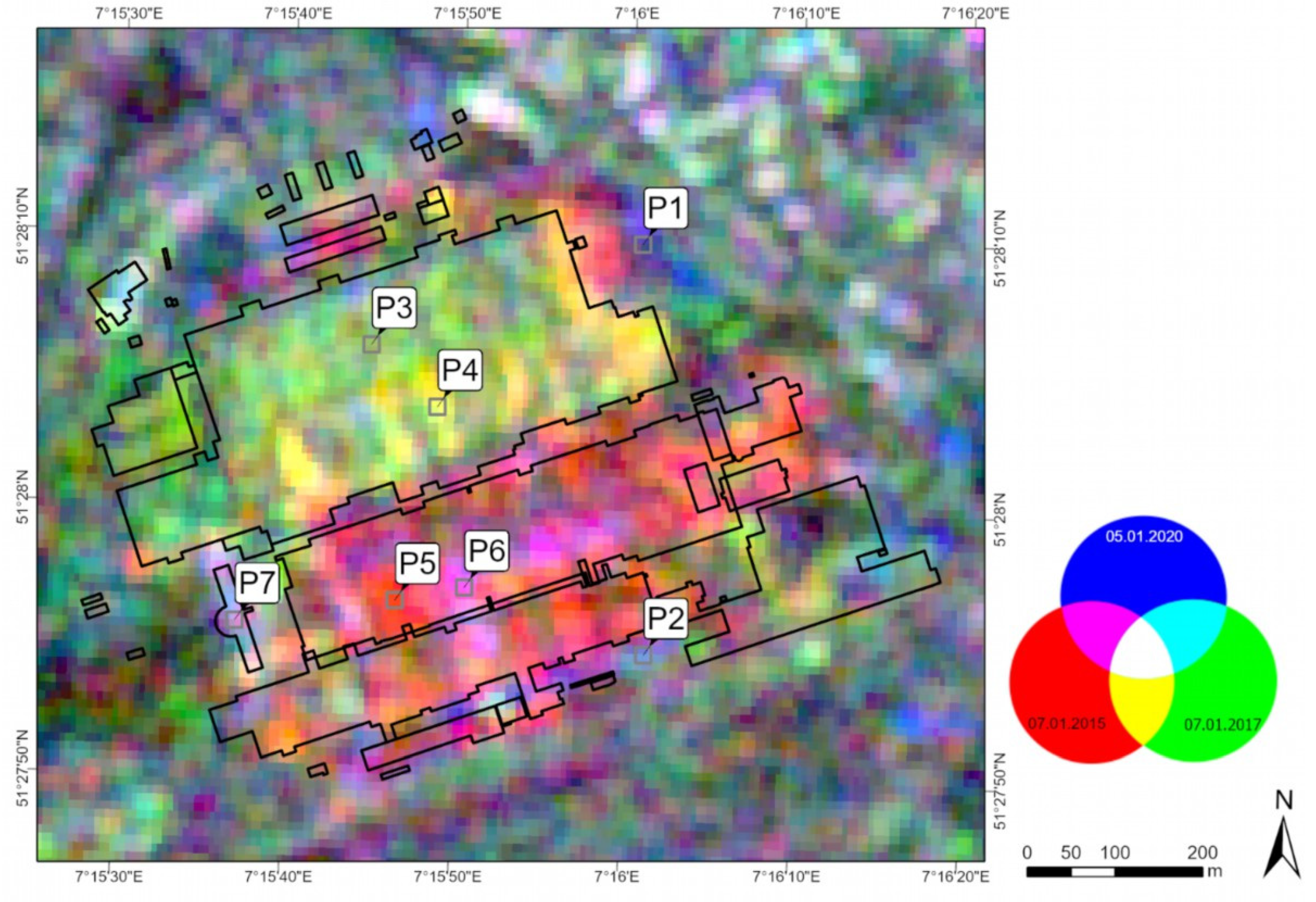
| Dates and time (YYYY-MM-DD) | A 7 January 2015, 4:41:45 a.m. B 7 January 2017, 4:49:26 a.m. A 5 January 2020, 4:42:06 a.m. |
| Ground Resolution in m | 10 |
| Azimuth Resolution in m | 20 |
| moderate geometric resolution | 5 m by 20 m |
| Polarization | Dual (VV–VH) |
| Frequency | C-Band |
| Sensor mode | IW |
| Mode | Interferometric wide (SLC) |
| Incidence Angle | 18.3°–46.8° |
| Coverage in km | >250 km × 100 km |
| Processing level: | thermal noise corrected, Radiometric calibration, Terrain correction (SRTM) and converted to decibels via log scaling (10 ∗ log10(x)). |
| Orbit direction | descending |
| Constructed | Constructed—Deconstructed | Deconstructed | Deconstructed—Constructed | Metal | Sum | ||||||
|---|---|---|---|---|---|---|---|---|---|---|---|
| True Positive | True Negative | True Positive | True Negative | True Positive | True Negative | True Positive | True Negative | True Positive | True Negative | ||
| 2015–2017 | 3 | 1 | 1 | 5 | |||||||
| 2015–2020 | 9 | 1 | 1 | 11 | |||||||
| 2017–2020 | 1 | 1 | 1 | 2 | 5 | ||||||
| sum | 10 | 0 | 2 | 0 | 4 | 0 | 1 | 1 | 3 | 0 | 21 |
| Constructed | Constructed—Deconstructed | Deconstructed | Deconstructed—Constructed | Metal | Sum | |
|---|---|---|---|---|---|---|
| 2015–2017 | 3 | 2 | 5 | |||
| 2015–2020 | 9 | 1 | 1 | 11 | ||
| 2017–2020 | 1 | 1 | 1 | 2 | 5 | |
| sum | 10 | 2 | 4 | 2 | 3 | 21 |
| Large | Middle | Small | Sum | |
|---|---|---|---|---|
| 2015–2017 | 2 | 3 | 5 | |
| 2015–2020 | 2 | 6 | 3 | 11 |
| 2017–2020 | 1 | 4 | 5 | |
| sum | 5 | 13 | 3 | 21 |
| Pattern (Area)\Type | Constructed | Deconstructed | Deconstructed—Constructed | Metal | Sum |
|---|---|---|---|---|---|
| large | 1 | 1 | 2 | 1 | 5 |
| middle | 8 | 3 | 0 | 2 | 13 |
| small | 3 | 0 | 0 | 0 | 3 |
| sum | 12 | 4 | 2 | 3 | 21 |
| Specifications\Data | LaVerDi |
|---|---|
| Coverage | Germany |
| Spatial resolution | >0.5 ha |
| Temporal reference | 2020 |
| Output data | LULCC digital Land Cover Model Germany (LBM-DE) and sentinel-2 |
| Position projection—Reference System EPSG | 4258 |
| Height projection– Reference System EPSG | / |
| Data format | SHP |
| Typology/Class/Attribute | Confidence, Land use land cover; probability of change, method, Area |
| Version | / |
| Geometric resolution Scale | / |
| Thematic accuracy | >80 |
| Production time | 2020 |
| Accessibility | Open data |
| License | not required |
| Source-Responsible organisation | BKG |
| Reference | [67,68,69] |
Publisher’s Note: MDPI stays neutral with regard to jurisdictional claims in published maps and institutional affiliations. |
© 2022 by the authors. Licensee MDPI, Basel, Switzerland. This article is an open access article distributed under the terms and conditions of the Creative Commons Attribution (CC BY) license (https://creativecommons.org/licenses/by/4.0/).
Share and Cite
Gruenhagen, L.; Juergens, C. Multitemporal Change Detection Analysis in an Urbanized Environment Based upon Sentinel-1 Data. Remote Sens. 2022, 14, 1043. https://doi.org/10.3390/rs14041043
Gruenhagen L, Juergens C. Multitemporal Change Detection Analysis in an Urbanized Environment Based upon Sentinel-1 Data. Remote Sensing. 2022; 14(4):1043. https://doi.org/10.3390/rs14041043
Chicago/Turabian StyleGruenhagen, Lars, and Carsten Juergens. 2022. "Multitemporal Change Detection Analysis in an Urbanized Environment Based upon Sentinel-1 Data" Remote Sensing 14, no. 4: 1043. https://doi.org/10.3390/rs14041043
APA StyleGruenhagen, L., & Juergens, C. (2022). Multitemporal Change Detection Analysis in an Urbanized Environment Based upon Sentinel-1 Data. Remote Sensing, 14(4), 1043. https://doi.org/10.3390/rs14041043