Rapid Vehicle Detection in Aerial Images under the Complex Background of Dense Urban Areas

Abstract

Vehicle detection on aerial remote sensing images under the complex background of urban areas has always received great attention in the field of remote sensing; however, the view of remote sensing images usually covers a large area, and the size of the vehicle is small and the background is complex. Therefore, compared with object detection in the ground view images, vehicle detection in aerial images remains a challenging problem. In this paper, we propose a single-scale rapid convolutional neural network (SSRD-Net). In the proposed framework, we design a global relational (GR) block to enhance the fusion of local and global features; moreover, we adjust the image segmentation method to unify the vehicle size in the input image, thus simplifying the model structure and improving the detection speed. We further introduce an aerial remote sensing image dataset with rotating bounding boxes (RO-ARS), which has complex backgrounds such as snow, clouds, and fog scenes. We also design a data augmentation method to get more images with clouds and fog. Finally, we evaluate the performance of the proposed model on several datasets, and the experimental results show that the recall and precision are improved compared with existing methods.

1. Introduction

With the development of remote sensing technology, the quantity of remote sensing images has also been greatly increased. Compared with aerospace remote sensing image, aerial remote sensing image has the advantages of large imaging scale, high resolution, and accurate geometric correction [1,2,3]. Therefore, aerial remote sensing is still an important remote sensing way; it usually uses airplanes or balloons as working platforms, and the flying altitude is between hundreds of meters and tens of kilometers. In aerial remote sensing images, vehicle detection is an indispensable technology in civil and military surveillance, such as traffic management and urban planning [4,5,6,7]; however, the method of manual interpretation for vehicle identification has low data utilization and poor information timeliness, which is easily affected by physical conditions, mentality, and subjective consciousness. Therefore, it is particularly necessary to perform automatic vehicle detection on remote sensing images efficiently and accurately.

Compared with general images, aerial remote sensing images have a unique perspective; this task becomes challenging due to the following reasons:

Large field of view (FOV): Aerial remote sensing images are taken by high-resolution imaging sensors, and the obtained images generally have the characteristics of a large field of view (few target pixels) and high resolution. Therefore, simply down-sampling to the input size required by most algorithms is not suitable.

Larger scale range: Since the collection height of remote sensing images and sensor parameters are different, the scales of the similar targets are also inconsistent. Generally, objects of interest in aerial images are often very small and densely clustered.

Special perspective: Aerial imagery is a top view, which makes the ground target have complete rotation invariance, and the direction angle is arbitrary. Therefore, there is no overlap of goals.

Complex background: In the urban remote sensing image, there are a large number of objects with similar characteristics as the vehicle target; moreover, the aerial images are susceptible to weather such as clouds and fog, it is necessary to consider the impact of complex weather conditions on the aerial images.

Traditional target detection algorithms [8], such as Viola Jones detectors [9,10], HOG detector [11], and deformable part model (DPM) [12,13,14,15], are usually designed for the geometric features, spatial relationships, target contours, and other features [16]. These algorithms can only achieve low accuracy, while the methods with higher accuracy, such as frame difference, can only detect vehicles in motion. Such strategy information is not very robust to the diversity of the environment, and it is difficult to well adapt to the needs of the actual scenes. Since the introduction of convolutional neural networks in the ImageNet large-scale visual recognition challenge (ILSVRC) [17,18], the network model based on deep learning has achieved remarkable results in the field of target detection. Meanwhile, the design of large, high-quality general-purpose labeled datasets, such as Pascal VOC [19,20], LVIS [21], and MS COCO [22], have also promoted the progress of target detection technology.

Within the last decades, deep learning methods have been widely used in various research fields [23,24,25,26], and the emerging development of convolutional neural networks (CNNs) brought some significant improvements. The CNN-based “two-stage” methods, such as R-FCN [27] and Faster RCNN [28], achieve state-of-the-art (SOTA) performance in terms of accuracy. In contrast, the end-to-end model, which does not require region proposals [29] has higher detection speed, such as YOLO [30,31,32,33] and SSD [34]. In addition, transformer-based detection models [35,36,37], such as DETR [38], usually have excellent global perception capabilities.

Many recent works have exploited SOTA detectors to detect, such as Faster R-CNN [27], deformable R-CNN [39], YOLOv4 [33], etc. Observing the input size of the model, the Faster RCNN model will resize the short side of the input image to 600 pixels and YOLO runs on either 608 × 608-pixel inputs. None of these models can directly receive the typical size of aerial remote sensing images (ITCVD [40]: ~5616 × 3744 pixels, DOTA [41]: ~4000 × 4000 pixels).

In order to meet the requirements of the standard architecture, it is not feasible to resize the image, because this way will lead to the loss of small pixel targets directly (MS COCO dataset definition [22]: <32 × 32 pixels). To solve the above-mentioned problems, existing algorithms usually segment the original image first. The YOLT [42] model adopts a “sliding window” method for cropping and designed a 15% overlap to ensure all regions will be analyzed; however, the size of the target object depends on the shooting height and camera parameters. Using a fixed size to crop the original image, the target pixel still has a large dynamic range, which affects the target detection ability.

There are many down-sampling layers inside the existing detection models, which will expand the receptive field. Vehicle targets in aerial remote sensing images are relatively small in size (ITCVD [40]: ~30 × 15 pixels) and have fewer features. They are submerged by background features easily, and it is difficult to extract effective feature information. Existing algorithms usually use feature fusion to improve the ability to detect small targets. Specifically, the SSD model [34] uses a pyramidal feature hierarchy and the Mask R-CNN [43] model uses Feature Pyramid Network [44] (FPN) structure. The ablation experiment shows that the model is beneficial to improve the ability to detect small targets; however, current techniques are still suboptimal in the applications of aerial images. There is a large amount of redundant information for aerial remote sensing images, which affects the detection efficiency.

In addition, several studies indicate that it is crucial for small targets detection by enhancing the fusion of contextual information. Some studies have adopted long- and short-term memory networks (LSTM) [45] and spatial memory networks (SMN) [46] to enhance target features. For instance, AC-FCN [47] pointed out that the information between targets can help improve detection capabilities, whereas, the structure of this type of method is usually complex and these methods are still simple feed-forward networks, which are easy to cause the loss of feature information; moreover, FA-SSD [48] improves the ability to extract context information from small targets by using more high-level abstract features. These methods achieve good results; however, they are not suitable for aerial images because they do not have real-time capabilities.

We also notice that the lack of data sets is another important reason why aerial images are difficult to process. The labeled boxes of some datasets do not provide directions so that there is a large amount of overlap in the labeled boxes of the dense target area; it will have a great impact on the target detection in dense areas. Research on the target detection algorithms based on deep learning is inseparable from the support of data. Many scholars have also established target detection datasets for remote sensing images, such as DOTA [41], VEDAI [49], DLR 3K [50], and so on; in fact, most of the images in the DOTA data set come from Google Earth, taken by aerospace remote sensing satellites, and such images cannot truly reflect the perspective of aerial remote sensing images. The VEDAI dataset has a small number of vehicles, sparse distribution, and simple background, all of which make vehicle targets relatively easy to detect. Although the DLR 3K dataset is more challenging and authentic, it only contains 20 aerial images. The number of images in the dataset is too few for training a convolutional neural network model.

Furthermore, for the cloud and fog phenomenon in aerial remote sensing images, there are usually two solutions: one of them is to improve the image quality through the haze removal algorithm, such as DCP (Dark Channel Prior) [51,52], MC (Maximum Contrast) [53], CAP (Color Attenuation Prior) [54], and so on. Another solution is to train pictures containing haze and constrain the features through the objective function. Nevertheless, existing haze removal algorithms usually produce a halo effect or color distortion phenomenon [55]. The existing datasets also do not include the haze phenomenon.

As described, although the performance of the above models is impressive, none of the existing frameworks can handle aerial remote sensing images well. To address these problems, we propose several prioritization schemes. The main contributions of this paper are presented as follows:

(1)

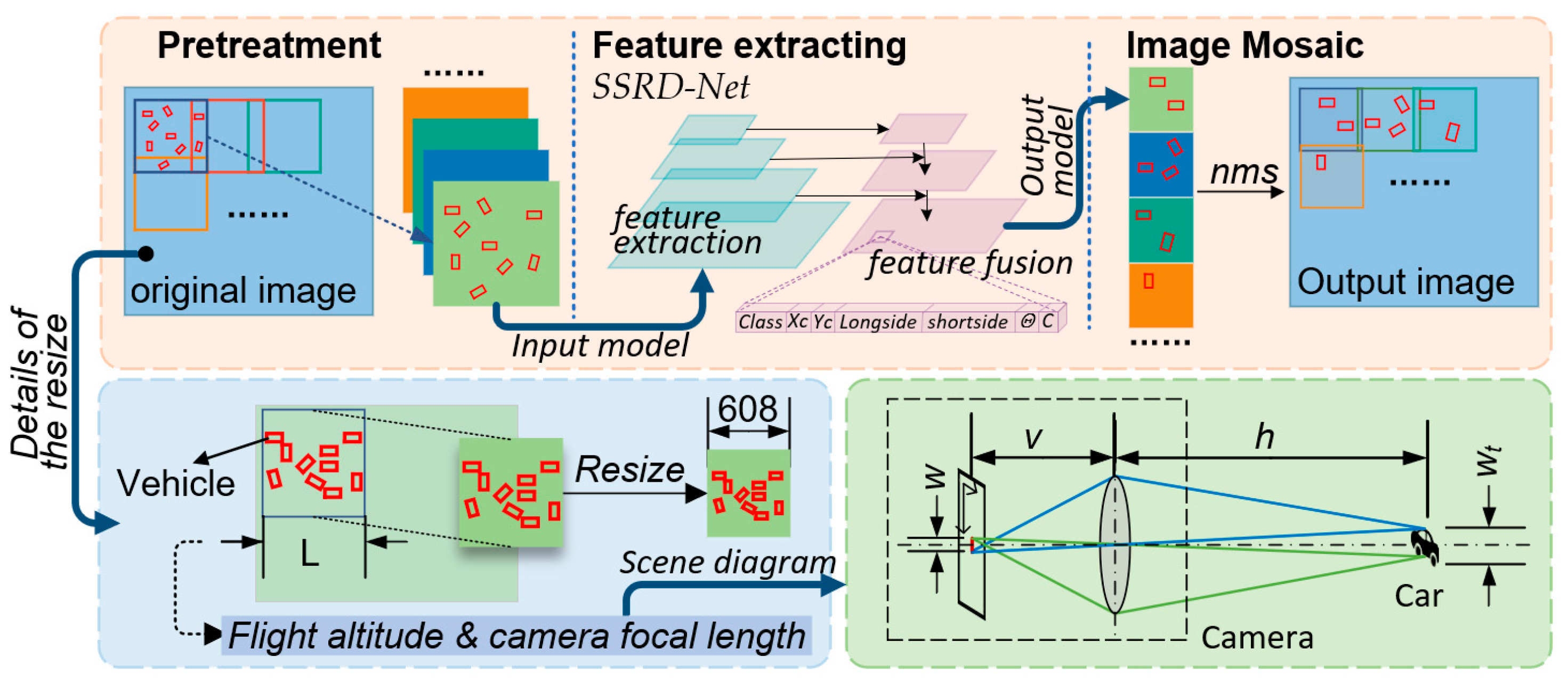
An adaptive image segmentation method based on the parameters of aerospace vehicles and cameras is proposed; this method limits the size of the target to a small range by dynamically adjusting the crop size. It plays a major role in improving the speed and accuracy of model detection.

(2)

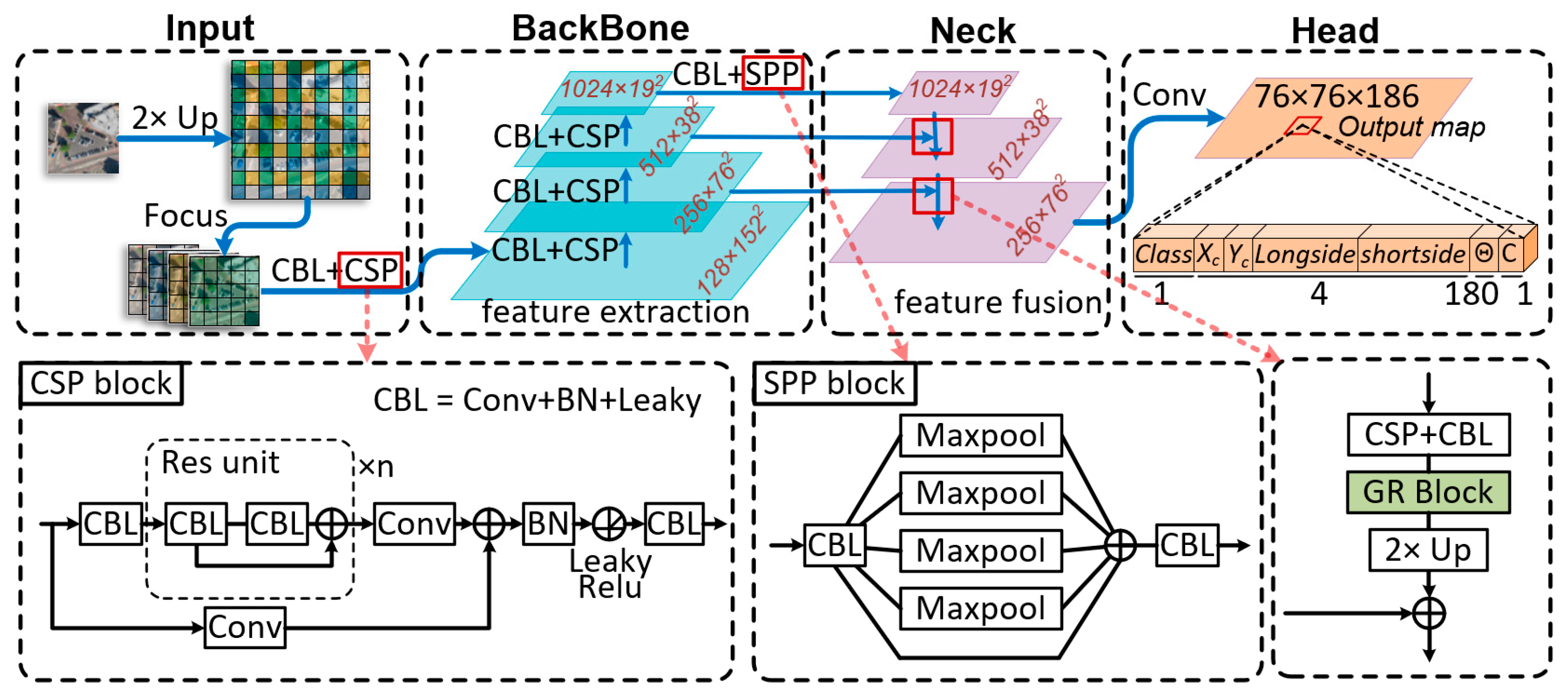
In view of the high speed and accuracy of YOLOv4 [33], this paper uses YOLOv4 as the main frame of vehicle detection. We present the single-scale rapid convolutional neural network (SSRD-Net). A structure with denser prediction anchor frames is proposed, optimizing the feature fusion structure to improve the ability to detect small targets.

(3)

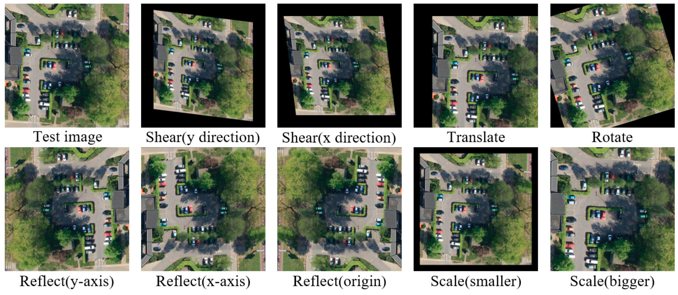
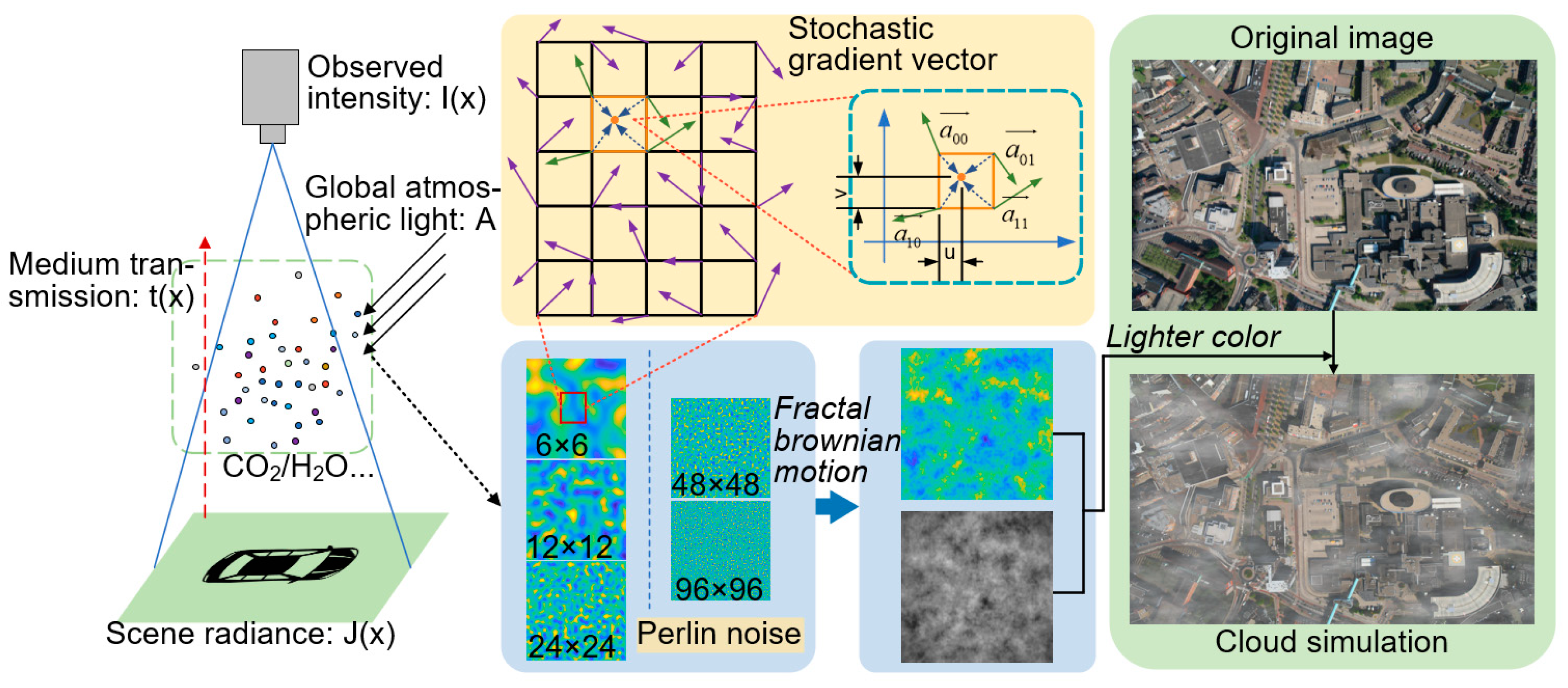
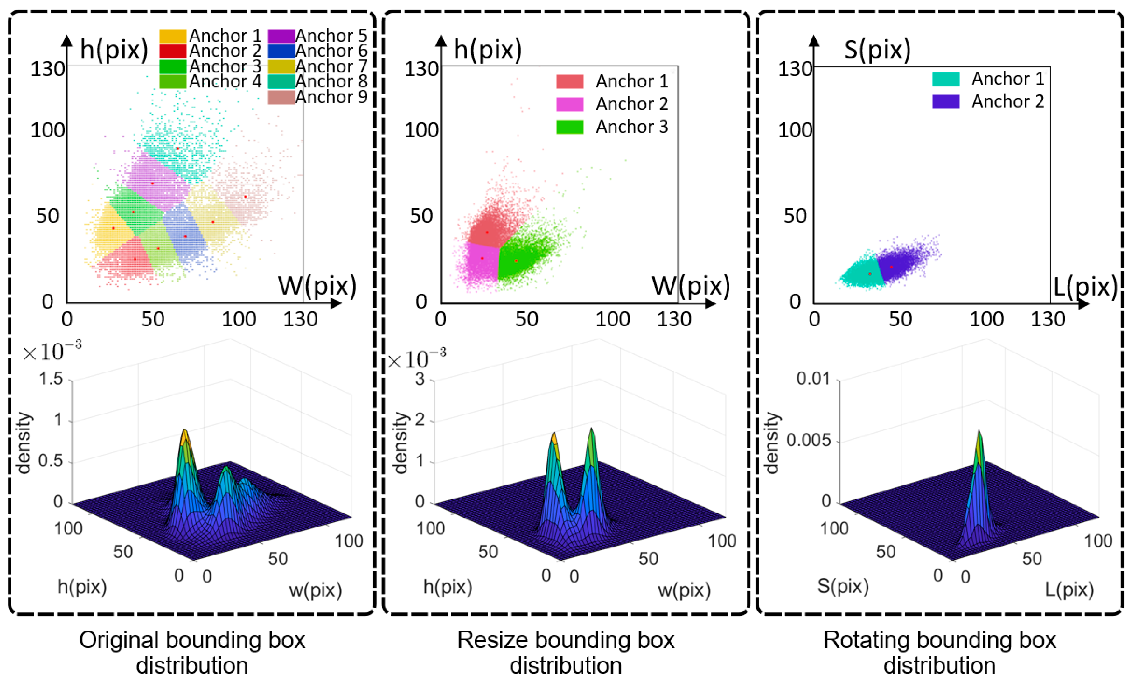
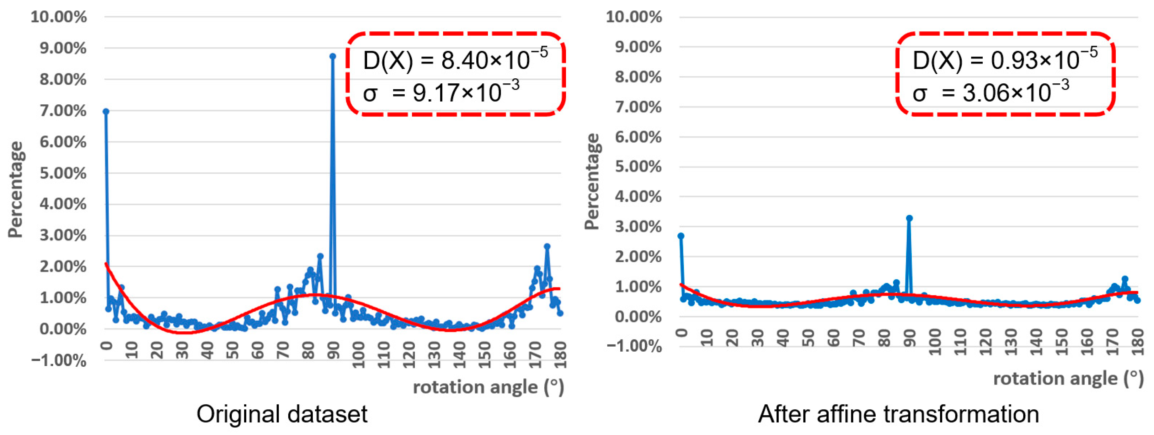
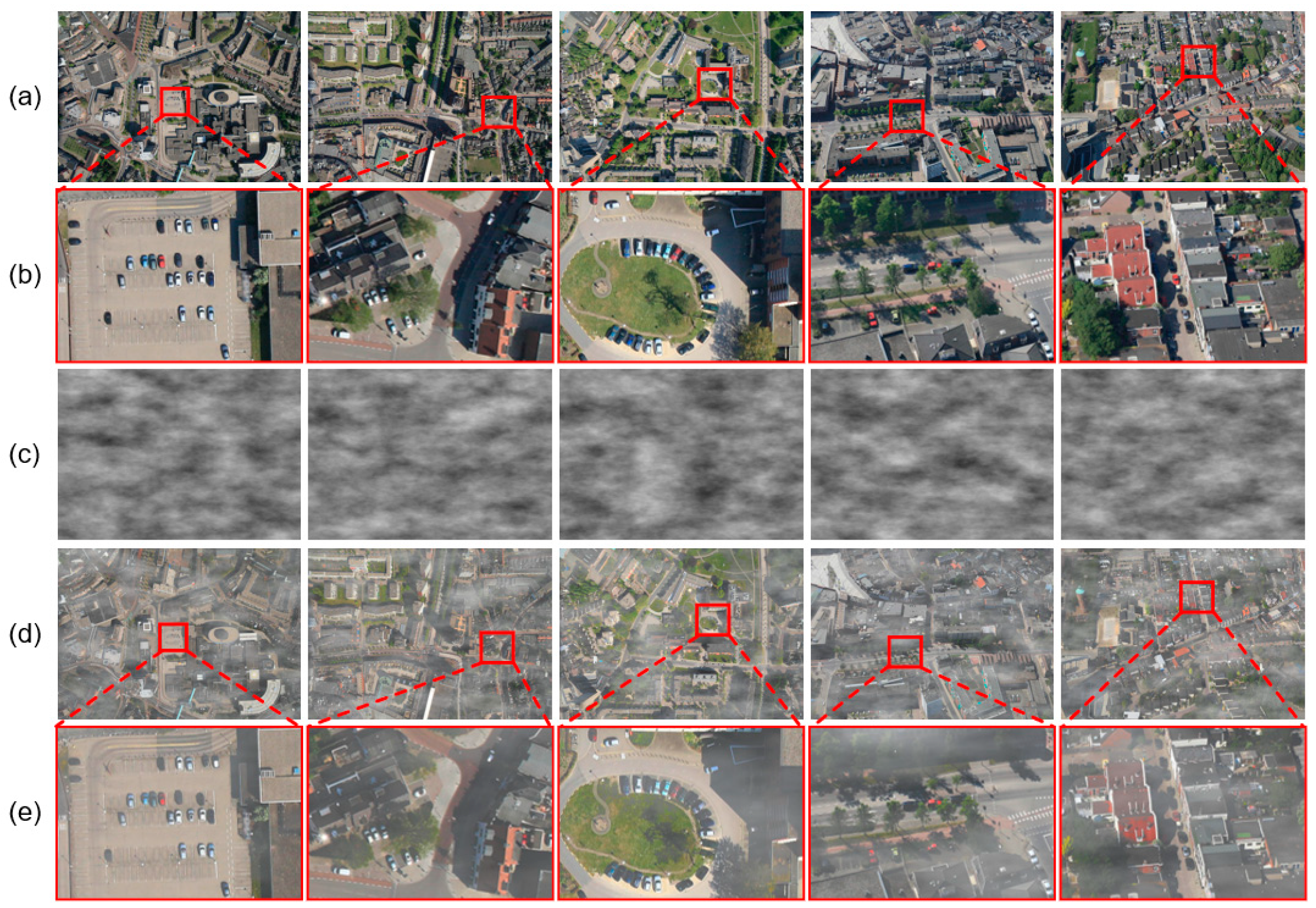
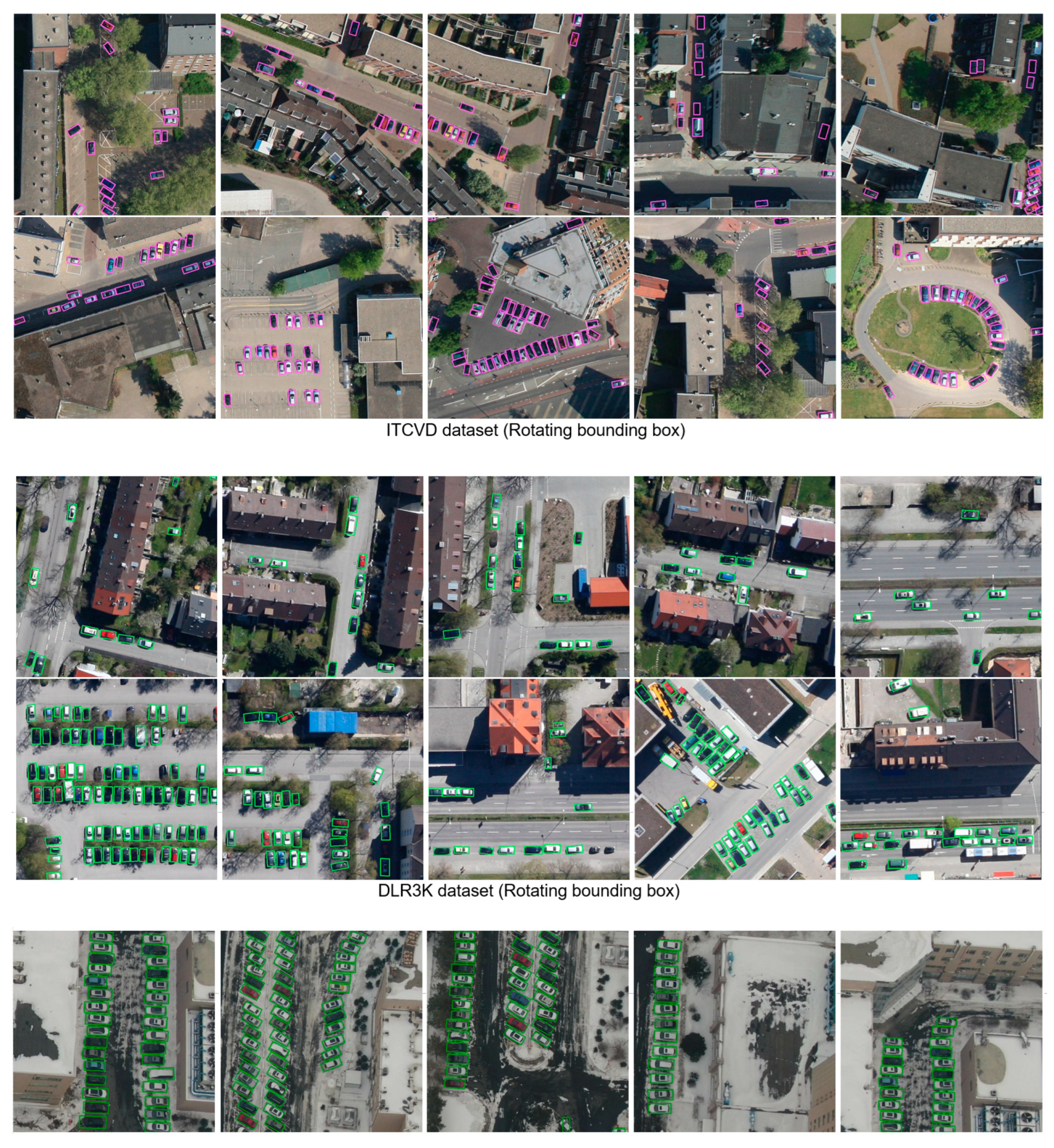
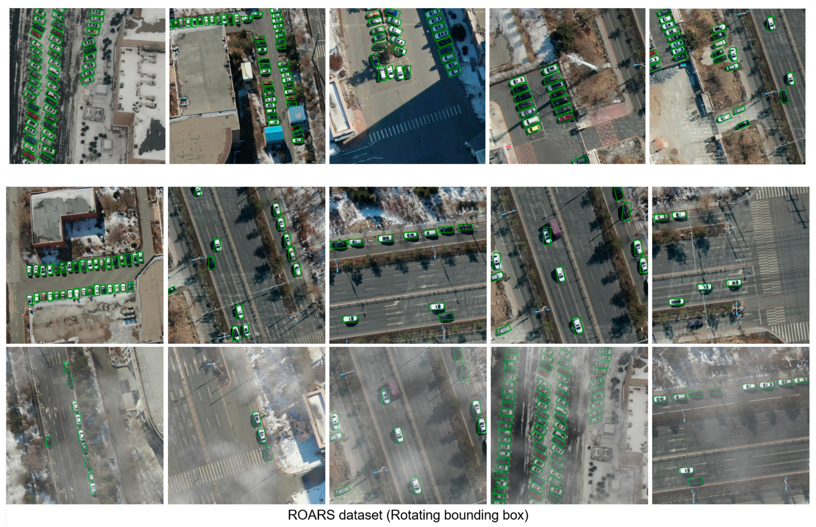
We designed an aerial remote sensing image dataset (RO-ARS) with rotating boxes. The dataset has annotated flight height and camera focal length. In order to improve the authenticity of the dataset, we propose affine transformation and haze simulation methods to augment the dataset.

The rest of this paper is organized as follows: Section 2 starts with the proposed image cutting method and then introduces the details of the proposed dataset, including the affine transformation and haze simulation methods. Furthermore, the details of the proposed SSRD-Net model are introduced. In Section 3, through several experiments, the image segmentation method, affine transformation, and haze simulation method are evaluated and discussed. Finally, the conclusions are provided in Section 4.

2. Method

The framework of our proposed vehicle detection method is illustrated in Figure 1. It is mainly composed of three parts: image pretreatment, feature extraction, and image mosaic. During image pretreatment, original large-scale images are cropped into small-scale blocks for training and testing. Through the proposed model (SSRD-Net), we will get the vehicle detection result of each block. In the end, we mosaic all the blocks together and use the non-maximum suppression [56] (NMS) method to eliminate duplicate targets. In this section, we will give the details for each part of the framework proposed, and discuss how our method improves the accuracy of vehicles detection in aerial images.

2.1. Image Segmentation

As described, putting the original image into the detection model is not suitable for aerial remote sensing images with a large field of view. If the original image is cropped with a fixed size, the target in the resulting image, which has a large-scale range, will remain unchanged. For this reason, it requires the detection model to have multi-scale target detection capabilities, which will affect the detection efficiency of the method. In order to solve the problem of inconsistent target scales in aerial remote sensing images at different flight heights and camera focal lengths, we propose an adaptive cutting method.

The above can be known by analyzing the shooting situation of aerial remote sensing images that the image shooting angle is usually close to vertical to the ground. According to the schematic diagram of the camera in Figure 1, the parameter relationship can be represented as

$$\frac{w}{v}=\frac{w_t}{h}(h>>v)$$

(1)

where w is the optical size of the target on CMOS/CCD, $w_t$ is the physical size, v is image distance and h is object distance. The basic relationship among focal length (f), object distance (h), and image distance (v) can be expressed by a Gaussian imaging equation:

$$\frac{1}{v}+\frac{1}{h}=\frac{1}{f}$$

(2)

Obviously, the object distance (h) is much larger than the image distance (v) in the aerial remote sensing image, so we conclude:

$$v=f$$

(3)

According to Formulas (1) and (3), the actual number of pixels occupied by the target can be expressed as:

$$k=\frac{w}{p}=\frac{w_t\cdot f}{h\cdot p}(h>>v)$$

(4)

where p denotes the pixel size.

It can be concluded that the number of the target pixels depends on the flight altitude and camera focal length. Accordingly, we partition images of arbitrary size into manageable cutouts with the number of target pixels. Partitioning takes place via a sliding window with overlap. The size of partitioning ($L_P$) and overlap ($L_o$) are defined as:

$$\{\begin{array}{cc}{L}_p=a\cdot k& (a=N_{gird})\\ L_o=b\cdot k& (1<b<a)\end{array}$$

(5)

where a and b are the hyperparameters. By default, a is equal to the number of output grids ($N_{gird}$) so that each grid corresponds to only one target. To avoid omissions caused by the segmentation of the target, b is set to a number greater than 1 (1.5 by default). During the mosaic process, non-maximal suppression of this overlap is necessary to refine detections at the edge of the cutouts.

2.2. Data Augmentation

According to the research status described in Section 1, the number of pictures in the aerial image data set is insufficient. It is a heavy task to construct a large number of aerial remote sensing images. To enrich the content of the dataset and improve the robustness of our model, we design a method to increase the dataset size.

Affine transformation explains the mapping between two images, which can be regarded as the superposition of linear transformation and translation transformation; it plays an important role in image correction [57,58,59], image registration [60], etc. In cartesian coordinates, it is expressed as:

$$\left[\begin{array}{l}u\hfill \\ v\hfill \end{array}\right]=A\cdot \left[\begin{array}{l}x\hfill \\ y\hfill \end{array}\right]+B=\left[\begin{array}{cc}{a}_{00}& a_{01}\\ a_{10}& a_{11}\end{array}\right]\cdot \left[\begin{array}{l}x\hfill \\ y\hfill \end{array}\right]+\left[\begin{array}{l}{b}_{00}\hfill \\ b_{10}\hfill \end{array}\right]$$

(6)

where $\left(x,y\right)$ is the original pixel point coordinates, $\left(u,v\right)$ is the point coordinates after an affine transformation. Its basic transformations as shown in Figure 2, include: translation, scale, rotation, reflection and shear. Notably, aerial remote sensing images can be rotated at any angle and the scale is limited (0.8–1.2 by default).

Moreover, to solve the problem of complex cloud and fog weather in aerial images, we propose an image degradation method in the cloudy interference state. Retinex (Retina Cortex) theory [51,52] points out that the observable information of an object is determined by two factors: the reflection properties of the object and the light intensity around the object. The light intensity determines the dynamic range of all pixels in the original image, and the inherent property (color) of the original image is determined by the reflection coefficient of the object.

As shown in the left of Figure 3, the object is illuminated by global atmospheric light, and then the light is reflected to form an image. The process can be expressed as:

$$\mathrm{I}(x)=\mathrm{J}(x)\mathrm{t}(x)+\mathrm{A}(1-\mathrm{t}(x))$$

(7)

where $\mathrm{I}\left(x\right)$ is the observed intensity, A is the global atmospheric light, $\mathrm{J}\left(x\right)$ is the scene radiance, and $\mathrm{t}\left(x\right)$ is the medium transmission and describes the portion of the light that is not scattered and reaches the camera.

The goal of haze simulation is to create A and $\mathrm{t}\left(x\right)$, we only need to add global atmospheric light noise to the original image. The noise can be considered as a random process, we use Perlin Noise [61,62] and Fractal Brownian Motion [63,64] to simulate it.

As shown in Figure 3, we define a lattice structure, each vertex of the lattice has a random gradient vector ($\overrightarrow{a_{00}},\overrightarrow{a_{01}},\overrightarrow{a_{10}},\overrightarrow{a_{11}}$ in Figure 3); therefore, each coordinate in the noise map is surrounded by four vertices. The dot product of the distance vector and the gradient vector is defined as:

$$g_{ij}=\overrightarrow{a_{ij}}·\left[\begin{array}{l}u-i\hfill \\ v-j\hfill \end{array}\right](i=1,2;j=1,2)$$

(8)

where $a_{ij}$ is the gradient vector of each corresponding corner, $\left[u-i.v-j\right]$ is the distance vector between the target point and each corresponding vertex; thus, the noise at this point can be defined as:

$$k_0=g_{00}(1-\mathrm{s}(u))+g_{01}\mathrm{s}(u)$$

(9)

$$k_1=g_{10}(1-\mathrm{s}(u))+g_{11}\mathrm{s}(u)$$

(10)

$$n=k_0(1-\mathrm{s}(v))+k_1\mathrm{s}(v)$$

(11)

where $\mathrm{s}\left(t\right)$ is the weight function, and it needs to meet the following requirements:

$$\mathrm{s}(0)=0and\mathrm{s}(0.5)=0.5and\mathrm{s}(1)=1$$

(12)

To make the noise more natural, the first and second derivatives of the smoothing function we used are zero at both $t=0$ and $t=1$:

$$\mathrm{s}(t)=6t^5-15t^4+10t^3$$

(13)

Ultimately, we got the simulated noise, which is shown in Figure 3. As can be seen, the appearance of the noise is determined by the number of lattice structures. To simulate the effect of clouds and fog more realistically, we have fused different noises:

$$N={\displaystyle {\sum }_{i=0}^j{n}_i{q}^i}(j=1,2,3,\dots )$$

(14)

$$s.t.\mathrm{L}(n_0)<\mathrm{L}(n_1)<\mathrm{L}(n_2)<\dots <\mathrm{L}(n_j)$$

(15)

where q is a scaling factor (0.7 by default), and $\mathrm{L}\left(n\right)$ represents the number of lattice structures in n. Notably, the number of lattices should remain the same to ensure the additivity of noise at different scales.

2.3. The Proposed SSRD-Net

Motivated by YOLOv4 [33], our approach uses a one-stage object detection strategy. In this section, we will give the details for each of the sub-networks. We design a single-scale vehicle detector, named SSRD-Net, to simultaneously perform small-sized vehicle object localization and classification.

2.3.1. Overall Architecture

In recent years, hierarchical detection models have achieved good performance, such as Feature Pyramid Networks (FPN) [44]. Usually, these models must stack more convolutional layers to ensure the appropriateness of the receiving domain. In the detection of small-sized objects, each pixel belonging to the small-sized object has a great influence on the final detection result, and an excessively deep network structure will make the target feature submerged by environmental information. We have initially unified the target scale as described in Section 2.1, so we propose some strategies to reduce the depth of the model, increase the number of the feature channels, and remove the irrelevant structure of the model.

As shown in Figure 4, the model designed mainly consists of four parts: input, backbone, neck, and head. The input part is an RGB aerial image resized to 608 × 608 pixels. The detection backbone extracts feature of the image through a series of convolutional structures. The detection neck is a feature extraction network that combines shallow features and deep features. The detection head predicts the category of each pixel in the output heat map, the position offset of bounding boxes, and the deflection angle.

In the detection backbone, the focus structure divides the target into smaller pixel sizes; however, each pixel belonging to a small-sized object has a great influence on the final detection result, which is not friendly to small targets. Therefore, we introduce the up-sample structure before Focus to increase the channel and reduce the depth of the network.

In the detection neck, small targets can only be detected by a 76 × 76 grid, so we eliminate the 38 × 38 and 19 × 19 grid modules in the original YOLO method; this significantly reduces the computational complexity of the model and improves the detection efficiency of the network. In addition, due to the lack of effective communication between receptive fields of different sizes, these models are limited in their ability to express generated features. We introduced the global relational (GR) block to alleviate these limitations.

In the detection head, we use a detection frame with a rotation angle to detect the target, which effectively distinguishes dense targets, prevents a large amount of overlap between the detection frames, and further improves the actual detection effect.

Table 1. SSRD-Net Network Architecture.

	From	Number	Type	Output Shape	Param
/	/	/	input	[−1, 3, 608, 608]	/
0	−1	1	Upsample	[−1, 3, 1216, 1216]	-
1	−1	1	Focus	[−1, 64, 608, 608]	7040
2	−1	1	Convolution	[−1, 128, 304, 304]	73,984
3	−1	1	Convolution	[−1, 128, 152, 152]	147,712
4	−1	3	BottleneckCSP	[−1, 128, 152, 152]	161,152
5	−1	1	Convolution	[−1, 256, 76, 76]	295,424
6	−1	9	BottleneckCSP	[−1, 256, 76, 76]	1,627,904
7	−1	1	Convolution	[−1, 512, 38, 38]	1,180,672
8	−1	9	BottleneckCSP	[−1, 512, 38, 38]	6,499,840
9	−1	1	Convolution	[−1, 1024, 19, 19]	4,720,640
10	−1	1	SPP	[−1, 1024, 19, 19]	2,624,512
11	−1	3	BottleneckCSP	[−1, 1024, 19, 19]	10,234,880
12	−1	1	Convolution	[−1, 512, 19, 19]	525,312
13	−1	1	GR Block	[−1, 512, 19, 19]	1,048,576
14	−1	1	Upsample	[−1, 512, 38, 38]	-
15	[−1, 7]	1	Concat	[−1, 1024, 38, 38]	-
16	−1	1	BottleneckCSP	[−1, 512, 38, 38]	1,510,912
17	−1	1	Convolution	[−1, 256, 38, 38]	131,584
18	−1	1	GR Block	[−1, 256, 38, 38]	262,144
19	−1	1	Upsample	[−1, 256, 76, 76]	-
20	[−1, 5]	1	Concat	[−1, 512, 76, 76]	-
21	−1	1	BottleneckCSP	[−1, 256, 76, 76]	378,624
22	−1	1	Detect	[−1, 17328, 186]	143,406
388 Conv layers		3.157 × 108 gradients		103.0 GFLOPS	3.157 × 107 parameters

below is the network structure of the proposed model.

In Table 1, “from” means the input of the block, “number” means the number of repetitions, and “Param” is the parameter amount of the block. The backbone of the model adopts the CSPDarknet53 architecture, which effectively extracts the feature information of different receptive fields. The feature fusion part removes unnecessary output structures and improves the detection speed of the model.

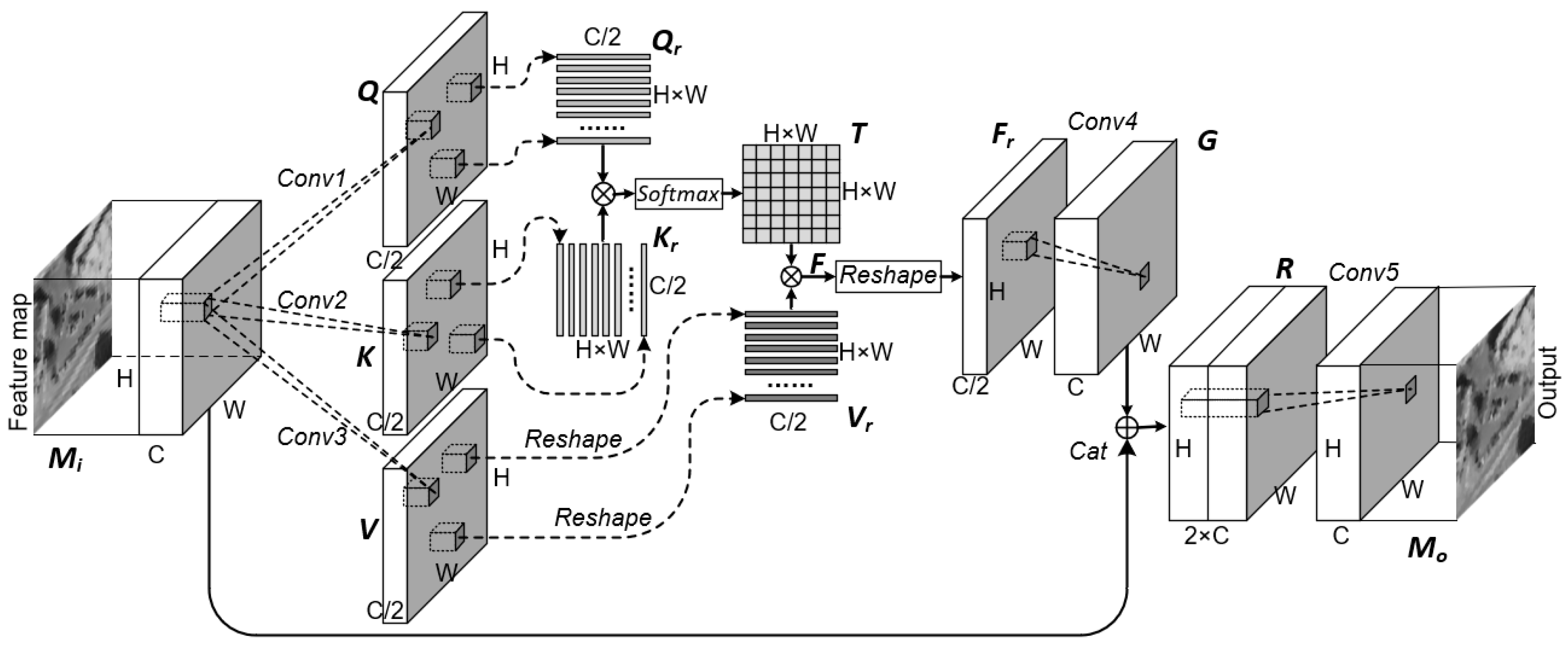
2.3.2. Global Relational Block

The location of the target in the aerial image is arbitrary. There are a large number of similar targets in the urban context. The simple connection of the convolution operator will make the network only focus on the local neighborhood, and cannot sensitively capture the global relationship among the entire spacetime. The global context-aware blocks are built in many detection tasks, via the aggregation of convolution operators in the same layer. Based on this observation, the design of the GCA block was inspired by Non-local Neural Networks [65], Double Attention Networks [66], and Compact Generalized Non-local Networks [67].

The key to the global context awareness block is that the response of a location is the weighted sum of all location features. We define global context-aware blocks in a convolutional neural network as:

$$y_i={\displaystyle \sum _{\forall j}\frac{f(x_i,x_j)}{C(x)}g(x_j)}$$

(16)

where i is the index of an output position and j is the index of all possible positions. x is the input feature map and y is the output feature map of the GR block. $f\left(x_i,x_j\right)$ represents the correlation measurement function of two points in the feature map. $g\left(x\right)$ represents the convolutional map of x. The response is normalized by a factor $C\left(x\right)$.

We define $f\left(x_i,x_j\right)$ as the similarity of the dot-product:

$$f(x_i,x_j)=\theta {(x_i)}^T\varphi (x_j)$$

(17)

where θ and ϕ are the convolutional structures to be trained, so that, there will be a pairwise connection between $x_i$ and $x_j$. We set the normalization factor as $C\left(x\right)=N$, where $N$ is the number of positions in input feature map, because it simplifies gradient computation.

In detail, as shown in Figure 5, given discriminative feature maps $M_i^{C\times H\times W}$, we transform them into a latent space ($Q^{C/2\times H\times W}$,$K^{C/2\times H\times W}$,$V^{C/2\times H\times W}$) by using different convolutional layers respectively. Then, they were reshaped to $Q_r^{HW\times C/2}$,$K_r^{C/2\times HW}$ and $V_r^{HW\times C/2}$. According to Equation (17), we can obtain a vector subset of feature vectors to capture the relationship between each subregion, $T^{HW\times HW}$ can be expressed as:

$$T^{HW\times HW}=softmax(Q_r{}^{HW\times C/2}\cdot K_r{}^{C/2\times HW})$$

(18)

The correlation matrix is defined as follows:

$$F_r{}^{C/2\times H\times W}=reshape(T^{HW\times HW}\cdot V_r{}^{HW\times C/2})$$

(19)

$G^{C\times H\times W}$ is calculated by a convolutional layer with 1 × 1 filter on $F_r$. To prevent network degradation, we define $R^{2C\times H\times W}$ as:

$$R^{2C\times H\times W}=G^{C\times H\times W}+M_i{}^{C\times H\times W}$$

(20)

Finally, we obtain the output layer $M_o^{C\times H\times W}$ through a convolutional layer with 1 × 1 filters. With the iterative update of the weight, this block can gradually extract useful context information to correct the prediction of this pixel.

The BR block enhances the discrimination of pixel features by designing a pixel-to-pixel relationship matrix. It is completely differentiable, so it can be easily optimized through backpropagation. The BR block has the same input and output dimensions, so it can be easily integrated into our detection model.

2.3.3. Prediction

Based on the regression method, we design the target detection model. As analyzed in Section 2.1 Equation (5), the size of the grid corresponds to a target. We divide the image into an S × S (76 × 76 by default) grid and each grid cell predicts some bounding boxes, confidence for those boxes, class probabilities and the rotation angle of those boxes.

As shown in Figure 6, each cell in the grid is designed with anchors centered on the cell. The output of the model includes the center coordinates of the bounding box $\left(b_x,b_y\right)$, the long-side and short-side of bounding boxes $\left(b_l,b_s\right)$, and angle $a$. We define them as:

$$b_x=\sigma (t_x)+i\cdot c_x$$

(21)

$$b_y=\sigma (t_y)+j\cdot c_y$$

(22)

$$b_l=p_l\cdot e^{t_l}$$

(23)

$$b_s=p_s\cdot e^{t_s}$$

(24)

Here $\left(i,j\right)$ is the coordinate of the corresponding grid, $\left(c_x,c_y\right)$ is the pixel size of cell, $\left[\sigma \left(t_x\right),\sigma \left(t_y\right)\right]$ is the coordinate offset of cell, $p_l$ and $p_s$ are the long-side and short-side of anchors. We consider the rotation angle as the result of classification, so each bounding box has 180 labels for angle recognition.

Compared with other methods, the non-horizontal box has one more angle dimension, and the detection box does not need to consider the target category. We design a variant of focal loss to penalize the difference between the category of each pixel output by the network and the ground truth. For the output grid $\left(\mathrm{S}\times \mathrm{S}\right)$, each cell in the grid generates B bounding box, each bounding box contains: center coordinates $\left(x,y\right)$, long-side (l), short-side (s), object confidence (c), angle (a). Object loss ($L_{obj}$) and angle loss ($L_{angle}$) are calculated by binary cross entropy (BCE). We define them as:

$$L_{obj}={\displaystyle \sum _{i=0}^{S^2}{\mathbb{I}}_{ij}^{obj}\left[{\widehat{c}}_i\ln (c_i)+\left(1-{\widehat{c}}_i\right)\ln (1-c_i)\right]}$$

(25)

$$L_{angle}={\displaystyle \sum _{i=0}^{S^2}{\displaystyle \sum _{j=0}^B{\mathbb{I}}_{ij}^{obj}}}{\displaystyle \sum _{k=0}^{180}[{\widehat{a}}_k\ln (a_k)+(1-{\widehat{a}}_k)\ln (1-a_k)]}$$

(26)

where, $\widehat{a}$ and $\widehat{c}$ is the ground true values of a, c. ${\mathbb{I}}_{ij}^{obj}$ denotes whether the object appears in the bounding box j predictor in cell i. Object loss and angle loss are considered as multi-classification problems, so the cross-entropy loss function is adopted. For the SoftMax activation function used in the model, the cross-entropy loss function can avoid the problem that the activation function enters the saturation region, and the gradient disappears in some cases.

Consider three geometric parameters: overlap area, center point distance, and aspect ratio, we use CIOU [68] to calculate the bounding box loss ($L_{box}$):

$$L_{box}=IOU-\left(\frac{{(x-\widehat{x})}^2+{(y-\widehat{y})}^2}{c^2}+\alpha v\right)$$

(27)

$$IOU=\frac{\mathrm{Area}\mathrm{of}\mathrm{Overlap}}{\mathrm{Area}\mathrm{of}\mathrm{Union}}$$

(28)

$$v=\frac{4}{{\pi }^2}{\left(\arctan \frac{\widehat{s}}{\widehat{l}}-\arctan \frac{s}{l}\right)}^2$$

(29)

$$\alpha =\frac{v}{(1-IOU)+v}$$

(30)

where ($\widehat{x},\widehat{y},\widehat{l},\widehat{s}$) is the ground true of (x, y, l, s). c is the diagonal length of the smallest enclosing box covering two boxes. $\alpha$ is the weight parameter, and the parameter $v$ represents the consistency of the aspect ratio. The CIOU loss considers the aspect ratio of the Bounding box, which improves the regression accuracy.

Finally, the total loss can be expressed as:

$$L=L_{box}+L_{obj}+L_{angle}$$

(31)

Examples of skew IoU computation are shown in Figure 7 and the optimization process is summarized in Algorithm 1.

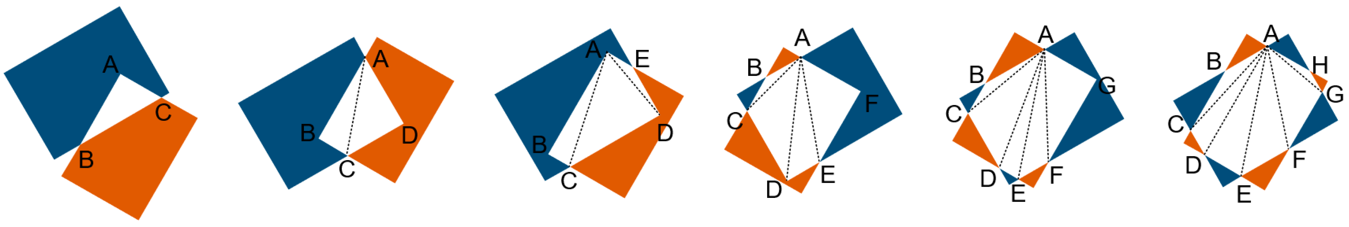
Algorithm 1 Skew IoU computation
1:	Input: Vertex coordinates of rotating bounding boxes $B_1$, $B_2$
2:	Output: IOU between rotating bounding boxes $B_1$, $B_2$
3:	Set$u\leftarrow \varnothing$, $union:S=0$
3:	Add intersection points of $B_1$ and $B_2$ to $u$
4:	Add the vertex of $B_1$ inside $B_2$ to $u$
5:	Add the vertex of $B_2$ inside $B_1$ to $u$
6:	Set $c\leftarrow$ the mean coordinates of the point in $u$
7:	Compare the coordinates of each point in $u$ and $c$, Sort $u$ into anticlockwise order
8:	Split convex polygon into $n$ triangles
9:	For each triangle ($i$) in $n$ do
10:	$S_i\leftarrow sqrt\left[p(p-a)(p-b)(p-c)\right]$ (Heron’s formula)
11:	$S\leftarrow S+S_i$
12:	End for
13:	$IOU(B_1,B_2)\leftarrow S/\left[S(B_1)+S(B_2)-S\right]$

3. Result

In this section, we discuss the setup and preprocessing of the dataset. Then, we evaluate the proposed detection method, and compare it with the state-of-the-art target detectors.

3.1. Datasets

As shown in

Table 2. Comparison of different optical remote sensing datasets.

Dataset	Images	Instances	Image Size	Source	Annotation Way	Cloud	F/H
ITCVD [40]	135	23,543	5616 × 3744	Aircraft	Horizontal	×	×
DLR 3K [50]	20	14,235	5616 × 3744	Aircraft	Horizontal	×	×
DIOR [69]	23,463	192,472	800 × 800	Google Earth	Horizontal	×	×
UCAS-AOD [70]	910	6029	~1280 × 680	Google Earth	Horizontal	×	×
DOTA [41]	2806	188,282	~2000 × 1000	Google Earth	Oriented	×	×
LEVIR [71]	22,000+	10,000+	800 × 600	Google Earth	Horizontal	×	×
HRRSD [72]	21,761	55,740	~1000 × 1000	Google Earth	Horizontal	×	×
RO-ARS	200	35,879	~2000 × 1000	Aircraft	Oriented	√	√

below, we show the comparison of different optical remote sensing datasets. Among them, F/H refers to the camera focal length and flying height.

Through comparison, it can be seen that remote sensing datasets usually have large-scale characteristics. The source images are mainly acquired from Google Earth, and most of the datasets are annotated with horizontal bounding boxes. There is no cloud phenomenon in the existing datasets, and a lack of F/H data. For the datasets above, we evaluate our method in ITCVD, DLR 3K, and our RO-ARS datasets.

3.1.1. Image Segmentation

Since ITCVD and DLR 3K lack focal length and flight height data, they cannot calculate the crop size. To verify the effectiveness of the adaptive segmentation method proposed in Section 2.1, we performed size statistics on the RO-ARS dataset. The size distributions of different cutting methods are shown in Figure 8.

Figure 8 (left) is the original width- height distribution of bounding boxes, the middle is the width-height distribution obtained by the proposed resize method. After labeling with rotating bounding box, the distribution of the long side–short side is as shown in Figure 8 (right).

The setting of anchors in target detection models depends on the target size distribution. After clustering by the Kmeans method, each color in Figure 8 represents a cluster. In analyzing the size distribution of the bounding box, we can find the rotating bounding box after resize can unify the target size better; this design makes it possible to meet the needs of the model with fewer anchors.

In addition, we also count the size and location distribution of vehicle targets, as shown in Figure 9.

It can be seen that the size of the target is relatively concentrated, and the position is evenly distributed in all positions of the picture, which can better reflect the insensitivity of the target position in the dataset.

3.1.2. Angles Distribution

Through analysis of the rotating bounding box, we count the angle distribution of the bounding box, as shown in Figure 10.

In Figure 10, $D\left(x\right)$ is the variance, σ is the standard deviation. They are defined as:

$$D(x)={\sigma }^2=\frac{{{\displaystyle \sum (x-1/180)}}^2}{180}$$

(32)

In original dataset, the rotation angle of the bounding box is 0° and 90° exceeds 20%. After affine transformation, variance and standard deviation are smaller than the original ones and the angular distribution is more even. It is helpful to improve the network’s ability to learn the target angle characteristics, and also proves the importance of affine transformation.

3.1.3. Cloud Simulation

The current aviation dataset is designed to work in sunny weather; however, bad weather, including cloud and fog, is inevitable in outdoor application. The aerial remote sensing data set must include enough complex weather images. The examples of the cloud simulation method described in Section 2.2 are shown in Figure 11.

3.2. Model Size

The proposed SSRD method is an improvement of the YOLOv5 model, we have made statistics on the parameters of the current popular target detection network, as shown in

Table 3. Parameters of neural networks for target detection.

Method	Input Shape	Anchors	Head	Parameters	Params Size (MB)
YOLOv3	3 × 608 × 608	9	3	61,949,149	236.32
YOLOv4	3 × 608 × 608	9	3	63,943,071	245.53
YOLOv5-m	3 × 608 × 608	9	3	22,229,358	84.80
YOLOv5-base	3 × 608 × 608	9	3	48,384,174	184.57
YOLOv5-x	3 × 608 × 608	9	3	89,671,790	342.07
SSD	3 × 608 × 608	9	3	23,745,908	90.58
Faster-RCNN	3 × 608 × 608	9	3	137,078,239	522.91
SSRD-base (ours)	3 × 608 × 608	3	1	31,574,318	120.45
SSRD-tiny (ours)	3 × 608 × 608	3	1	5,375,662	20.51

.

As can be seen from Table 3, the SSRD method has smaller params size compared with other models. The convolution depth of SSRD-tiny method is 0.5 times of SSRD-base, and the number of BottleneckCSP layers is 1/3 times that of SSRD-base. Some application scenarios have strict restrictions on the size of the model, such as embedded devices. The params size is positively related to the size of the output model and the small and dedicated model will have great advantages.

3.3. Evaluation Metrics

To verify the effectiveness of our proposed method, we conduct a qualitative and quantitative comparison among the current popular target detectors. The metrics of recall/precision rate, F1-score and average precision (AP) are used, which are formally defined as:

$$\mathrm{Recall}=\frac{\mathrm{number}\mathrm{of}\mathrm{true}\mathrm{detections}}{\mathrm{number}\mathrm{of}\mathrm{existing}\mathrm{objects}}=\frac{TP}{TP+FN}$$

(33)

$$\mathrm{Precision}=\frac{\mathrm{number}\mathrm{of}\mathrm{true}\mathrm{detections}}{\mathrm{number}\mathrm{of}\mathrm{detected}\mathrm{objects}}=\frac{TP}{TP+FP}$$

(34)

$$\mathrm{F}1=2\times \frac{\mathrm{Precision}\times \mathrm{Recall}}{\mathrm{Precision}+\mathrm{Recall}}$$

(35)

The area under the Precision(P)-Recall(R) curve is defined as AP. Since it is relatively difficult to calculate the integral, the interpolation method is introduced. The formula for calculating AP is defined as follows:

$$AP={\displaystyle \sum _{k=1}^N{\max }_{\tilde{k}\ge k}}P(\tilde{k})\Delta R(k)$$

(36)

The proposed method was tested and evaluated on a computer with an Intel Core i7-10700F 2.90 GHz CPU, 16 GB computer memory, and GeForce GTX 2060Ti GPU with 6 GB memory, implemented using the open-source Pytorch framework.

During the training, stochastic gradient descent [73] (SGD) is used to optimize the parameters and the basic learning rate is 1 × 10⁻⁴ The weights are initialized with Kaiming distribution [74]. The IoU threshold of non-maximum suppression (NMS) is 0.65 for inference.

3.4. Ablation Experiments

Since the RO-ARS dataset proposed contains a large number of images with cloud and fog, we test the SSRD method on ITCVD and DLR 3K datasets which have no cloud and fog image to illustrate the necessity of the cloud simulation method proposed.

The ITCVD and DLR 3K datasets lack the relevant parameters and cannot calculate the split size by the method described in Section 2.1. To fit the design of the SSRD model, we calculated the median size ($s_m$) of each image in the dataset, and then substituting $k=s_m$ into Equation (5). After cropping the image according to the calculated value, we resize them to the input size (608 × 608) of the model. Finally, we can get a dataset with a uniform target scale.

The simulation results of cloud and fog are calculated for each image in this experiment and they are shown in

Table 4. Cloud simulation performance (SSRD-base).

Dataset	Train (Cloud)	Test (Cloud)	Precision	Recall	F1	[email protected]	[email protected]:0.95
ITCVD	×	×	63.64%	75.73%	0.6916	73.78%	35.34%
ITCVD	×	√	57.34%	54.34%	0.5580	53.32%	20.45%
ITCVD	√	√	62.55%	70.27%	0.6619	71.32%	33.72%
DLR 3K	×	×	72.56%	84.34%	0.7801	78.89%	43.23%
DLR 3K	×	√	64.32%	59.23%	0.6167	60.08%	35.08%
DLR 3K	√	√	70.32%	78.89%	0.7436	75.23%	41.87%

.

It can be seen that when the training dataset lacks cloud and fog images, the model has poor performance under foggy conditions.

Adding a proper proportion of the simulation images with cloud and fog during the training will enhance the robustness of the model. The result reflects the importance of cloud and fog simulation. The ITCVD and DLR 3K datasets lack a complex meteorological environment, it is difficult to adapt to the detection tasks in real complex environments; this also provides a theoretical basis for adding complex weather images to the RO-ARS dataset.

Finally, we analyze the results obtained by training the model with different strategies and the results are shown in

Table 5. Comparison of different network methods on RO-ARS (Rotating bounding boxes).

Method	Backbone	Epoch	Precision	Recall	F1	[email protected]	[email protected]:0.95	Time (Blocks)
HOG + SVM	/	/	6.52%	21.19%	0.0997	/	/	1.3 fps
SSD300	VGG16	/	25.55%	47.34%	0.3318	24.46%	12.45%	45.5 fps
Faster-RCNN	ResNet	/	39.18%	57.36%	0.4656	39.21%	16.34%	7.2 fps
YOLOv3	Darknet53	/	21.18%	68.65%	0.3237	53.34%	20.34%	51.3 fps
YOLOv4	CSPDarknet53	/	39.72%	79.25%	0.5291	65.31%	25.38%	56.4 fps
YOLOv5s	CSPDarknet53	100	27.18%	77.52%	0.4025	58.54%	21.18%	71.4 fps
		200	34.28%	80.96%	0.4817	68.99%	27.20%
YOLOv5m	CSPDarknet53	100	26.44%	81.96%	0.3998	64.11%	24.67%	62.1 fps
		200	36.82%	79.68%	0.5036	68.56%	28.36%
YOLOv5-base	CSPDarknet53	100	32.23%	77.53%	0.4555	55.37%	23.09%	48.5 fps
		200	40.11%	73.21%	0.5182	60.33%	23.54%
YOLOv5x	CSPDarknet53	40	17.68%	81.31%	0.2904	53.34%	20.02%	30.7 fps
		100	17.54%	81.06%	0.2883	26.67%	10.28%
		150	26.35%	78.66%	0.3948	40.10%	16.11%
		200	33.29%	77.59%	0.4659	48.25%	20.09%
SSRD-base (No up-sample & GR block)	CSPDarknet53	100	40.06%	75.12%	0.5225	62.92%	23.63%	61.5 fps
		200	44.54%	76.50%	0.5630	65.70%	26.39%
SSRD-base (No up-sample)	CSPDarknet53	100	42.23%	75.69%	0.5421	65.22%	26.60%	57.8 fps
		200	56.74%	72.74%	0.6375	69.04%	29.31%
SSRD-base (No GR block)	CSPDarknet53	100	48.68%	71.67%	0.5798	65.77%	26.93%	54.9 fps
		200	57.49%	64.48%	0.6078	65.90%	28.06%
SSRD-base (ours)	CSPDarknet53	100	51.76%	76.80%	0.6184	68.29%	30.57%	49.6 fps
		200	62.52%	72.70%	0.6722	72.23%	31.69%
SSRD-tiny (ours)	CSPDarknet53	100	41.44%	76.24%	0.5369	65.36%	25.42%	92.6 fps
		200	51.62%	76.43%	0.6152	70.30%	27.78%

. Since the size of the picture segmentation depends on the relevant parameters, the number of blocks obtained is not all the same, the detection frame rate of the block will be more reliable.

The proposed model achieves a high level of detection speed and detection accuracy. The following conclusions can be verified through the experimental data of Table 5:

First, comparing SSRD-base and SSRD-base (No GR block), the precision has increased by 5.03%, F1 has increased by 0.0644, [email protected] has increased by 6.33%, and [email protected]:0.95 has increased by 3.63%; this proves the effectiveness of the GR block we proposed. Comparing SSRD-base and SSRD-base (No up-sample), the up-sample block increases the [email protected] by 3.19%, [email protected]:0.95 by 2.38%. Experiments show that the proposed up-sample block is beneficial.

Second, the small targets in complex backgrounds are difficult to detect by traditional methods (HOG + SVM). Compared with other neural networks, better results are achieved by our algorithm. The precision of the YOLO and SSD models is insufficient, and there are a large number of false detection in the results, while the detection speed of the Faster-RCNN model is slow, which is difficult to meet the requirements of practical applications.

Finally, we show some detection results of our proposed method on different datasets (ITCVD, DLR 3K, RO-ARS), as shown in Figure 12.

4. Discussion

In this work, we propose a new type of remote sensing vehicle dataset RO-ARS, which not only considers the angular distribution of the rotating bounding box, but also the diversity of the meteorological environment is considered; moreover, we use affine transformation to enhance the robustness of the model and design a cloud simulation method to increase the proportion of the images with cloud and fog; we also analyze the vehicle detection characteristics of aerial remote sensing images, and design an adaptive high-resolution image cropping scheme to improve the detection speed.

Inspired by the impressive performance of YOLOv5 in target detection, we propose a vehicle detection model suitable for aerial remote sensing images in a complex urban background. The experimental results demonstrate that the SSRD method we proposed can achieve the highest scores on [email protected] (72.23%), [email protected]:0.95 (31.69%) and F1-score (0.6722) with real-time detection speed (49.6 fps). In this work, we propose a GR block and conduct a quantitative evaluation through the ablation experiments, which proves that the GR block has excellent performance in improving the precision and reducing the false detection.

In Section 3, we analyze the relationship between the depth of the network and detection ability. The shallow neural network has a higher recall and frame, but the poor precision makes it difficult to show better performance on AP and F1. YOLOv5x with a deeper network shows a poor effect on small targets, which proves that increasing the network depth cannot solve the problem of vehicle detection in aerial remote sensing images.

5. Conclusions

The model proposed in this paper provides a feasible solution for vehicle detection in aerial remote sensing. Experiments show that the proposed model has excellent performance. The image segmentation method and cloud simulation method have a positive significance for target recognition; however, the types of cloud simulations are still not abundant. To enhance the practicality of the model, improving the detection speed is still an important research direction.

In the future, we will further improve our research topics in several aspects, such as feature extraction and fusion, the diversification of cloud simulation and model compression. Using unsupervised or weakly supervised models to reduce the model’s dependence on datasets is also one of the important design directions.

References

1. Hsieh, M.R.; Lin, Y.L.; Hsu, W.H. Drone-Based Object Counting by Spatially Regularized Regional Proposal Network. In Proceedings of the 2017 IEEE International Conference on Computer Vision (ICCV), Venice, Italy, 22–29 October 2017; pp. 4165–4173. [Google Scholar]
2. Liao, W.; Chen, X.; Yang, J.F.; Roth, S.; Goesele, M.; Yang, M.Y.; Rosenhahn, B. LR-CNN: Local-aware Region CNN for Vehicle Detection in Aerial Imagery. In Proceedings of the ISPRS Annals of Photogrammetry, Remote Sensing and Spatial Information Sciences, Nice, France, 31 August–2 September 2020; pp. 381–388. [Google Scholar]
3. Ferreira de Carvalho, O.L.; Abílio de Carvalho, O.; Olino de Albuquerque, A.; Castro Santana, N.; Leandro Borges, D.; Trancoso Gomes, R.; Fontes Guimarães, R. Bounding Box-Free Instance Segmentation Using Semi-Supervised Learning for Generating a City-Scale Vehicle Dataset. arXiv 2021, arXiv:2111.12122. [Google Scholar]
4. Deng, Z.P.; Sun, H.; Zhou, S.L.; Zhao, J.P.; Zou, H.X. Toward Fast and Accurate Vehicle Detection in Aerial Images Using Coupled Region-Based Convolutional Neural Networks. IEEE J. Sel. Top. Appl. Earth Obs. Remote Sens. 2017, 10, 3652–3664. [Google Scholar] [CrossRef]
5. Tang, T.Y.; Zhou, S.L.; Deng, Z.P.; Zou, H.X.; Lei, L. Vehicle Detection in Aerial Images Based on Region Convolutional Neural Networks and Hard Negative Example Mining. Sensors 2017, 17, 336. [Google Scholar] [CrossRef] [PubMed] [Green Version]
6. Long, Y.; Gong, Y.P.; Xiao, Z.F.; Liu, Q. Accurate Object Localization in Remote Sensing Images Based on Convolutional Neural Networks. IEEE Trans. Geosci. Remote Sens. 2017, 55, 2486–2498. [Google Scholar] [CrossRef]
7. Xu, Y.Z.; Yu, G.Z.; Wang, Y.P.; Wu, X.K.; Ma, Y.L. Car Detection from Low-Altitude UAV Imagery with the Faster R-CNN. J. Adv. Transp. 2017, 2017. [Google Scholar] [CrossRef] [Green Version]
8. Zou, Z.X.; Shi, Z.W.; Guo, Y.H.; Ye, J.P. Object Detection in 20 Years: A Survey. arXiv 2019, arXiv:1905.05055. [Google Scholar]
9. Viola, P.; Jones, M. Rapid object detection using a boosted cascade of simple features. In Proceedings of the IEEE Conference on Computer Vision and Pattern Recognition (CVPR), Kauai, America, 8–14 December 2001; pp. 511–518. [Google Scholar]
10. Viola, P.; Jones, M.J. Robust real-time face detection. Int. J. Comput. Vis. 2004, 57, 137–154. [Google Scholar] [CrossRef]
11. Dalal, N.; Triggs, B. Histograms of oriented gradients for human detection. In Proceedings of the IEEE Conference on Computer Vision and Pattern Recognition (CVPR), San Diego, CA, USA, 20–25 June 2005; pp. 886–893. [Google Scholar]
12. Felzenszwalb, P.; McAllester, D.; Ramanan, D. A discriminatively trained, multiscale, deformable part model. In Proceedings of the IEEE Conference on Computer Vision and Pattern Recognition (CVPR), Anchorage, AK, USA, 23–28 June 2008; pp. 1–8. [Google Scholar]
13. Felzenszwalb, P.F.; Girshick, R.B.; McAllester, D. Cascade Object Detection with Deformable Part Models. In Proceedings of the IEEE Conference on Computer Vision and Pattern Recognition (CVPR), San Francisco, CA, USA, 13–18 June 2010; pp. 2241–2248. [Google Scholar]
14. Felzenszwalb, P.F.; Girshick, R.B.; McAllester, D.; Ramanan, D. Object Detection with Discriminatively Trained Part-Based Models. IEEE Trans. Pattern Anal. Mach. Intell. 2010, 32, 1627–1645. [Google Scholar] [CrossRef] [PubMed] [Green Version]
15. Girshick, R.B.; Felzenszwalb, P.F.; McAllester, D. Object Detection with Grammar Models. In Proceedings of the International Conference on Neural Information Processing Systems, Granada, Spain, 12–17 December 2011; pp. 442–450. [Google Scholar]
16. Wang, S. Vehicle detection on Aerial Images by Extracting Corner Features for Rotational Invariant Shape Matching. In Proceedings of the IEEE 11th International Conference on Computer and Information Technology (CIT), Paphos, Cyprus, 31 August–2 September 2011; pp. 171–175. [Google Scholar]
17. Szegedy, C.; Liu, W.; Jia, Y.Q.; Sermanet, P.; Reed, S.; Anguelov, D.; Erhan, D.; Vanhoucke, V.; Rabinovich, A. Going Deeper with Convolutions. In Proceedings of the IEEE Conference on Computer Vision and Pattern Recognition (CVPR), Boston, MA, USA, 7–12 June 2015; pp. 1–9. [Google Scholar]
18. Krizhevsky, A.; Sutskever, I.; Hinton, G.E. ImageNet Classification with Deep Convolutional Neural Networks. Commun. ACM 2017, 60, 84–90. [Google Scholar] [CrossRef]
19. Everingham, M.; Eslami, S.M.A.; Van Gool, L.; Williams, C.K.I.; Winn, J.; Zisserman, A. The PASCAL Visual Object Classes Challenge: A Retrospective. Int. J. Comput. Vis. 2015, 111, 98–136. [Google Scholar] [CrossRef]
20. Everingham, M.; Van Gool, L.; Williams, C.K.I.; Winn, J.; Zisserman, A. The Pascal Visual Object Classes (VOC) Challenge. Int. J. Comput. Vis. 2010, 88, 303–338. [Google Scholar] [CrossRef] [Green Version]
21. Gupta, A.; Dollar, P.; Girshick, R. LVIS: A Dataset for Large Vocabulary Instance Segmentation. In Proceedings of the IEEE Conference on Computer Vision and Pattern Recognition (CVPR), Long Beach, CA, USA, 16–20 June 2019; pp. 5351–5359. [Google Scholar]
22. Lin, T.Y.; Maire, M.; Belongie, S.; Hays, J.; Perona, P.; Ramanan, D.; Dollar, P.; Zitnick, C.L. Microsoft COCO: Common Ob-jects in Context. In Proceedings of the European Conference on Computer Vision (ECCV), Zurich, Switzerland, 6–12 September 2014; pp. 740–755. [Google Scholar]
23. Zuo, C.; Qian, J.; Feng, S.; Yin, W.; Li, Y.; Fan, P.; Han, J.; Qian, K.; Chen, Q. Deep learning in optical metrology: A review. Light Sci. Appl. 2022, 11, 39. [Google Scholar] [CrossRef] [PubMed]
24. Li, X.; Zhang, G.; Qiao, H.; Bao, F.; Deng, Y.; Wu, J.; He, Y.; Yun, J.; Lin, X.; Xie, H.; et al. Unsupervised content-preserving transformation for optical microscopy. Light Sci. Appl. 2021, 10, 44. [Google Scholar] [CrossRef] [PubMed]
25. Huang, L.; Luo, R.; Liu, X. Spectral imaging with deep learning. Light Sci. Appl. 2022, 11, 61. [Google Scholar] [CrossRef]
26. Zhang, Y.; Liu, T.; Singh, M.; Cetintas, E.; Luo, Y.; Rivenson, Y.; Larin, K.V.; Ozcan, A. Neural network-based image reconstruction in swept-source optical coherence tomography using undersampled spectral data. Light Sci. Appl. 2021, 10, 155. [Google Scholar] [CrossRef]
27. Dai, J.F.; Li, Y.; He, K.M.; Sun, J. R-FCN: Object Detection via Region-based Fully Convolutional Networks. In Proceedings of the Conference on Neural Information Processing Systems (NIPS), Barcelona, Spain, 5–10 December 2016. [Google Scholar]
28. Ren, S.Q.; He, K.M.; Girshick, R.; Sun, J. Faster R-CNN: Towards Real-Time Object Detection with Region Proposal Networks. IEEE Trans. Pattern Anal. Mach. Intell. 2017, 39, 1137–1149. [Google Scholar] [CrossRef] [PubMed] [Green Version]
29. Girshick, R.; Donahue, J.; Darrell, T.; Malik, J. Rich feature hierarchies for accurate object detection and semantic segmentation. In Proceedings of the IEEE Conference on Computer Vision and Pattern Recognition (CVPR), Columbus, OH, USA, 23–28 June 2014; pp. 580–587. [Google Scholar]
30. Redmon, J.; Divvala, S.; Girshick, R.; Farhadi, A. You Only Look Once: Unified, Real-Time Object Detection. In Proceedings of the IEEE Conference on Computer Vision and Pattern Recognition (CVPR), Seattle, WA, USA, 27–30 June 2016; pp. 779–788. [Google Scholar]
31. Redmon, J.; Farhadi, A. YOLO9000: Better, Faster, Stronger. In Proceedings of the IEEE/CVF Conference on Computer Vision and Pattern Recognition (CVPR), Honolulu, HI, USA, 21–26 July 2017; pp. 6517–6525. [Google Scholar]
32. Redmon, J.; Farhadi, A. YOLOv3: An Incremental Improvement. arXiv 2018, arXiv:1804.02767. [Google Scholar]
33. Bochkovskiy, A.; Wang, C.Y.; Liao, H. YOLOv4: Optimal Speed and Accuracy of Object Detection. arXiv 2020, arXiv:2004.10934. [Google Scholar]
34. Liu, W.; Anguelov, D.; Erhan, D.; Szegedy, C.; Reed, S.; Fu, C.Y.; Berg, A.C. SSD: Single Shot MultiBox Detector. In Proceedings of the 14th European Conference on Computer Vision (ECCV), Amsterdam, The Netherlands, 8–16 October 2016; pp. 21–37. [Google Scholar]
35. Tay, Y.; Dehghani, M.; Bahri, D.; Metzler, D. Efficient Transformers: A Survey. arXiv 2020, arXiv:2009.06732. [Google Scholar] [CrossRef]
36. Han, K.; Wang, Y.H.; Chen, H.T.; Chen, X.H.; Guo, J.Y.; Liu, Z.H.; Tang, Y.H.; Xiao, A.; Xu, C.J.; Xu, Y.X.; et al. A Survey on Vision Transformer. arXiv 2020, arXiv:2012.12556. [Google Scholar] [CrossRef]
37. Khan, S.; Naseer, M.; Hayat, M.; Waqas Zamir, S.; Shahbaz Khan, F.; Shah, M. Transformers in Vision: A Survey. arXiv 2021, arXiv:2101.01169. [Google Scholar] [CrossRef]
38. Carion, N.; Massa, F.; Synnaeve, G.; Usunier, N.; Kirillov, A.; Zagoruyko, S. End-to-End Object Detection with Transformers. arXiv 2020, arXiv:2005.12872. [Google Scholar]
39. Dai, J.F.; Qi, H.Z.; Xiong, Y.W.; Li, Y.; Zhang, G.D.; Hu, H.; Wei, Y.C. Deformable Convolutional Networks. In Proceedings of the IEEE International Conference on Computer Vision (ICCV), Venice, Italy, 22–29 October 2017; pp. 764–773. [Google Scholar]
40. Yang, M.Y.; Liao, W.T.; Li, X.B.; Cao, Y.P.; Rosenhahn, B. Vehicle Detection in Aerial Images. Photogramm. Eng. Remote Sens. 2019, 85, 297–304. [Google Scholar] [CrossRef] [Green Version]
41. Xia, G.S.; Bai, X.; Ding, J.; Zhu, Z.; Belongie, S.; Luo, J.B.; Datcu, M.; Pelillo, M.; Zhang, L.P. DOTA: A Large-scale Dataset for Object Detection in Aerial Images. In Proceedings of the IEEE Conference on Computer Vision and Pattern Recognition (CVPR), Salt Lake City, GA, USA, 18–23 June 2018; pp. 3974–3983. [Google Scholar]
42. Van Etten, A. You Only Look Twice: Rapid Multi-Scale Object Detection In Satellite Imagery. arXiv 2018, arXiv:1805.09512. [Google Scholar]
43. He, K.M.; Gkioxari, G.; Dollár, P.; Girshick, R. Mask R-CNN. In Proceedings of the IEEE International Conference on Computer Vision (ICCV), Venice, Italy, 22–29 October 2017; pp. 2980–2988. [Google Scholar]
44. Lin, T.Y.; Dollar, P.; Girshick, R.; He, K.M.; Hariharan, B.; Belongie, S. Feature Pyramid Networks for Object Detection. In Proceedings of the IEEE /CVF Conference on Computer Vision and Pattern Recognition (CVPR), Honolulu, GA, USA, 21–26 July 2017; pp. 936–944. [Google Scholar]
45. Li, J.N.; Wei, Y.C.; Liang, X.D.; Dong, J.; Xu, T.F.; Feng, J.S.; Yan, S.C. Attentive Contexts for Object Detection. IEEE Trans. Multimed. 2017, 19, 944–954. [Google Scholar] [CrossRef] [Green Version]
46. Chen, X.L.; Gupta, A. Spatial Memory for Context Reasoning in Object Detection. In Proceedings of the IEEE International Conference on Computer Vision (ICCV), Venice, Italy, 22–29 October 2017; pp. 4106–4116. [Google Scholar]
47. Cao, J.X.; Chen, Q.; Guo, J.; Shi, R.C. Attention-guided Context Feature Pyramid Network for Object Detection. arXiv 2020, arXiv:2005.11475. [Google Scholar]
48. Lim, J.S.; Astrid, M.; Yoon, H.J.; Lee, S.I. Small Object Detection using Context and Attention. In Proceedings of the International Conference on Artificial Intelligence in Information and Communication (IEEE ICAIIC), Jeju Island, Korea, 13–16 April 2021; pp. 181–186. [Google Scholar]
49. Razakarivony, S.; Jurie, F. Vehicle detection in aerial imagery: A small target detection benchmark. J. Vis. Commun. Image Represent 2016, 34, 187–203. [Google Scholar] [CrossRef] [Green Version]
50. Liu, K.; Mattyus, G. Fast Multiclass Vehicle Detection on Aerial Images. IEEE Geosci. Remote. Sens. Lett. 2015, 12, 1938–1942. [Google Scholar]
51. He, K.M.; Sun, J.; Tang, X.O. Single Image Haze Removal Using Dark Channel Prior. IEEE Trans. Pattern Anal. Mach. Intell. 2011, 33, 2341–2353. [Google Scholar]
52. Hsieh, C.H.; Zhao, Q.F.; Cheng, W.C. Single Image Haze Removal Using Weak Dark Channel Prior. In Proceedings of the International Conference on Awareness Science and Technology (iCAST), Fukuoka, Japan, 19–21 September 2018; pp. 214–219. [Google Scholar]
53. Tan, R.T. Visibility in bad weather from a single image. In Proceedings of the IEEE Conference on Computer Vision and Pattern Recognition (CVPR), Anchorage, AK, USA, 23–28 June 2008; pp. 2347–2354. [Google Scholar]
54. Zhu, Q.S.; Mai, J.M.; Shao, L. A Fast Single Image Haze Removal Algorithm Using Color Attenuation Prior. IEEE Trans. Image Process. 2015, 24, 3522–3533. [Google Scholar]
55. Cai, B.L.; Xu, X.M.; Jia, K.; Qing, C.M.; Tao, D.C. DehazeNet: An End-to-End System for Single Image Haze Removal. IEEE Trans. Image Process. 2016, 25, 5187–5198. [Google Scholar] [CrossRef] [PubMed] [Green Version]
56. Zheng, Z.H.; Wang, P.; Liu, W.; Li, J.Z.; Ye, R.G.; Ren, D.W. Distance-IoU Loss: Faster and Better Learning for Bounding Box Regression. In Proceedings of the AAAI Conference on Artificial Intelligence, New York, NY, USA, 7–12 February 2020; pp. 12993–13000. [Google Scholar]
57. Jaderberg, M.; Simonyan, K.; Zisserman, A.; Kavukcuoglu, K. Spatial Transformer Networks. In Proceedings of the Annual Conference on Neural Information Processing Systems (NIPS), Montreal, QC, Canada, 7–12 December 2015. [Google Scholar]
58. Hinton, G.E.; Krizhevsky, A.; Wang, S.D. Transforming Auto-Encoders. In Proceedings of the International Conference on Artificial Neural Networks (ICANN), Espoo, Finland, 14–17 June 2011; pp. 44–51. [Google Scholar]
59. Yip, B. Face and eye rectification in video conference using affine transform. In Proceedings of the IEEE International Conference on Image Processing (ICIP), Genoa, Italy, 11–14 September 2005; pp. 3021–3024. [Google Scholar]
60. Lowe, D.G. Object recognition from local scale-invariant features. In Proceedings of the IEEE International Conference on Computer Vision (ICCV), Kerkyra (Corfu), Greece, 20–27 September 1999; pp. 1150–1157. [Google Scholar]
61. Perlin, K. An Image Synthesizer. SIGGRAPH Comput. Graph. 1985, 19, 287–296. [Google Scholar] [CrossRef]
62. Perlin, K. Improving noise. ACM Trans. Graph. 2002, 21, 681–682. [Google Scholar] [CrossRef]
63. Fulinski, A. Fractional Brownian Motions. Acta Phys. Pol. B Proc. Suppl. 2020, 51, 1097–1129. [Google Scholar] [CrossRef]
64. Zili, M. Generalized fractional Brownian motion. Mod. Stoch. Theory Appl. 2017, 4, 15–24. [Google Scholar] [CrossRef] [Green Version]
65. Wang, X.L.; Girshick, R.; Gupta, A.; He, K.M. Non-local Neural Networks. In Proceedings of the IEEE Conference on Computer Vision and Pattern Recognition (CVPR), Salt Lake City, GA, USA, 18–23 June 2018; pp. 7794–7803. [Google Scholar]
66. Chen, Y.P.; Kalantidis, Y.; Li, J.S.; Yan, S.C.; Feng, J.S. A2-Nets: Double Attention Networks. In Proceedings of the Advances in Neural Information Processing Systems (NIPS), Montreal, QC, Canada, 2–8 December 2018. [Google Scholar]
67. Yue, K.Y.; Sun, M.; Yuan, Y.C.; Zhou, F.; Ding, E.R.; Xu, F.X. Compact Generalized Non-local Network. In Proceedings of the Conference on Neural Information Processing Systems (NIPS), Montreal, QC, Canada, 2–8 December 2018. [Google Scholar]
68. Zheng, Z.H.; Wang, P.; Ren, D.W.; Liu, W.; Ye, R.G.; Hu, Q.H.; Zuo, W.M. Enhancing Geometric Factors in Model Learning and Inference for Object Detection and Instance Segmentation. IEEE Trans. Cybern. 2021, 1–13. [Google Scholar] [CrossRef] [PubMed]
69. Li, K.; Wan, G.; Cheng, G.; Meng, L.Q.; Han, J.W. Object detection in optical remote sensing images: A survey and a new benchmark. ISPRS J. Photogramm. Remote Sens. 2020, 159, 296–307. [Google Scholar] [CrossRef]
70. Zhu, H.G.; Chen, X.G.; Dai, W.Q.; Fu, K.; Ye, Q.X.; Jiao, J.B. Orientation Robust Object Detection in Aerial Images Using Deep Convolutional Neural Network. In Proceedings of the IEEE International Conference on Image Processing (ICIP), Quebec City, QC, Canada, 27–30 September 2015; pp. 3735–3739. [Google Scholar]
71. Chen, H.; Shi, Z.W. A Spatial-Temporal Attention-Based Method and a New Dataset for Remote Sensing Image Change Detection. Remote Sens. 2020, 12, 1662. [Google Scholar] [CrossRef]
72. Lu, X.Q.; Zhang, Y.L.; Yuan, Y.; Feng, Y.C. Gated and Axis-Concentrated Localization Network for Remote Sensing Object Detection. IEEE Trans. Geosci. Remote Sens. 2020, 58, 179–192. [Google Scholar] [CrossRef]
73. Song, S.; Chaudhuri, K.; Sarwate, A.D. Stochastic gradient descent with differentially private updates. In Proceedings of the IEEE Global Conference on Signal and Information Processing (GLOBALSIP), Austin, TX, USA, 3–5 December 2013; pp. 245–248. [Google Scholar]
74. He, K.M.; Zhang, X.Y.; Ren, S.Q.; Sun, J. Delving Deep into Rectifiers: Surpassing Human-Level Performance on ImageNet Classification. In Proceedings of the IEEE International Conference on Computer Vision (ICCV), Santiago, Chile, 11–18 December 2015; pp. 1026–1034. [Google Scholar]
Figure 1. Proposed vehicle detection framework.
Remotesensing 14 02088 g001
Figure 2. Illustrations of different affine transformations matrix.
Remotesensing 14 02088 g002
Figure 3. Schematic diagram of the haze simulation process.
Remotesensing 14 02088 g003
Figure 4. Overall architecture of the SSRD-Net framework.
Remotesensing 14 02088 g004
Figure 5. A spacetime global relational block (GR).
Remotesensing 14 02088 g005
Figure 6. Bounding boxes with angle prediction.
Remotesensing 14 02088 g006
Figure 7. The Intersection over Union (IoU) of bounding boxes.
Remotesensing 14 02088 g007
Figure 8. The schematic diagram of the bounding box distribution (RO-ARS).
Remotesensing 14 02088 g008
Figure 9. The target size and position distribution (RO-ARS).
Remotesensing 14 02088 g009
Figure 10. Distribution of tilt angles (ITCVD dataset).
Remotesensing 14 02088 g010
Figure 11. Data augmentation. (ITCVD dataset) (a) optical image; (b) partial enlarged view; (c) cloud layer simulated; (d) simulated images with clouds; (e) partial enlarged view of simulated image.
Remotesensing 14 02088 g011
Figure 12. Results of SSRD-base detection methods in different datasets.
Remotesensing 14 02088 g012aRemotesensing 14 02088 g012b