Hyperspectral Monitoring Driven by Machine Learning Methods for Grassland Above-Ground Biomass

Abstract

Above-ground biomass (AGB) is a key indicator for studying grassland productivity and evaluating carbon sequestration capacity; it is also a key area of interest in hyperspectral ecological remote sensing. In this study, we use data from a typical alpine meadow in the Qinghai–Tibet Plateau during the main growing season (July–September), compare the results of various feature selection algorithms to extract an optimal subset of spectral variables, and use machine learning methods and data mining techniques to build an AGB prediction model and realize the optimal inversion of above-ground grassland biomass. The results show that the Lasso and RFE_SVM band filtering machine learning models can effectively select the global optimal feature and improve the prediction effect of the model. The analysis also compares the support vector machine (SVM), least squares regression boosting (LSB), and Gaussian process regression (GPR) AGB inversion models; our findings show that the results of the three models are similar, with the GPR machine learning model achieving the best outcomes. In addition, through the analysis of different data combinations, it is found that the accuracy of AGB inversion can be significantly improved by combining the spectral characteristics with the growing season. Finally, by constructing a machine learning interpretable model to analyze the specific role of features, it was found that the same band plays different roles in different records, and the related results can provide a scientific basis for the research of grassland resource monitoring and estimation.

1. Introduction

The Qinghai–Tibet Plateau’s alpine grasslands play a critical role in climate change and the global carbon cycle [1,2,3,4,5]. Grasslands use energy and materials from nature to maintain their own stable system structure and function [6,7], preventing soil erosion [8,9], purifying the air [10], and performing other functions [11], as well as serving as an important green barrier for the earth and a material source for livestock farming [2,10,12]. Grassland biomass contributes significantly to the carbon pool of terrestrial ecosystems, representing a carbon source in the form of organic matter [3,11,13]. The biomass of grassland areas objectively reflects their potential to sequester carbon and support animal life [14,15,16]. Thus, accurate grassland biomass assessment helps to reveal the role of grassland ecosystems in global climate change, as well as to understand the efficient use of grassland resources [17,18]. Grassland areas on the Tibetan Plateau have been severely degraded, with declining species diversity and decreasing biomass in recent years as a result of natural and anthropogenic factors [2]; thus, this region represents an important target area for understanding biomass change. The degree of grassland resources is linked to ecological security [19], which plays a key role in environmental preservation. As a result, in order to conserve grasslands, it is critical to conduct regular and detailed biomass estimations.

Traditional ground surveys have significant spatial and temporal restrictions; thus, research into the multispectral remote sensing estimation of grassland biomass has made significant progress [20,21,22,23]. Liang et al. [24] evaluated various methods for the above-ground biomass (AGB) estimation of alpine grassland vegetation using Moderate Resolution Imaging Spectroradiometer (MODIS) vegetation indices, in combination with long-term climate and grassland monitoring data; their study found that an NDVI-based AGB model performs best (R² of 46%) among all tested single-factor linear remote sensing models. Hai et al. [25] proposed a simulated spectral method to invert AGB using Sentinel-2 data and obtained an accurate AGB estimate, with R² = 0.95. Using this method, the root mean square error (RMSE) was 10.86 g/m², and the estimation accuracy (EA) was 82.84%. Sun et al. [26] used multispectral data obtained by an unmanned aerial vehicle (UAV) to analyze a representative area of Ziquan pasture on the northern side of the Tianshan Mountains in Xinjiang and selected the optimal waveband combination to study the natural grassland biomass, achieving an estimation model with an accuracy of 63%. Multispectral cameras, however, are characterized by a small number of bands and large bandwidth, making it difficult to accurately reflect subtle changes in vegetation in some sensitive bands and to achieve precise detection requirements [27,28,29,30]; in addition, there is a significant problem of “same body, different spectrum”. As a result, multispectral AGB inversion approaches frequently ignore grassland diversity and variability, such as grazing circumstances, growing seasons, grass height, cover, and other significant aspects [21,22,31]. Hyperspectral remote sensing, however, offers high waveband resolution, allowing researchers to effectively analyze complex and diverse natural grasslands [29].

Using hyperspectral remote sensing, information can be obtained quickly, over vast areas, and without loss [32,33,34].The prevalent “dimensional catastrophe”, or Hughes effect, leads to unstable parameter estimations in hyperspectral models [35,36]; therefore, selecting spectrally sensitive bands for above-ground biomass estimation is crucial for simplifying a model and improving its predictive capabilities; that is, the subset of relevant bands is obtained by solving an optimization problem based on specified evaluation criteria. In multivariate partial least squares regression (PLSR) models, Fava et al. [37] used all reflectance bands as input. Each model was evaluated using the cross-validated coefficient of determination and the root mean square error (RMSE) after being subjected to leave-one-out cross-validation. The average inaccuracy in predicting fresh biomass and fuel moisture content was 20%. Miguel et al. [38] constructed different vegetation index combinations from raw spectra and extracted spectral absorption features to construct a PLSR model for comparative analysis to obtain optimal results with an R² value of 0.939 and RMSE of g/m². In the study of Bratsch et al. [39], band regression using Lasso was applied to overcome the problem of excessive correlation among hyperspectral variables. The bulk of significant biomass–spectra associations (65%) were found in shrub groups and bands in the blue, green, and red edge wavelength portions of the spectrum at all times during the growing season. The above research found that using a feature selection approach to choose variables for modeling enhanced the model’s accuracy and robustness. In machine learning research, filtering, wrapping, and embedding approaches have been created as feature selection methods; however, different variable selection algorithms do not necessarily select the same feature variables, thus influencing model correctness [40]. The upper limit of the effect is determined by the features in most machine learning tasks, where the selection and combination of models can only approximate this upper limit indefinitely [41]. In grass spectral research, there is a lack of literature that carefully analyzes and compares the three types of feature selection algorithms. Accordingly, to provide a theoretical foundation for developing more efficient spectrum models, it is necessary to investigate combining numerous variable selection methods with diverse regression methods.

A range of results from hyperspectral studies of alpine grassland biomass has been obtained, providing a solid and reliable theoretical foundation for this type of study [42,43]. However, these studies use empirical analysis models, as the vegetation composition, structure, and natural conditions of different study sites are not consistent; there is thus also inconsistency in the data, models, and algorithms from different approaches, preventing the direct comparison and evaluation of their results [44]. This issue can be addressed by applying the concept of data mining to establish a standardized and normalized data analysis process, improve the modeling approach to fully explore the spectral information, and strictly control the analysis process to optimize the modeling results to ensure the validity and accuracy of the machine learning inversion model [45]. Regardless of the accuracy of their outputs, machine learning (ML) models are sometimes criticized as being “black boxes” whose internal logic is difficult for humans to understand [46]. Thus, a well-established maximum likelihood model can unfortunately only produce prediction results without providing significant insights—a problem known as interpretability [47]. Using interpretable tools to identify the relative importance of the input variables and how they interact with the output variables is one approach to resolving this challenge [48]. By merging some of the field survey data, in this study, we performed a spectral inversion model interpretability analysis and compared the results to develop a spectral–ecological variables–AGB mechanistic model with better physiological interpretability.

Based on these findings, there are few studies on systematic feature selection for the hyperspectral interpretation of alpine grassland with complex and diversified populations, and the use of interpretable machine learning in alpine grassland hyperspectral research is rarely reported. As a result, in this study, we investigated an alpine grassland experimental site in Henan County, Qinghai Province, where a fence closure experiment was designed to (i) measure the canopy spectra and ecological parameters of each typical community and carry out a statistical analysis, (ii) analyze and compare the results of different feature selection algorithms, (iii) establish an AGB estimation model using support vector machine, Gaussian process regression, least squares regression boosting, and artificial neural network, and (iv) build machine learning interpretable models to analyze the results. Overall, this study introduces a novel analytical modeling approach for monitoring above-ground biomass on the Tibetan Plateau using hyperspectral remote sensing.

2. Materials and Methods

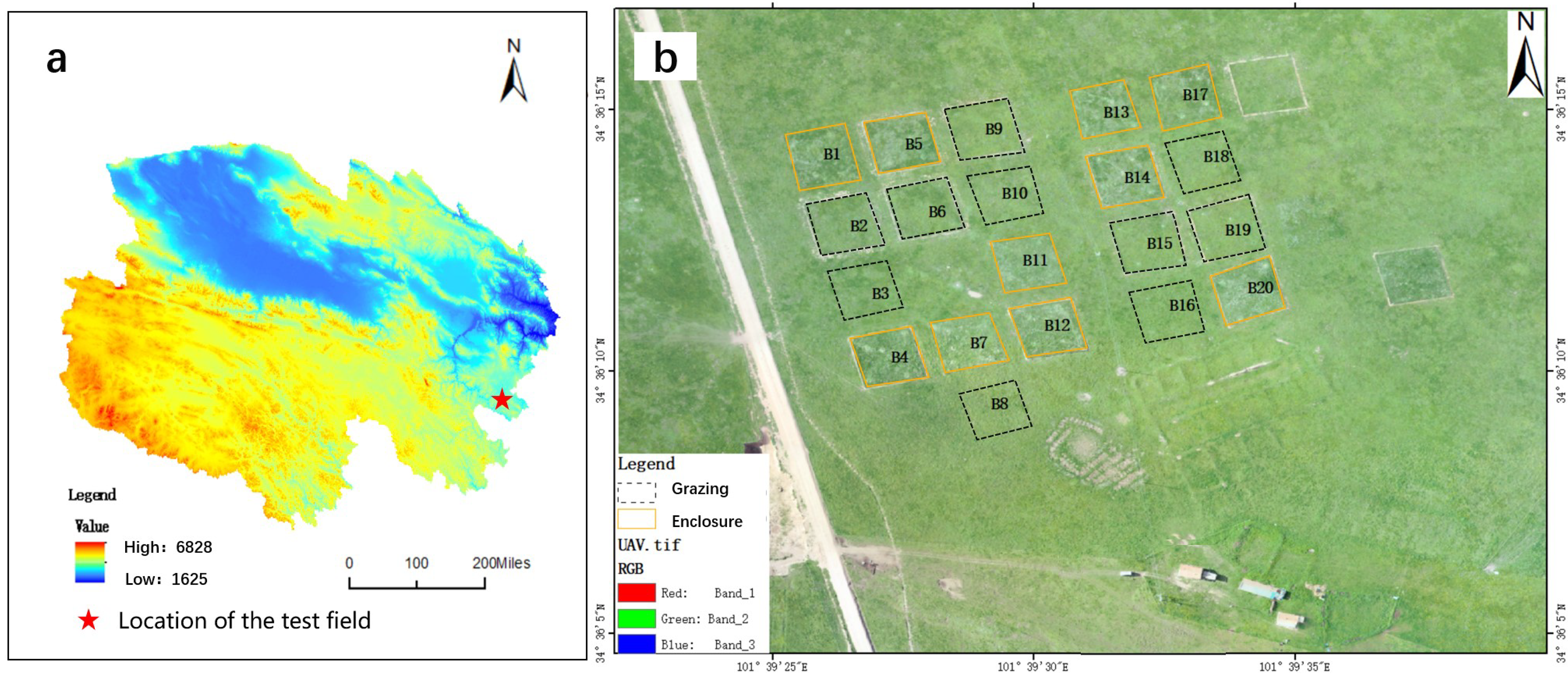
2.1. Study Area

At an average altitude of around 3400 m, the research region (Figure 1) is located at 34°36′N and 101°39′E in Henan County, Qinghai Province, on the eastern side of the Qinghai–Tibet Plateau. The climate is alpine and desert, with 606.3 mm average annual precipitation, mostly between May and September, and 1414.6 mm average annual evaporation. The average annual temperature is −1.3 to 1.6 °C, with a frost-free period of approximately 90 days; the average annual sunlight duration is 2564.5 h, and the total annual solar radiation is 146.2 MJ/m². Weeping grass, grass, early grass, gooseberry, ancient stork grass, and pearl bud polygonum are the predominant vegetation species in the test area, which corresponds to the alpine meadow type. We set up 20 sample plots, each with a 30 m × 30 m area, and low disturbance (i.e., slope less than 2°) within each plot. The blocks were spaced more than 10 m apart to allow passing and buffering. Ten of the sample plots were enclosed, while the other ten were allowed to be freely grazed.

2.2. Collection of Data

The spectrum data of the alpine grassland were gathered utilizing the dual-beam spectral simultaneous measuring equipment from Analytical Spectral Devices Inc. (ASD) due to the unpredictable and rapidly changing climate on the Tibetan plateau. The system comprises two ASD FieldSpec 4 feature spectrometers and a dual simultaneous measuring software system [49]. This technology allows reference whiteboard and target data to be acquired simultaneously under equal illumination conditions, considerably increasing their efficiency and allowing for optimal measurements in the field. The spectral range of the instrument is 350–2500 nm, with a wavelength precision of 0.5 nm and a spectral resolution of 3 nm@700 nm wavelength and 8 nm@1400/2100 nm wavelength [50].

The field survey was conducted from July to September in 2019 and 2020. In the test site, a total of 20 sample plots were constructed, as described above, each with 10 quadrats of 0.5 m × 0.5 m size and a cover requirement of above 85%. A total of 400 sample squares were gathered in early July, 400 sample squares in mid–late August, and 400 sample squares in mid-September, for a total of 1200 sample squares collected across two years; each sample was repeated six times for a total of 7200 spectral data points. For each quadrat, the cover, dominant species, longitude, latitude, and whether or not it was grazed was recorded, and the average observed plant height was used to calculate the average grass height for the entire quadrat. The herbaceous plants were mowed flush after spectral data collection, and the fresh biomass was weighed immediately using an electronic scale.

2.3. Methods and Flow of Data Processing

2.3.1. Pre-Processing of Data

After exporting the spectrum data with ViewSpec Pro, MATLAB was used to conduct Savitzky–Golay (SG) smoothing and denoising [51]. The SG filter created a generally smooth spectral curve while also retaining the absorption properties at all wavelengths. The spectra were determined after the spectral curves with major discrepancies and errors were deleted, yielding a total of 7200 spectra. The six spectra of each sample were averaged into a composite spectrum, yielding a total of 1200 valid hyperspectral data points.

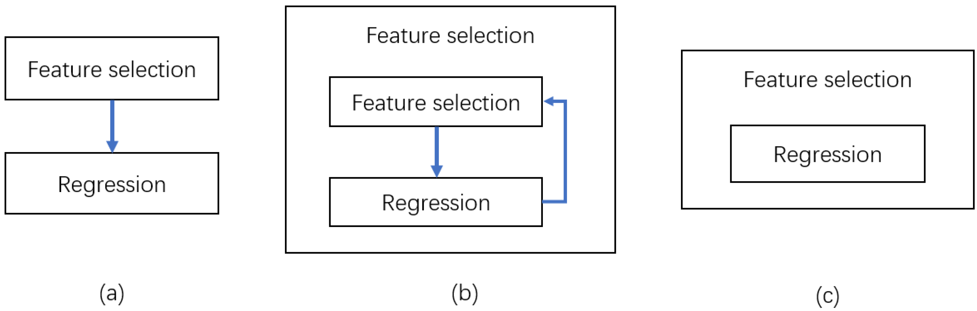
2.3.2. Feature Selection

Because full-band hyperspectral data contain a large amount of redundant information and their dimensionality is usually high, the direct modeling of these data will likely cause problems such as poor computational efficiency and overfitting; thus, feature selection is required to lower the spectral dimensions of the data. Feature selection is the process of picking the most important attributes from a large number of options to create a more effective model [52,53]. The original spectral feature characteristics are unchanged; rather, an optimal subset of them is selected. Feature selection and machine learning algorithms are tightly linked, and feature selection strategies can be classed as filter, wrapper, or embedded based on a combination of the subset assessment criteria and subsequent learning algorithms [40,54].

• Filter feature selection

The filter model, as shown in Figure 2, uses feature selection as one of its preprocessing steps, with the evaluation of the selected feature subset based primarily on the characteristics of the data set itself [55]. As a result, the filter model is independent of the learning algorithm and directly evaluates the features, ranks them according to their importance, and then removes the features with low scores. We select the following three filtering feature selection algorithms.

The Chi-square test (CHI), a filtering method, is used to capture the linear relationship between each feature and the label [56]. By calculating the Chi-square statistic between each non-negative feature and the label, the features are ranked from highest to lowest according to the Chi-square statistic. The Chi-square statistic is a measure of the difference between the distribution of the index data and the chosen expected or assumed distribution. It was proposed by the British statistician Pearson in 1900. It is obtained by dividing the square of the difference between the actual observation times ($f_0$) and the theoretical distribution times ($f_e$) by the theoretical times and then summating them. Its calculation formula is as follows:

$$x^2={{\displaystyle \sum \frac{\left(f_0-f_e\right)}{f_e}}}^2$$

(1)

Linear regression (LR) determines which independent variables are correlated with dependent variables [57]. Linear regression is a common model in machine learning tasks. It is actually a broad concept and usually refers to a set of independent variables to predict the dependent variable. The formula is as follows:

$$y={\beta }_0+{\beta }_1{x}_1+\cdots +{\beta }_n{x}_n+\epsilon$$

(2)

where ${\beta }_n$ is the coefficient of the regression model, $y_i$ is the observation vector of the dependent variable, $x_n$ is the observation value of the independent variables, and $\epsilon$ is a random error.

In addition, the linear regression model can also answer another question: that is, among all the normalized independent variables, which variables are the most important and which are not important. If features are essentially independent of each other, even the simplest linear regression models can achieve excellent results on low-noise data or data that significantly outnumber the number of features of interest. The least square method can be used to calculate the $\stackrel{⌢}{\beta }$ order, according to the order analysis of its importance.

$$\stackrel{⌢}{\beta }={({\beta }_0,\cdots ,{\beta }_n)}^T={(X^{T}Y)}^{-1}{X}^{T}Y$$

(3)

where $\stackrel{⌢}{\beta }$ is an estimate of the coefficient, ${\beta }_n$ is the coefficient of the regression model, $y_i$ is the observation vector of the dependent variable, $X$ is the independent variable matrix, $X^T$ is the transpose of $X$, and $Y$ is the dependent variable matrix.

The maximum information coefficient (MIC) is used to mine linear and nonlinear relations between continuous variables through discretization optimization with unequal intervals [58], and the non-functional dependence between features can also be extensively mined. The calculation method of the maximum information coefficient is as follows.

Mutual information and meshing methods are used for the calculation. Mutual information can be regarded as the amount of information contained in a random variable about another random variable, or the uncertainty reduced by a random variable due to the fact that another random variable is known. In this experiment, the mutual information $I\left(F;R\right)$ of aboveground biomass $\left(F\right)$ and spectral variables $\left(R\right)$ is defined as

$$I\left(F;R\right)={\displaystyle \sum {\displaystyle \sum p(F,R){\log }_2\frac{p(F,R)}{p(F)p(R)}}}$$

(4)

where $p(F,R)$ is the joint probability density of $F$ and $R$, and $p(F)$ and $p(R)$ are the marginal probability distribution densities of $F$ and $R$ respectively.

Consider $F$ separately with each $R$ as a data set; the value range of $F$ is divided into a intervals, and the value range of $R$ is divided into b intervals, so on the scatter plot of $F-R$, all the points are divided into range a * b. Data sets in different interval division methods will obtain different data distributions, and the maximum value in different interval division methods is the maximum information value. The maximum information coefficient ($MIC$) is obtained after normalization, and its mathematical expression is

$$MIC\left(F;R\right)={\max }_{(a\times b)<B(n)}\frac{I(F;R)}{{\log }_2\min (a,b)},B(n)=n^{0.6}$$

(5)

where $n$ is the data size.

The maximum information coefficient is a standard to measure the correlation between two variables (including linear correlation and nonlinear correlation). According to the formula, its value is distributed between 0 and 1. The larger the value is, the stronger the correlation is; otherwise, the weaker it is.

• Wrapped feature selection

Wrapped feature attribute selection is often based on a specific learning algorithm, such as regression; the performance of the feature attribute subset in that learning algorithm is determined by whether this subset meets the data sample selection requirements [59]. The worth of the feature subsets is determined directly by the regression, and the feature subsets that perform well in the training and learning process are selected first in this model. Figure 2 depicts the technique selection process.

The basic principle behind recursive feature elimination (RFE) is to iteratively create a model (for example, a support vector machine (SVM) or linear regression (LR) model), select the best features, and then repeat the process for the rest of the features until all the features have been explored [60]. In this process, features are arranged in the order in which they are deleted. Therefore, this is a greedy method to determine the best collection. Below, we use the classical SVM-based RFE algorithm (RFE_SVM) to discuss this algorithm.

Firstly, k features are input into the SVM regression as the initial feature subset, the importance of each feature is calculated, and the prediction accuracy of the initial feature subset is obtained by the cross validation method. Then, the feature with the lowest importance is removed from the current feature subset to obtain a new feature subset, which is input into the SVM regressor again to calculate the importance of each feature in the new feature subset, and the prediction accuracy of the new feature subset is obtained by using the cross-validation method. Finally, the recursion repeated until the feature subset is empty. Finally, k feature subsets with different number of features are obtained, and the feature subset with the highest prediction accuracy is selected as the optimal feature combination [61]. The RFE algorithm based on the linear regression model (RFE_LR) involves a similar calculation process.

• Embedded feature selection

Embedded feature selection mixes feature attribute selection with a learning algorithm that searches for the best set of feature attributes while constructing a data model [62]. Under the condition of a given regression, this method type blends the feature attribute space with the data model space and embeds the selection of feature attributes into the regression, while the corresponding learning algorithm still evaluates the feature attribute set. The embedded algorithm procedure is challenging; however, it has the advantages of filtered feature attribute selection and encapsulated feature attribute selection, which help to achieve both efficiency and accuracy.

Lasso regression is a new variable selection technique proposed by Robert Tibshirani in 1996 [63]. Lasso is a contraction estimation method. Its basic idea is to minimize the sum of squares of residuals under the constraint that the sum of absolute values of regression coefficients is less than a constant, so that some regression coefficients strictly equal to 0 can be generated, and further explicable models can be obtained. In the case of processing a large number of variables or with sparse variable matrix processing, this shows obvious advantages. Lasso achieves compression estimation by constructing penalty functions to make the coefficient values of some variables equal to zero, which can not only simplify the model but also avoid overfitting [64]. The objective function of Lasso’s least square form is as follows.

Ridge modifies the loss function by adding the L2 norm of the coefficient vector. Ridge regression is a biased estimation regression method for collinear data analysis [65].The role of the Ridge is to improve the performance of the model by keeping all variables; for example, using all variables to build a model, while giving them importance. Because the Ridge keeps all variables intact, Lasso does a better job of assigning importance to variables [66]. The coefficients of the Lasso (Ridge) regression equation were normalized to 0–1 to obtain the feature score.

$$lasso:\underset{{\beta }_{0,}\beta }{\min }\{{\displaystyle \sum _{i=1}^N(y_i-{\beta }_0-{\displaystyle \sum _{j=1}^P{\beta }_j{x}_{ij}})+\lambda {\displaystyle \sum _{j=1}^P\left|{\beta }_j\right|}}\}$$

(6)

$$ridge:\underset{{\beta }_{0,}\beta }{\min }\{{\displaystyle \sum _{i=1}^N(y_i-{\beta }_0-{\displaystyle \sum _{j=1}^P{\beta }_j{x}_{ij}})+\lambda {\displaystyle \sum _{j=1}^P{\beta }_j{}^2}}\}$$

(7)

where ${\beta }_0,\beta$ is the coefficient of the regression model, $y_i$ is the observation vector of the dependent variable, $x_{ij}$ is the observation matrix of the independent variables, $N$ is the number of observed values and $P$ is the number of features, and $\lambda \ge 0$ is an adjustable parameter whose size is related to the sparsity of $\beta$. Lasso filters variables by adjusting the size of $\lambda$.

The random forest (RF) algorithm was first proposed by Breiman L.and is a machine learning algorithm based on classification and regression decision tree (CART) [67]. It can analyze the importance of thousands of input features. The main idea is to integrate the results of multiple decision trees to conduct an overall analysis of classification tasks, and the specific implementation process is as follows:

(1)

Construct the training sample set: parts of the samples are randomly selected from the original sample set to form the training sample set (Bootstrap method). N training sample sets could be obtained after repeating N times.

(2)

Establish N CART decision trees: Based on the samples in the training sample set, firstly M features are randomly selected from all input features M (node random splitting method), and then M features are constructed according to the variance impurity index. The calculation formula is as follows:

$$i(N)={\displaystyle \sum _{i\ne j}P(w_i)P(w_j)}=1-{\displaystyle \sum _j^{}{P}^2(w_j)}$$

(8)

where $w_i$ is a attribute of class $i$, $w_j$ is the frequency of $w_j$ samples in the total samples at node N, and $i$ is variance impurity.

Set a threshold for the decrease of variance impurity. If the decrease of variance impurity behind the branch is less than this threshold, the branch is stopped. At this point, the construction of N decision trees is completed.

(3)

Overall planning of decision tree results. All the constructed decision trees are formed into a random forest, the random forest regressor is used to predict, and finally the result is determined by voting.

Random forest can rank the importance of input features. During Bootstrap sampling, about one-third of the original data is not extracted, which is called out-of-bag data (OOB). The OOB error generated by OOB data can be used to calculate the importance of each input feature, from which feature selection can be carried out [68]. The expression of feature importance assessment model is

$$FE(M_A)={\displaystyle \sum _{t=1}^N(E_{n_t}^{M_A}-E_{O_t}^{M_A})/N}$$

(9)

where $FE$ is the characteristic importance, $M$ is the total number of features, $N$ is the total number of decision trees, $E_{O_t}^{M_A}$ is the OOB error value of the t-th decision tree before adding noise to feature $M_A$, and $E_{n_t}^{M_A}$ is the OOB error value of the t-th decision tree after adding noise to feature $M_A$. If the OOB error increases significantly and the accuracy loss is large after adding noise to feature $M_A$, it indicates that the input feature is of high importance.

2.3.3. Methods of Model Construction

To evaluate and analyze the effectiveness of several feature selection algorithms for simulating natural alpine meadows, AGB prediction models were built using support (SVM), Gaussian process regression (GPR), least squares regression boosting (LSB), and artificial neural network (ANN) approaches.

SVM is an exceptionally strong and adaptable supervised learning technique for classification and regression [69]. SVM’s purpose is to use dividers (lines or curves in 2D space) or streamers (curves, surfaces, etc. in multidimensional space) to create a classification hyperplane that not only accurately classifies each sample but also separates them [70]. Support vector machines are essentially boundary maximization evaluations since the resultant classification hyperplane not only correctly classifies each sample but also makes the closest sample of each class as far away as possible from the classification line (i.e., the hyperplane).

Gaussian process regression (GPR) is a nonparametric regression model that uses a Gaussian process (GP) prior to data analysis [71,72]. The GPR model assumptions include both noise (regression residuals) and a Gaussian process prior, which is solved using Bayesian inference [73]. In addition, GPR can provide a posteriori information of the predicted results, and the posteriori information has an analytic form when the likelihood is in a normal distribution. As a result, GPR is a generalizable and resolvable probabilistic model [74].

Predictive models built from weighted combinations of multiple individual regression trees are known as regression tree ensembles. Boosting algorithm is an ensemble learning algorithm that can transform a weak learner into a strong one. Least squares regression boosting (LSB) is one of the boosting methods using least squares as the loss criterion [75]. The integration trees constructed by LSB select only one feature in each round to approximate the alignment accuracy residuals and fit the regression set well by minimizing the mean.

Artificial neural networks (ANNs) are information processing systems based on emulating the structure and operations of neural networks in the brain, simulating neuronal processes with mathematical models [76,77]. The features of ANN include self-learning, self-organizing, self-adaptation, and strong nonlinear function approximation capabilities, as well as fault tolerance.

The machine learning algorithms were tested using a five-fold cross-validation method. In this approach, the data set was separated into five parts, with four serving as training data and one serving as test data for the test.

The coefficient of determination (R²) and root mean square error (RMSE) were used as accuracy evaluation methods. Higher R² values suggest more accurate modeling. The RMSE measures the model’s predictive capacity, and its magnitude is inversely proportional to the model’s accuracy.

ASD ViewSpec Pro, SPSS 26, Matlab 2020, and Spyder (Python) software were used for data handling [78].

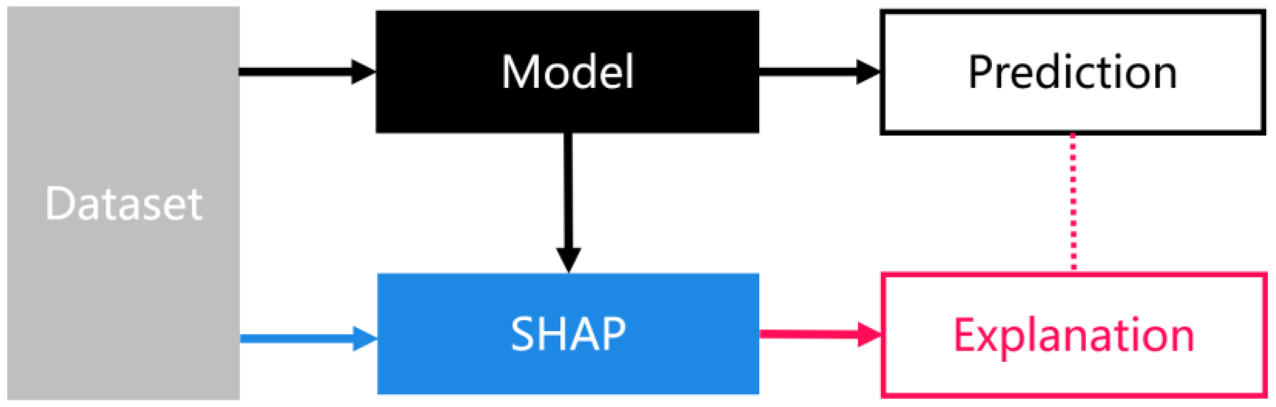
2.3.4. Interpretability Based on SHAP Values

The Shapley value was first proposed by Lloyd Shapley—a professor at University of California, Los Angeles [79]. Its initial research objective was to help solve the problems of social contribution and the distribution of economic benefits in the process of economic cooperation or a game. For example, if there are N people cooperating, due to their different abilities, each member’s contribution will be different, and the distribution of benefits will be different. The optimal distribution is as follows: individual contribution is equal to individual benefit. The Shapley method quantifies the contribution rate and profit distribution. The Shapley value refers to the amount of money those individual members earn on a project equal to their own contribution level. The Shapley Additive Explanations (SHAP) package is a model interpretation package developed in Python that can be used to interpret the output of any machine learning model [80]. The model interpretation method based on the Shapley value is a post-model interpretation method independent of the model. As shown in Figure 3, the process of model prediction and SHAP interpretation are two parallel processes, and SHAP interprets the results of model prediction. Its main principle is as follows: the SHAP value of a variable is the average marginal contribution of this variable to all special sequences. SHAP constructs an additive explanatory model inspired by cooperative game theory, in which all variables are regarded as “contributors”.

The main advantage of the SHAP value is that it can reflect the influence of independent variables in each sample, and it can also show the positive and negative factors of its influence [81]. A significant advantage of some machine learning models is that they can consider the importance of the independent variable of the model results; the variable importance has a variety of traditional calculation methods, but the traditional calculation method of variable importance effect is not good, and the traditional variable importance can only tell which variables are important, but not shed light on how the variable affects the forecasting result. The SHAP method provides another way to calculate the importance of variables: take the average of the absolute value of the SHAP value of each variable as the importance of the variable and obtain a standard bar chart, which can simply and clearly show the ranking of the importance of the variable. Further, to understand how a single variable affects the output of the model, we can compare the SHAP value of the variable with the variable values of all the samples in the dataset. The SHAP package also provides extremely powerful data visualization capabilities to show the interpretation of a model or prediction.

The complete data analysis process is showed in Figure 4.

3. Results

3.1. Data Exploration and Analysis

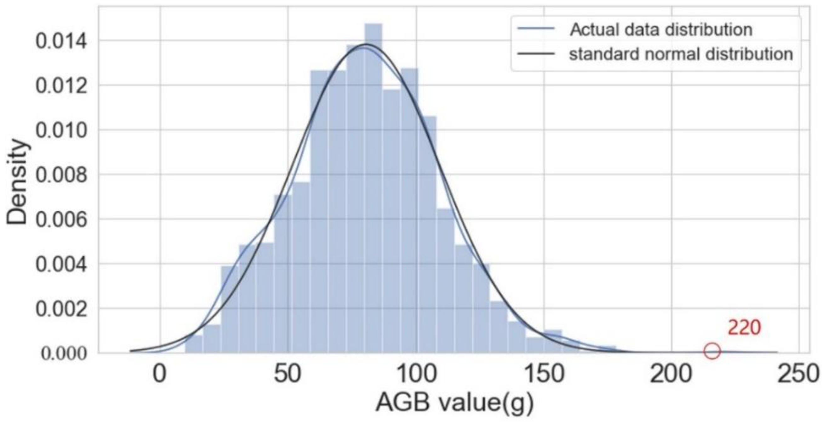
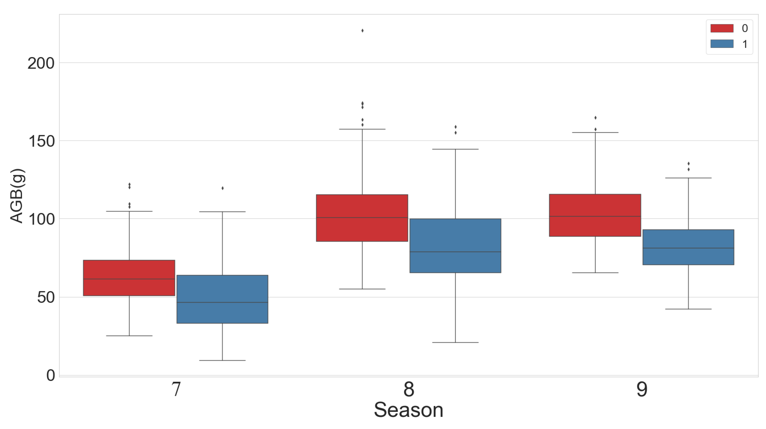
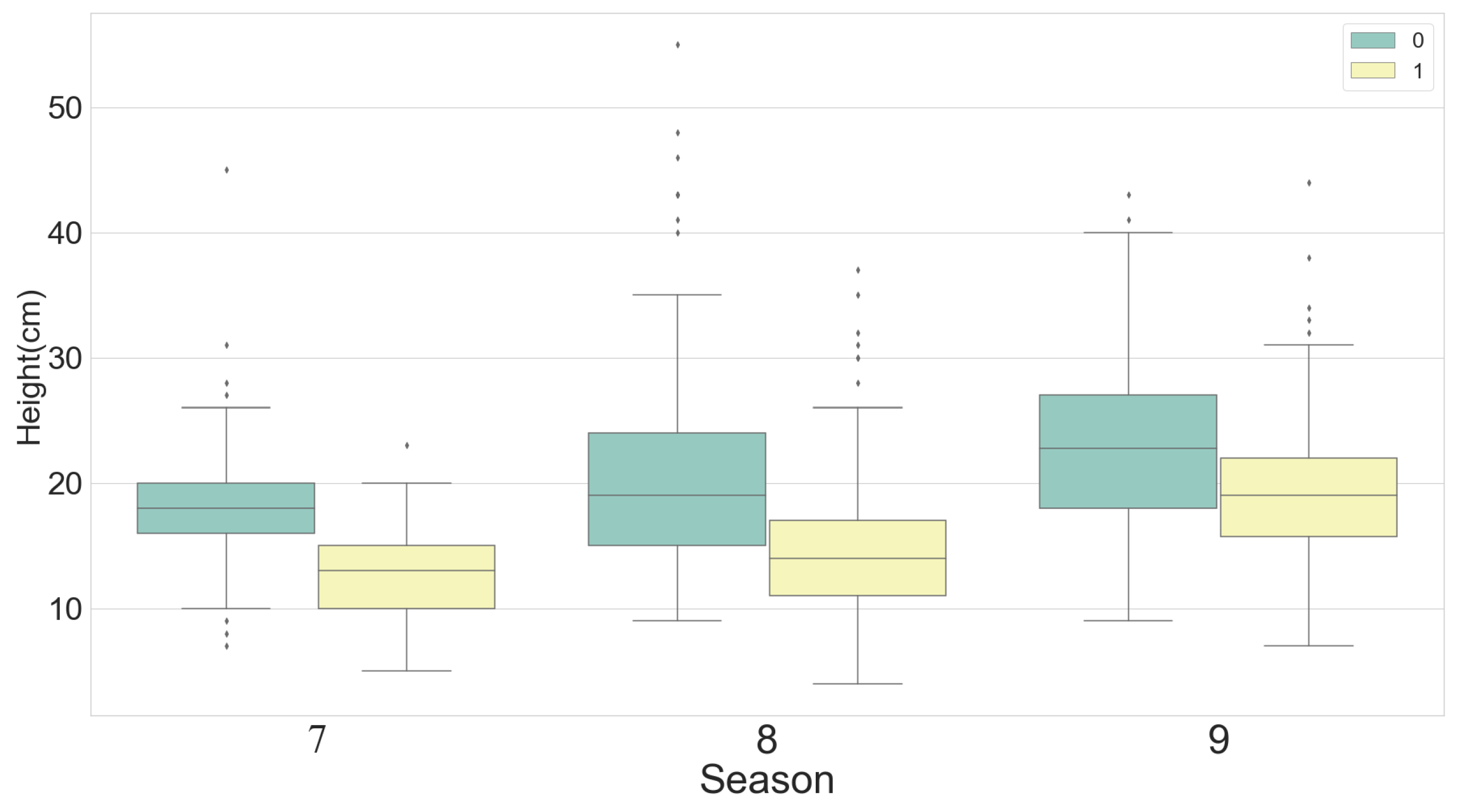
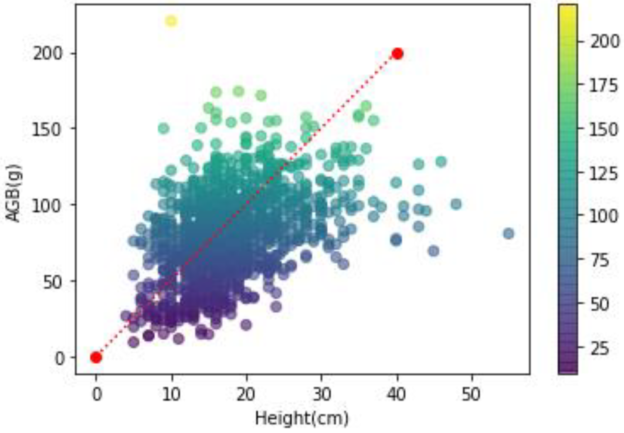
3.1.1. Statistical Analysis of Ecological Data

The AGB of all 1200 samples was used to create a histogram (Figure 5); the data were found to be almost normally distributed, indicating that there were sufficient data points used in the experiment. The AGB of one sample was anomalously large (220 g), which made the right tail of the histogram longer; however, the difference was not significant. These findings are consistent with the expected behavior of natural grassland—that is, the biomass is concentrated in a range, and the proportion of large values is very small.

The mean AGB value was 80.5779 g, with a coefficient of variation of 0.358 based on a descriptive statistical analysis of the ground survey data (

Table 1. Statistical analysis of AGB and grass height data.

Parameter	Unit	N	Min	Max	Mean	SD	CV
AGB	gram	1200	9.35	220.54	80.5779	28.884	0.358
Height	centimeter	1200	4	55	18.578	6.702	0.372

), indicating a large variation. The mean grass height was 18.578 cm, with a coefficient of variation of 0.372, also indicating significant fluctuation.

3.1.2. Correlation Analysis of Ecological Data

To ensure a balanced data population, the same numbers of samples were grazed and not grazed, with the same number of samples taken for each growing season. Box graphs were constructed showing samples from different categories (Figure 6). Average AGB and grass height both showed an increasing trend over time; however, the AGB increase between July and August was greater than that recorded from August to September. The maximum grass height and AGB values were both recorded in August. The AGB and grass height values in the not grazed area were higher than those in the grazed area.

The analysis of variance (ANOVA) studies the contribution of variation from different sources to total variation to determine the influence of controllable factors on research results. A two-way ANOVA performed on AGB showed significance values of 0.000 (i.e., less than 0.01) for both growing season and grazing situation variables. The value for the interaction between the growing season and grazing situation was 0.012 (i.e., greater than 0.01). As a result, it can be inferred that both the growing season and the grazing scenario had a substantial impact on AGB, with the interaction between the two having a greater impact (p-value of 0.05).

Similarly, a two-factor ANOVA was conducted on grass height; the results indicate that growing season, grazing condition, and the interaction between the two all had a significant effect on grass height.

Drawing scatter plots of AGB and grass height (Figure 7), it can be seen from the figure that the overall distribution of scattered points is clumped, and there are some isolated points. This indicated that there was no obvious linear relationship between AGB and grass height. By quantitative correlation analysis, there was a linear relationship between AGB and grass height (significance of 0.000) with a correlation coefficient of 0.424.

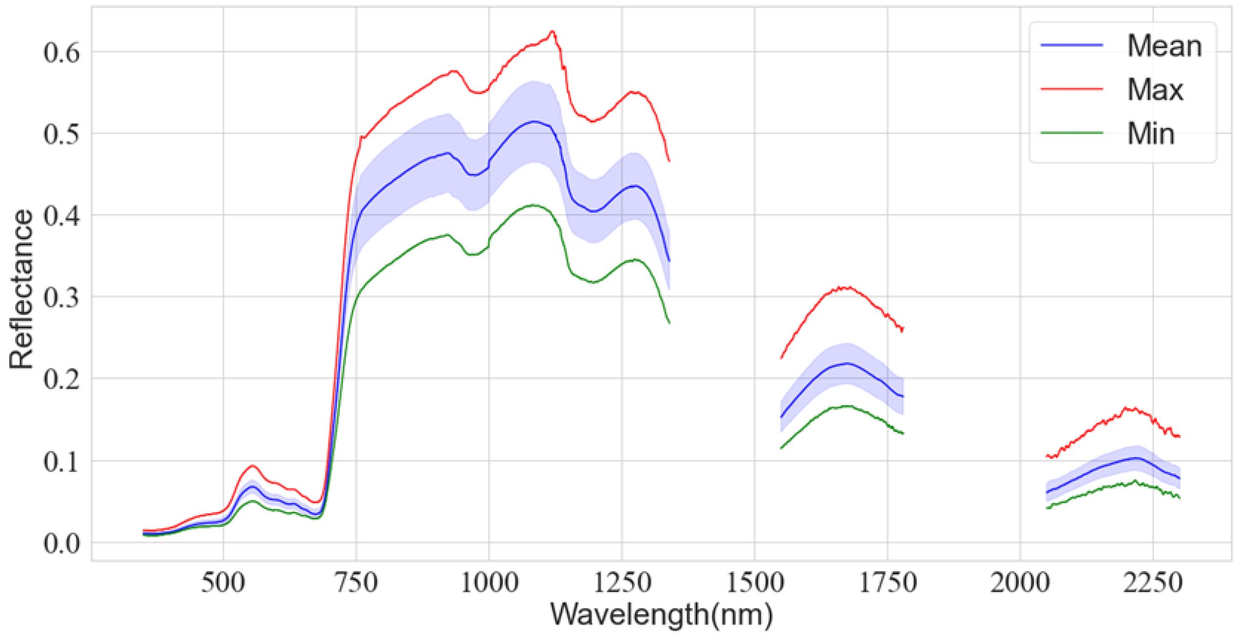
3.1.3. Spectral Data Analysis

The spectra were all plotted on a single graph (Figure 8). The grassland’s spectral structure is typical of vegetation, with visible absorption valleys and reflection peaks. Because the range ~2300 to 2500 nm is near the edge of the spectrometer band, and the reflectance ranges of ~1340 to 1550 nm and ~1780 to 2050 nm are affected by the water absorption of the leaves, the noise in these bands is high; this affects the modeling, and thus these parts of the data were removed and the remaining bands were used for analysis.

3.2. Feature Selection

Each spectral parameter is given a score by the feature selection algorithm: the greater the score, the more important the parameter is. The top-ranking feature parameters are then chosen as the final parameters. The feature selection analysis was carried out on both the pure spectral and multi-source data.

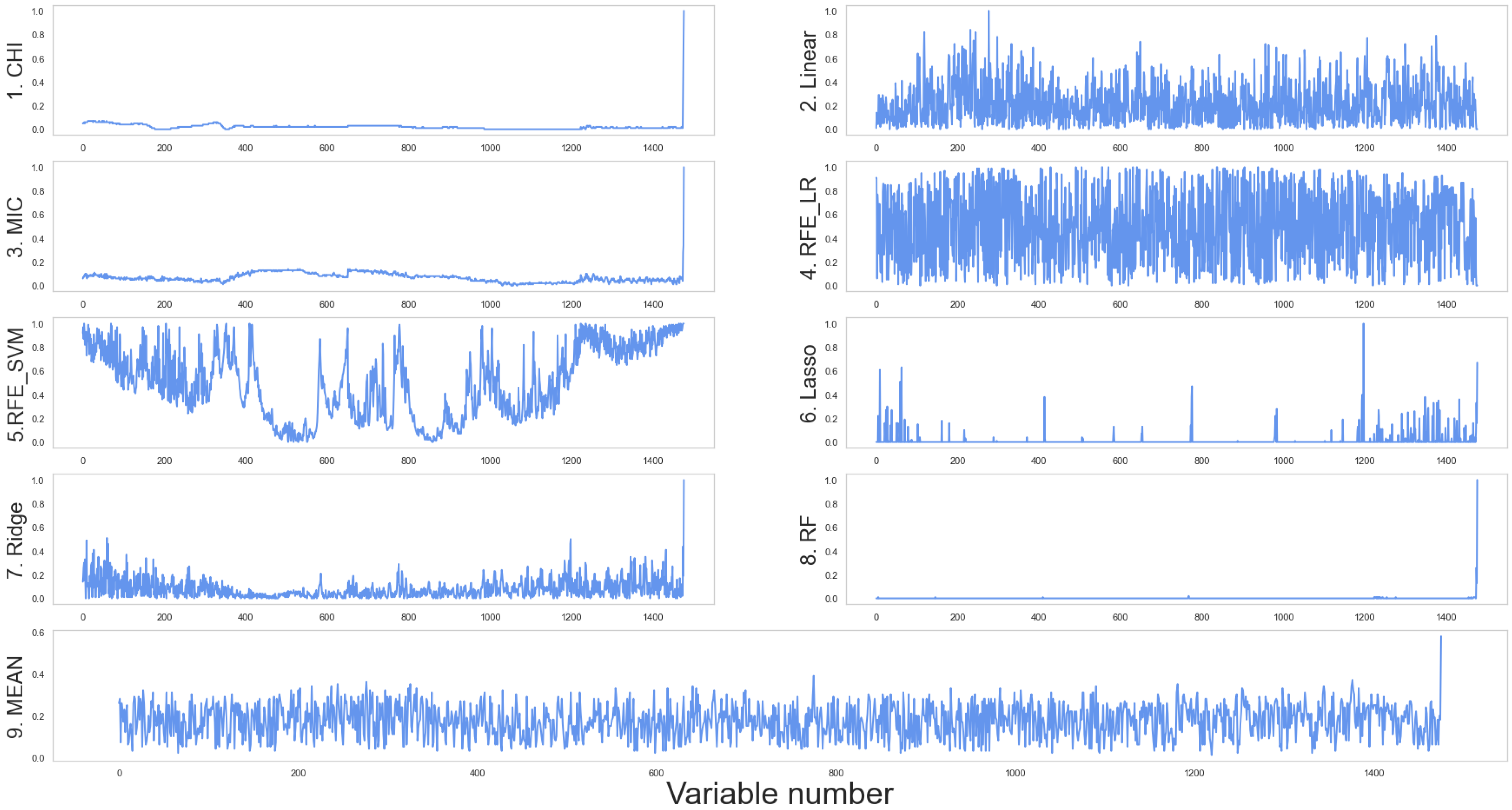
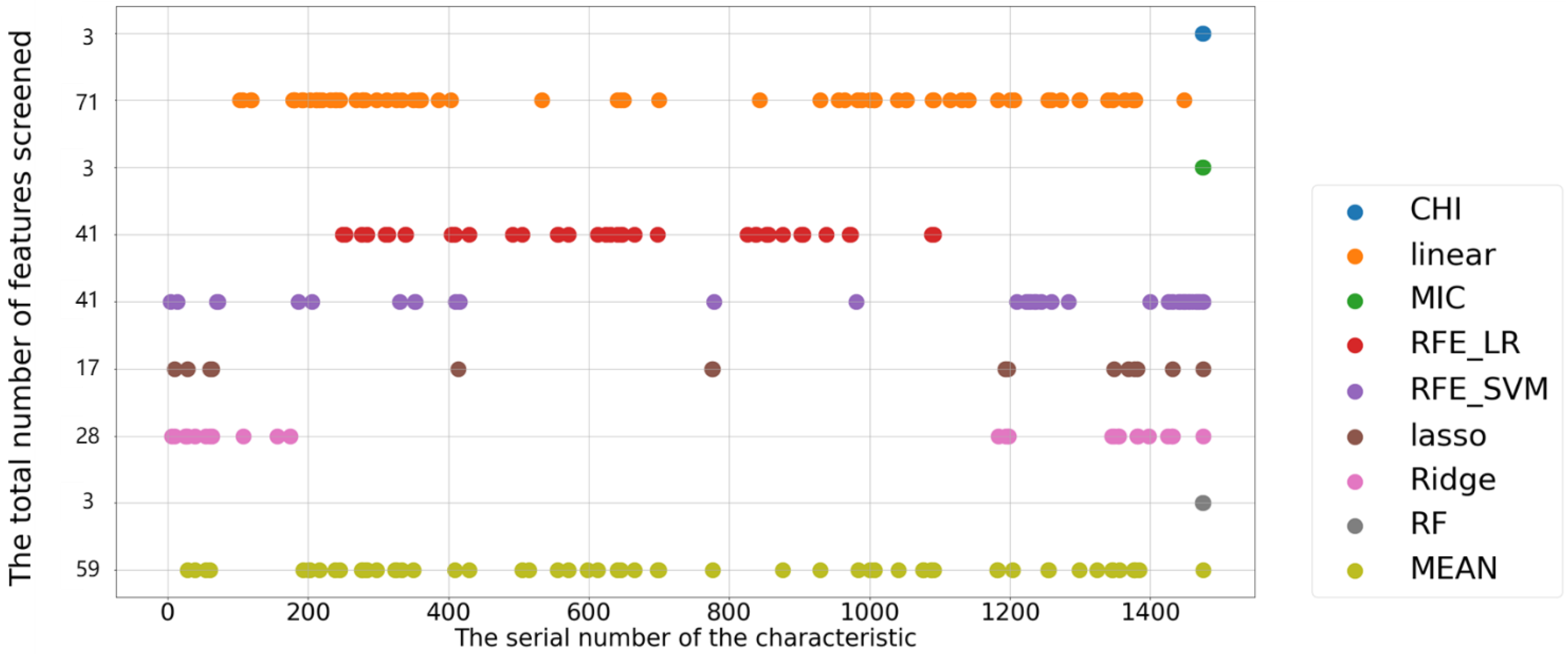
3.2.1. Spectral Data-Based Feature Selection

• Scoring of features based on pure spectral data

The spectral data were processed using several feature selection methods to determine the score of each band (minimum 0 and maximum 1), the results of which are displayed in Figure 9. The details of the individual curves are as follows. (1) The overall Cor curve is reasonably smooth; the neighboring band scores are close to each other without discarding redundancy between variables, allowing the band intervals to be identified with high correlation. (2) The linear scoring may quantify the linear relationship between spectra and AGB; however, it also singles out the correlation characteristics of all relevant features—i.e., numerous higher score values emerge surrounding each individual high score. For example, high scores near variable 200 are densely distributed, and the wide bar chart contains several adjacent bands. (3) The MIC and CHI curves are generally similar, showing linear relationships between the independent and response variables as well as nonlinear ones. The MIC curve, however, does locally show a major excursion compared to Cor. (4) The RFE_LR curve is based on linear regression model optimization, which is more prone to bipolar evaluation overall; however, the distribution of high and low scores is relatively uniform, and the feature selection performance is poor. (5) The RFE_SVM scores show considerable unpredictability and volatility, with visible valleys and a broad distribution of peaks. (6) The Lasso approach can successfully select a limited number of critical feature variables while allowing the scores of the majority of other features to converge to zero. It is particularly useful when the number of features needs to be reduced; however, it is not very effective when trying to interpret data. (7) The Ridge approach scores each linked variable equally, as shown in Figure 9, and the scores of close bands are extremely similar. (8) After assigning a few characteristics with the highest ratings, the RF approach scores the other factors considerably lower. (9) Overall, when all of the features are averaged, most of the variables have values between 0.1 and 0.5.

2.

Selection of features based on pure spectral data

Variable selection is performed for spectral data according to the score, with the results displayed in Figure 10. The bands selected by Cor are clustered in the leftmost region of the plot because the algorithm scores this section of the spectrum the highest and ranks it first, thus resulting in this method not selecting other crucial parts of the spectrum with a high degree of multicollinearity. The linear approach’s chosen bands are notably dispersed. To choose features, the MIC approach focuses on various nearby bands; thus, the results of this selection method are clustered. The RFE_LR approach’s bands cover a wide range of frequencies, some of which are close to those of the linear approach. The RFE_SVM and Lasso selections produce comparable results, with dense band selection in certain regions and sparse selection in others. The Ridge findings are similar to those of Lasso, but they span fewer regions and have more continuous bands. The RF results are similar to those of the Lasso selection method but are less dispersed.

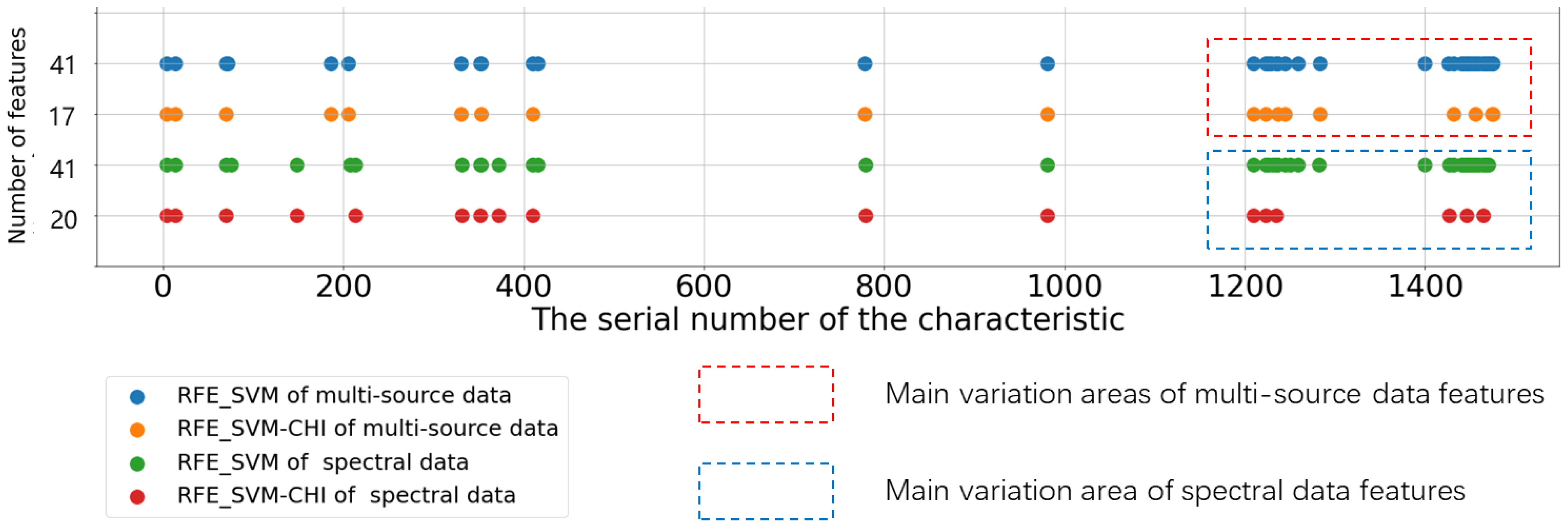
3.2.2. Multi-Source Data-Based Variable Score Analysis

The feature selection analysis was re-run after adding grass height, season, and grazing condition (i.e., grazing or non-grazing) to the pure spectral data to compose multi-source data. Given the differences in data sources, the different methods showed substantial variability in their evaluation of the three newly added factors (

Table 2. Scores of three factors in different feature selection.

Factor	CHI	Linear	MIC	RFE_LR	RFE_SVM	Lasso	Ridge	RF	Mean
Grazing conditions	0.32	0	0.28	0	1	0.33	0.44	0.26	0.2
Height	0.59	0	0.34	0	1	0.16	0.19	0.16	0.18
Season	1	0	1	0	1	0.67	1	0.67	0.58

). Both linear and RFE_LR approaches identify these features as worthless, whereas RFE_SVM identifies them as the most important. Based on the mean values of all methods, the season is the most important factor, which is consistent with the ecological experience of grass. This also demonstrates that the spectrum provides a more accurate representation of grass height and grazing. A temporal term such as season, however, cannot be directly represented by the spectrum without a priori understanding.

(1)

Multi-source data-based feature scoring

In terms of variable selection, the CHI, MIC, and RF algorithms show the most significant differences in terms of results when compared to the pure spectral data analysis model (Figure 11). All three algorithms treat the three newly added elements as important variables and effectively ignore the effect of the spectrum; the RF algorithm is easy to overfit, the search converges too quickly, and the results are not ideal. The RFE_LR, RFE_SVM, and linear models are the most stable; in these approaches, the band’s fractional value changes only slightly. With some image form alterations, the Lasso and Ridge approaches are stable. The Lasso approach produces sparse models, which are beneficial for selecting feature subsets; however, Ridge performs more consistently than Lasso since the valuable features tend to correlate to non-zero coefficients. As a result, the Ridge approach was deemed suitable for data comprehension.

(2)

Feature screening based on pure multi-source data

The results of variable screening utilizing nine different types of multi-source data are depicted in Figure 12. The image reveals that only three important variables, i.e., CHI, MIC, and RF, are chosen, indicating that these three variables really do matter and their relatively faster convergence, which does not take spectral effects into account, compared to other algorithms. Because the algorithm itself evaluates the relationship between the independent and dependent variables when evaluating their importance and does not consider interaction relationships, the results of the linear and RFE_LR approaches do not differ substantially; RFE_IR is an optimized upgrade of the linear approach with similar results. RFE_SVM is essentially the original variable multiplied by three significant variables. In contrast, the Lasso method introduces three factors while drastically reducing the number of other spectral variables. The Ridge approach, like Lasso, was also able to decrease the number of variables.

In conclusion, among the nine feature selection algorithms, the Lasso algorithm performs well. Firstly, it does not ignore the spectral information due to data changes such as CHI, MIC, and RF (only three variables are selected). Secondly, compared with linear and RFE_LR approaches, in which a large number of highly correlated (adjacent) variables were selected, Lasso was able to suppress feature multicollinearity well (such as in Figure 11, Lasso’s score for most of the variables was always biased to 0). Finally, the characteristics for which it screens, which are few in number but widely distributed, avoid the risk of over-selection. The variable screening results of RFE_SVM and Ridge are similar to those of Lasso, but both have the situation of screening adjacent spectra. Therefore, we improve RFE_SVM, perform CHI calculation on the screened features of RFE_SVM, remove the redundant features with high linear correlation, and finally simplify the features. The results are shown in Figure 13. The number of features is significantly reduced in the two different data sets, and the main variation area is between variables 1200 and 1500. Combined with the feature selection part of RFE_SVM mentioned above, we know that the feature score of this area is mostly high and fluctuates greatly.

3.3. Model Construction and Evaluation

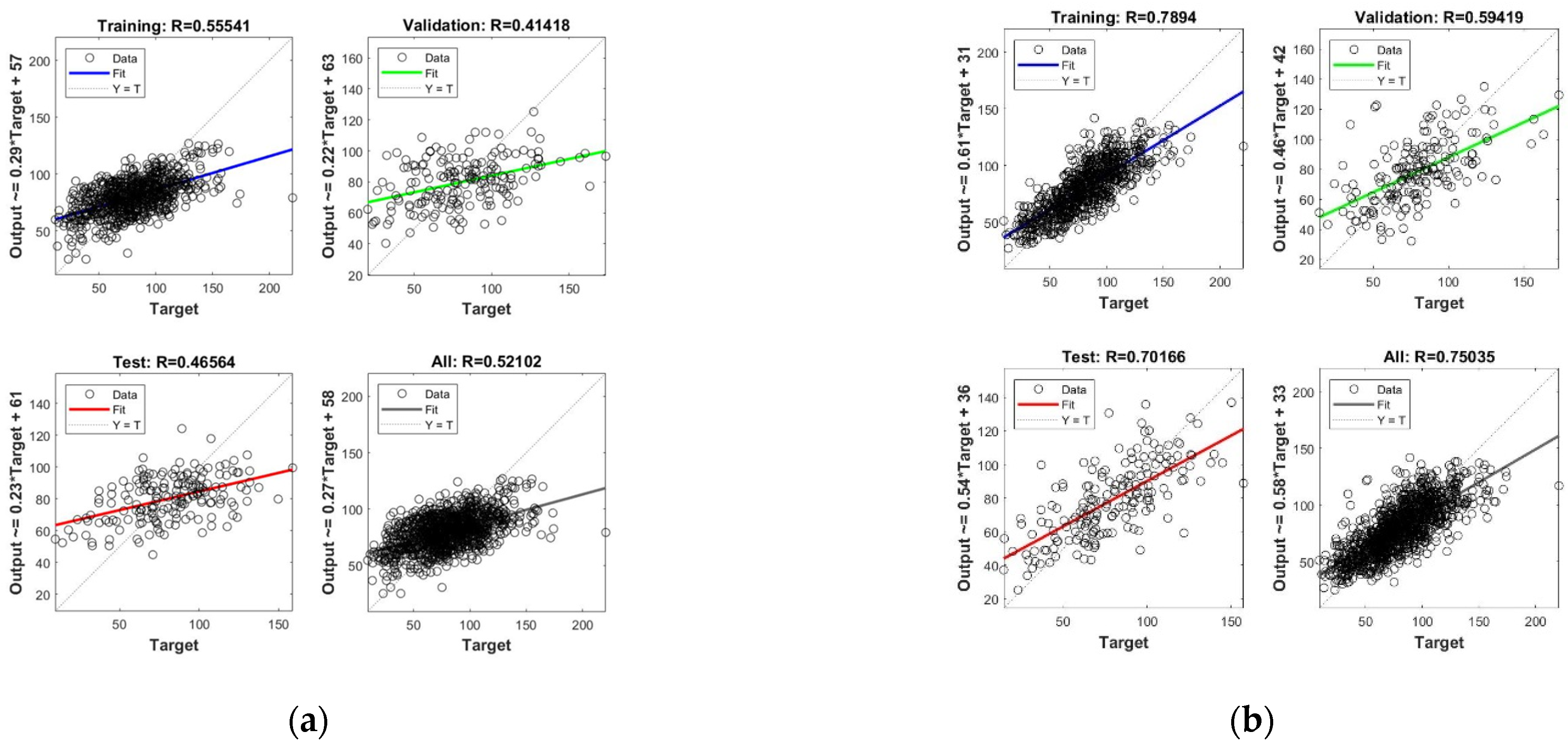
3.3.1. AGB Inversion Model Based on Machine Learning

Pure spectral data and multi-source spectral data after feature selection were used as independent variables in the AGB prediction models. SVM, GPR, and integrated tree regression models (LSB) were built with the observed AGB as the response variable.

Table 3. Regression results based on different feature selection models.

Feature Selection		Evaluation Index	Dataset
			Spectral Data			Multi-Source Data
			SVM	GPR	LSB	SVM	GPR	LSB
Filter	CHI	R2	0.04	0.02	−0.06	0.38	0.48	0.46
		RMSE	28.267	28.615	29.744	22.748	20.909	21.323
	Linear	R2	0.07	0.07	−0.05	0.09	0.08	−0.03
		RMSE	27.798	27.887	29.542	27.554	27.707	29.337
	MIC	R2	0.02	0.04	−0.05	0.38	0.48	0.47
		RMSE	28.554	28.554	29.552	22.75	20.811	21.058
Wrapper	RFE_LR	R2	0.07	0.05	−0.03	0.08	0.06	−0.03
		RMSE	27.799	28.206	29.552	22.750	20.811	21.058
	RFE_SVM	R2	0.09	0.10	−0.01	0.38	0.47	0.48
		RMSE	27.536	27.416	29.07	22.667	20.96	20.832
	RFE_SVM-CHI	R2	0.06	0.08	0	0.38	0.53	0.49
		RMSE	27.987	27.699	28.938	22.748	19.878	20.665
Embedded	Lasso	R2	0.17	0.18	−0.01	0.39	0.53	0.46
		RMSE	26.39	26.132	29.049	22.597	19.837	21.153
	Ridge	R2	0.09	0.07	−0.03	0.39	0.48	0.45
		RMSE	27.562	27.91	29.285	22.603	20.88	21.358
	RF	R2	0.07	0.1	0	0.38	0.48	0.47
		RMSE	27.835	27.41	28.97	22.745	20.778	21.111

illustrates the characteristics of each model based on purely spectral data, demonstrating that only the RFE_SVM and Lasso approaches were potentially useful, as the R² values of all other approaches were too small. The six effective models are quite similar, with the Lasso approach and GPR achieving the best inversion, with an R² value of 0.18 and an RMSE of 26.132.

In terms of the multi-source data, all the models except linear and RFE_LR achieved better results than those of the pure spectral data, with a significant improvement in R² values. Although CHI, MIC, Ridge, RF, and Mean methods showed improved results, the main feature variables they selected were grass height, season, and grazing conditions, and thus they did not fully exploit the available spectral information. In general, only RFE_SVM and Lasso approaches achieved good results across different data types. In terms of the three regression algorithms, GPR predicted the best results in most cases; however, the results were generally very similar to those of LSB and slightly better than those of SVM. This indicates that no machine learning regression algorithm has a clear advantage, and the differences in results between the algorithms are limited.

The improved algorithms RFE_SVM-CHI and RFE_SVM are compared and analyzed. In spectral data, except for LSB, the performance of RFE_SVM-CHI in the other two regression models decreased compared with that of RFE_SVM, indicating that eliminating some variables will inevitably reduce the potential useful spectral information while reducing the multicollinearity. In the multi-source data, RFE_SVM-CHI performed better than RFE_SVM in the other two regression models except SVM. The effect in GPR is significantly improved and close to that in the best model (Lasso-GPR).

3.3.2. AGB Inversion Model Based on Deep Learning Neural Networks

To further investigate the role of grass height, growing season, and grazing condition, an ANN model was constructed in the AGB inversion model using different combinations of variables for comparative analysis. A basic neural network model was built using the MATLAB neural network toolbox; a Sigmoid activation function was used in the hidden layer, and Identity was used as the activation function of the output layer, as shown in Figure 14. Figure 15 shows the detailed results for the data after performing Lasso feature selection. The training set, test set, and validation set for the neural network account for 70%, 15%, and 15% of the total data, respectively.

In the case of the pure spectral data (Figure 15a), the test set R-value of the ANN model is 0.465—i.e., the linear correlation between the predicted and actual AGB is 0.465; this is slightly lower than the training set R-value but higher than the validation set, indicating that the model itself has achieved a better tuning effect. Considering both the spectra–seasonal data (Figure 15b) and spectra–seasonal–grass height data (Figure 15c), the effect of adding a seasonal factor to the spectra showed a significant improvement, with a test set R-value of 0.7. Adding the grass height factor did not significantly improve the test R-value; however, the overall R-value improved from 0.75 to 0.79, which enhanced the robustness of the model. When all the factors were added (Figure 15d), the test set R-value remained around 0.7.

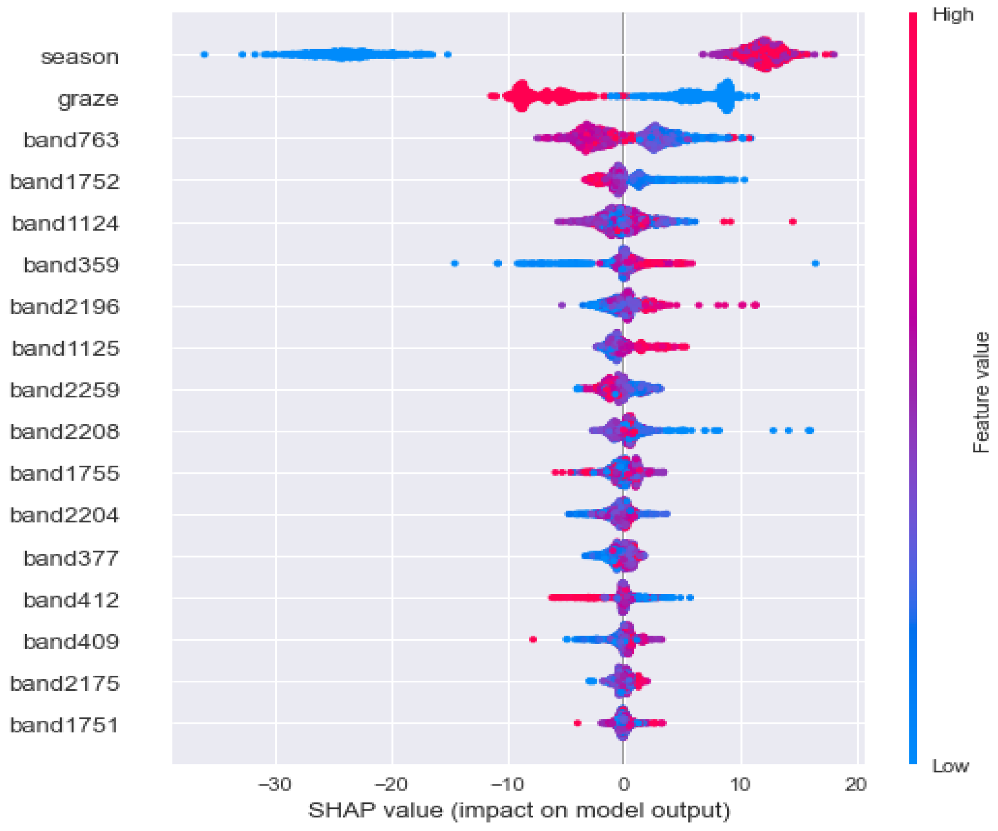
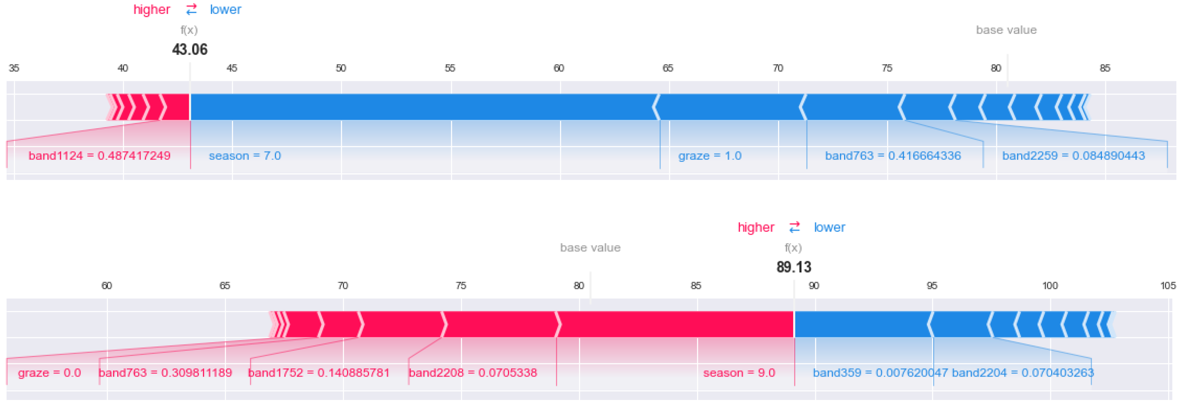
3.3.3. Interpretability of AGB Inversion Model Based on SHAP

Based on the results of the Lasso-GPR model in Table 3, SHAP was established for interpretability analysis.

(1)

The effect of features on AGB in aggregate data

Figure 16 mainly explains the difference between the output of the model and the base value of the model and which variables are responsible for the difference. Each point represents a sample (sample collected). The figure contains all samples. The X-axis represents the sorting result of samples according to the SHAP value. The Y-axis represents the sorting result of variables according to the SHAP value; the color represents the value of the variable. The larger the value of the variable, the redder the color, and the bluer the color. As an explanation of variables in the figure, season is the most important variable, and the larger the value (the redder the point), the higher the AGB (SHAP value > 0); graze was the second variable, in which no grazing had a positive effect on AGB, while grazing had a negative effect.

(2)

The influence of features on AGB in single data

The following figure (Figure 17) uses SHAP to visualize the influence of each feature in the article 40 data on AGB (restricted to the static graph display, only the feature with a large impact can be seen). The red feature indicates that AGB increases, and the blue feature indicates that AGB decreases. The increased or decreased data is the size of the SHAP value—that is, the width of each feature on the graph, where the f(x) (value is 43.06) at the red–blue line segment represents the AGB value of 43.06 g in this record, and the base value above the blue line segment on the right represents the AGB average value of all data. It can be clearly seen from left to right that (i) the value of band 1124 is about 0.487, resulting in an increase of 1.43 g in AGB; (ii) the season (July) with the value of 7 can explain the AGB reduction of 21 g; (iii) the graze score is 1 (grazing), indicating that AGB decreases by 7 g compared with no grazing. Under the combined action of all the characteristics, the AGB of the final record was much lower than the average, with seasonal factors, grazing factors, and band 763 having the greatest influence.

For comparison, article 800 data were selected for the same analysis. At this point, f(x) (value 89.13) at the red–blue line segment indicates that the AGB value in the record is 89.13 g, and the base value is located in the left red line segment. It can be seen from the figure that (i) when the graze score is 0 (no grazing), AGB increases by 2 g; (ii) Band 763, band 1752 and band 2208 explain the increase of 11 g AGB; (iii) the season with a value of 9 increases AGB; (iv) band 359 and band 2204 together reduce AGB by 9G. The record ended up with a slightly larger AGB than the average.

By comparing the two records, it can be found that the same band plays different roles in different records. For example, band 763 promotes the reduction of AGB in record 40, while it is opposite in record 800.

4. Discussion

The study’s findings reveal that for high-dimensional spectral datasets, each of the three feature selection algorithms exhibits its own set of properties (

Table 4. Comparison of advantages and disadvantages of three types of feature selection.

Models	Advantages	Disadvantages
Filter	Fast	Ignores interaction with the regression
	Scalable
Wrapper	Simple	Risk of overfitting
	Interacts with the regression	Model dependent
		Computationally intensive
Embedded	Interacts with the regression
	Less complexity than Wrapper	Model dependent

) [82,83,84]. Our findings show that the RFE_SVM-CHI or Lasso feature selection methods can significantly reduce the number of redundant variables and maximize useful feature variables; thus, the resulting variables can be confidently selected as important factors in the inversion of machine learning models. Not only does the optimal selection of variables have a stronger correlation to AGB, but it can also minimize the complexity of model training samples while enhancing prediction accuracy and capability. The feature selection algorithm, on the other hand, has several flaws. Although the R² and RMSE values of the models built using the Lasso and RFE_SVM approaches are fairly close, the variables screened by these two techniques are very different. To identify better variables, the similarities and differences between variable subsets must be further evaluated. In addition, we found that the results of the feature algorithm are not necessarily optimal. For example, we use the CHI algorithm to further process the results obtained by RFE_SVM, which can improve the effect on some models; that is, different feature selection algorithms can be combined to achieve the best goal.

In this study, we constructed a model based on diverse data and feature selection methods and tried to extract some knowledge about the relationship between spectral and ecological indicators from the AGB inversion of hyperspectral grassland. After creating multi-source data by incorporating grass height, growth season, and grazing condition factors, the model differs significantly from the pure spectral model. First, the applicability of the feature selection methods differed greatly from the findings of the algorithms. The MIC and RF feature selection algorithms converged too soon, picking only three variables and neglecting the importance of spectral variables. The Lasso and RFE_SVM approaches, on the other hand, added three variables in addition to retaining some spectral properties. This demonstrates that the spectrum can, to some extent, reflect the information contained in the three variables; however, not all feature selection techniques can do so. Second, a comparison of the machine learning inverse model outcomes demonstrates that adding at least one variable, i.e., the growing season, can produce excellent results, and adding three additional variables can make the model more resilient. This outcome allowed us to deduce the variables’ importance and function in this study. Finally, the spectra are utilized as a link between ecological experiments and remote sensing models to better comprehend the underlying mechanisms—it is much easier to conceptually grasp the model’s inherent meaning and ecological value than the typical inverted logic of merely creating mathematical models to enhance accuracy [85,86].

In the AGB inversion studied in this paper, the neural network-based deep learning regression model was roughly as effective as the optimal traditional machine learning regression model. Machine learning techniques are commonly applied in vegetation spectral surveys, and while they can efficiently solve for multiple covariates of the independent variables, the full validity of the models requires proper feature engineering. Deep learning models, however, combine feature extraction and performance evaluation to automatically perform optimal training. In general, of the two modeling approaches, deep learning models outperform machine learning models in terms of their statistical results and outperform elasticity and generalization models in terms of their predictive power [87,88]. However, after proper feature engineering, the results of machine learning and deep learning can be roughly the same, demonstrating the potential of the feature engineering approach. In addition, deep learning is a “black box”, and the “inside” of deep networks remains poorly understood [89]. Hyperparameters and network design are also conceptually challenging due to a lack of theoretical foundation [90].

Interpretability has always been a key and difficult problem in machine learning research. In the field of ecological remote sensing, we not only look forward to the improvement of results, but also hope that the model itself can provide new value for better understanding of nature. Some feature selection approaches adopted in this paper can determine the importance of different features, but we still do not know the specific role of features. By constructing an interpretable model based on SHAP, it can be found that SHAP values also evaluate features, which is different from the sorting and scoring of feature selection, and the distribution of features’ influence on samples (figure). It is even possible to analyze a single set of samples and visualize the different effects of each feature, reflecting the different effects of different samples, which is valuable for physiological analysis. However, the fundamental interpretability of spectra comes from the different responses of light at different wavelengths to different vegetation traits, which we have not studied.

Data–algorithm–model represents a trinity in data mining; however, in essence, both algorithm and model serve the data, which is thoroughly explored by continuously altering both the algorithm and model [91,92]. The data augment the supervised experience with prior information, the model reduces the size of the hypothesis space with prior knowledge, and the algorithm adjusts the search for the best hypothesis in a given hypothesis space with previous knowledge [93]. A major challenge in quantitative remote sensing inversion is that the applied parameters do not fully reflect the major elements affecting remote sensing information but merely produce weak indications of the underlying phenomena [30,94]. Although the inversion technique in data mining is more accurate, it also contains more parameters or hyperparameters and typically requires large-scale sophisticated training. The optimum algorithm should strike a balance between simulation accuracy, training parameters, and training duration. Using typical samples, excellent accuracy was achieved in this study. In a future study, we propose to tune the relevant machine learning parameters in terms of AGB and spectral response mechanism, better interpret the intrinsic connection between AGB and spectra, and establish a connection with existing multispectral remote sensing systems on this basis; we anticipate that the combination of these elements will provide a scientific basis for larger-scale AGB studies of alpine grasslands on the Tibetan plateau.

5. Conclusions

The results show that Lasso and RFE_SVM feature selection algorithms can quickly and accurately select feature spectra, effectively improving the representativeness and completeness of spectral analysis feature data, with the resulting model built based on the screened feature variables showing good predictive performance and high stamina. In the fields of feature variable screening and qualitative analysis, these algorithms have significant potential.

Machine learning with appropriate feature engineering reduces the training time of the AGB prediction model and greatly enhances its accuracy and predictive power, comparable to the performance of deep learning regression methods. When examining the impact of several data sources on the model, adding only seasons to the neural network prediction model results in higher accuracy; adding the other two components does not significantly improve the accuracy of the model, but it does improve its robustness.

The SHAP-based interpretable model gives the importance ranking of features and shows the role of feature population. At the same time, it can be found that the influence of the same feature in different records may be different; on the one hand, reflected in the direction of action (making the dependent variable increase or decrease), and on the other hand, reflected in the size.

References

1. Chen, Y.; Feng, J.; Yuan, X.; Zhu, B. Effects of warming on carbon and nitrogen cycling in alpine grassland ecosystems on the Tibetan Plateau: A meta-analysis. Geoderma 2020, 370, 114363. [Google Scholar] [CrossRef]
2. Chen, B.X.; Zhang, X.Z.; Tao, J.; Wu, J.S.; Wang, J.S.; Shi, P.L.; Zhang, Y.J.; Yu, C.Q. The impact of climate change and anthropogenic activities on alpine grassland over the Qinghai-Tibet Plateau. Agric. For. Meteorol. 2014, 189, 11–18. [Google Scholar] [CrossRef]
3. Conant, R.T.; Cerri, C.E.P.; Osborne, B.B.; Paustian, K. Grassland management impacts on soil carbon stocks: A new synthesis. Ecol. Appl. 2017, 27, 662–668. [Google Scholar] [CrossRef] [PubMed] [Green Version]
4. Fayiah, M.; Dong, S.K.; Khomera, S.W.; Rehman, S.A.U.; Yang, M.Y.; Xiao, J.N. Status and Challenges of Qinghai-Tibet Plateau’s Grasslands: An Analysis of Causes, Mitigation Measures, and Way Forward. Sustainability 2020, 12, 1099. [Google Scholar] [CrossRef] [Green Version]
5. Xiao, J.F.; Chevallier, F.; Gomez, C.; Guanter, L.; Hicke, J.A.; Huete, A.R.; Ichii, K.; Ni, W.J.; Pang, Y.; Rahman, A.F.; et al. Remote sensing of the terrestrial carbon cycle: A review of advances over 50 years. Remote Sens. Environ. 2019, 233, 37. [Google Scholar] [CrossRef]
6. Craven, D.; Eisenhauer, N.; Pearse, W.D.; Hautier, Y.; Isbell, F.; Roscher, C.; Bahn, M.; Beierkuhnlein, C.; Bonisch, G.; Buchmann, N.; et al. Multiple facets of biodiversity drive the diversity-stability relationship. Nat. Ecol. Evol. 2018, 2, 1579–1587. [Google Scholar] [CrossRef] [Green Version]
7. Isbell, F.; Calcagno, V.; Hector, A.; Connolly, J.; Harpole, W.S.; Reich, P.B.; Scherer-Lorenzen, M.; Schmid, B.; Tilman, D.; van Ruijven, J.; et al. High plant diversity is needed to maintain ecosystem services. Nature 2011, 477, 199–202. [Google Scholar] [CrossRef]
8. de Vries, F.T.; Griffiths, R.I.; Bailey, M.; Craig, H.; Girlanda, M.; Gweon, H.S.; Hallin, S.; Kaisermann, A.; Keith, A.M.; Kretzschmar, M.; et al. Soil bacterial networks are less stable under drought than fungal networks. Nat. Commun. 2018, 9, 12. [Google Scholar] [CrossRef] [Green Version]
9. Wagg, C.; Schlaeppi, K.; Banerjee, S.; Kuramae, E.E.; van der Heijden, M.G.A. Fungal-bacterial diversity and microbiome complexity predict ecosystem functioning. Nat. Commun. 2019, 10, 10. [Google Scholar] [CrossRef]
10. Morgan, J.A.; LeCain, D.R.; Pendall, E.; Blumenthal, D.M.; Kimball, B.A.; Carrillo, Y.; Williams, D.G.; Heisler-White, J.; Dijkstra, F.A.; West, M. C-4 grasses prosper as carbon dioxide eliminates desiccation in warmed semi-arid grassland. Nature 2011, 476, 202–205. [Google Scholar] [CrossRef]
11. Dong, S.K.; Shang, Z.H.; Gao, J.X.; Boone, R.B. Enhancing sustainability of grassland ecosystems through ecological restoration and grazing management in an era of climate change on Qinghai-Tibetan Plateau. Agric. Ecosyst. Environ. 2020, 287, 16. [Google Scholar] [CrossRef]
12. Wang, G.X.; Li, Y.S.; Wang, Y.B.; Wu, Q.B. Effects of permafrost thawing on vegetation and soil carbon pool losses on the Qinghai-Tibet Plateau, China. Geoderma 2008, 143, 143–152. [Google Scholar] [CrossRef]
13. Yang, Y.; Tilman, D.; Furey, G.; Lehman, C. Soil carbon sequestration accelerated by restoration of grassland biodiversity. Nat. Commun. 2019, 10, 7. [Google Scholar] [CrossRef] [PubMed] [Green Version]
14. Bosch, A.; Dorfer, C.; He, J.S.; Schmidt, K.; Scholten, T. Predicting soil respiration for the Qinghai-Tibet Plateau: An empirical comparison of regression models. Pedobiologia 2016, 59, 41–49. [Google Scholar] [CrossRef]
15. Veldhuis, M.P.; Ritchie, M.E.; Ogutu, J.O.; Morrison, T.A.; Beale, C.M.; Estes, A.B.; Mwakilema, W.; Ojwang, G.O.; Parr, C.L.; Probert, J.; et al. Cross-boundary human impacts compromise the Serengeti-Mara ecosystem. Science 2019, 363, 1424–1428. [Google Scholar] [CrossRef] [PubMed] [Green Version]
16. Wang, L.; Delgado-Baquerizo, M.; Wang, D.L.; Isbell, F.; Liu, J.; Feng, C.; Liu, J.S.; Zhong, Z.W.; Zhu, H.; Yuan, X.; et al. Diversifying livestock promotes multidiversity and multifunctionality in managed grasslands. Proc. Natl. Acad. Sci. USA 2019, 116, 6187–6192. [Google Scholar] [CrossRef] [Green Version]
17. Liu, H.Y.; Mi, Z.R.; Lin, L.; Wang, Y.H.; Zhang, Z.H.; Zhang, F.W.; Wang, H.; Liu, L.L.; Zhu, B.A.; Cao, G.M.; et al. Shifting plant species composition in response to climate change stabilizes grassland primary production. Proc. Natl. Acad. Sci. USA 2018, 115, 4051–4056. [Google Scholar] [CrossRef] [Green Version]
18. Miehe, G.; Schleuss, P.M.; Seeber, E.; Babel, W.; Biermann, T.; Braendle, M.; Chen, F.H.; Coners, H.; Foken, T.; Gerken, T.; et al. The Kobresia pygmaea ecosystem of the Tibetan highlands—Origin, functioning and degradation of the world’s largest pastoral alpine ecosystem Kobresia pastures of Tibet. Sci. Total Environ. 2019, 648, 754–771. [Google Scholar] [CrossRef]
19. Lemaire, G.; Franzluebbers, A.; Carvalho, P.C.D.; Dedieu, B. Integrated crop-livestock systems: Strategies to achieve synergy between agricultural production and environmental quality. Agric. Ecosyst. Environ. 2014, 190, 4–8. [Google Scholar] [CrossRef]
20. Reinermann, S.; Asam, S.; Kuenzer, C. Remote Sensing of Grassland Production and Management-A Review. Remote Sens. 2020, 12, 1949. [Google Scholar] [CrossRef]
21. Kumar, L.; Sinha, P.; Taylor, S.; Alqurashi, A.F. Review of the use of remote sensing for biomass estimation to support renewable energy generation. J. Appl. Remote Sens. 2015, 9, 28. [Google Scholar] [CrossRef]
22. Eisfelder, C.; Kuenzer, C.; Dech, S. Derivation of biomass information for semi-arid areas using remote-sensing data. Int. J. Remote Sens. 2012, 33, 2937–2984. [Google Scholar] [CrossRef]
23. Wachendorf, M.; Fricke, T.; Moeckel, T. Remote sensing as a tool to assess botanical composition, structure, quantity and quality of temperate grasslands. Grass Forage Sci. 2018, 73, 1–14. [Google Scholar] [CrossRef]
24. Liang, T.; Yang, S.; Feng, Q.; Liu, B.; Zhang, R.; Huang, X.; Xie, H. Multi-factor modeling of above-ground biomass in alpine grassland: A case study in the Three-River Headwaters Region, China. Remote Sens. Environ. 2016, 186, 164–172. [Google Scholar] [CrossRef]
25. Pang, H.; Zhang, A.; Kang, X.; He, N.; Dong, G. Estimation of the Grassland Aboveground Biomass of the Inner Mongolia Plateau Using the Simulated Spectra of Sentinel-2 Images. Remote Sens. 2020, 12, 4155. [Google Scholar] [CrossRef]
26. Sun, S.; Wang, C.; Yin, X.; Wang, W.; Liu, W.; Zhang, Y.; Zhao, Q.Z. Estimating aboveground biomass of natural grassland based on multispectral images of Unmanned Aerial Vehicles. J. Remote Sens. 2018, 22, 848–856. [Google Scholar] [CrossRef]
27. Khaliq, A.; Comba, L.; Biglia, A.; Aimonino, D.R.; Chiaberge, M.; Gay, P. Comparison of Satellite and UAV-Based Multispectral Imagery for Vineyard Variability Assessment. Remote Sens. 2019, 11, 436. [Google Scholar] [CrossRef] [Green Version]
28. Tattaris, M.; Reynolds, M.P.; Chapman, S.C. A Direct Comparison of Remote Sensing Approaches for High-Throughput Phenotyping in Plant Breeding. Front. Plant Sci. 2016, 7, 1131. [Google Scholar] [CrossRef]
29. Transon, J.; d’Andrimont, R.; Maugnard, A.; Defourny, P. Survey of Hyperspectral Earth Observation Applications from Space in the Sentinel-2 Context. Remote Sens. 2018, 10, 157. [Google Scholar] [CrossRef] [Green Version]
30. van der Meer, F.D.; van der Werff, H.M.A.; van Ruitenbeek, F.J.A.; Hecker, C.A.; Bakker, W.H.; Noomen, M.F.; van der Meijde, M.; Carranza, E.J.M.; de Smeth, J.B.; Woldai, T. Multi- and hyperspectral geologic remote sensing: A review. Int. J. Appl. Earth Obs. Geoinf. 2012, 14, 112–128. [Google Scholar] [CrossRef]
31. Shi, Y.; Gao, J.; Li, X.; Li, J.; dela Torre, D.M.G.; Brierley, G.J. Improved Estimation of Aboveground Biomass of Disturbed Grassland through Including Bare Ground and Grazing Intensity. Remote Sens. 2021, 13, 2015. [Google Scholar] [CrossRef]
32. Melville, B.; Lucieer, A.; Aryal, J. Assessing the Impact of Spectral Resolution on Classification of Lowland Native Grassland Communities Based on Field Spectroscopy in Tasmania, Australia. Remote Sens. 2018, 10, 308. [Google Scholar] [CrossRef] [Green Version]
33. Oberrneier, W.A.; Lehnert, L.W.; Pohl, M.J.; Gianonni, S.M.; Silva, B.; Seibert, R.; Laser, H.; Moser, G.; Muller, C.; Luterbacher, J.; et al. Grassland ecosystem services in a changing environment: The potential of hyperspectral monitoring. Remote Sens. Environ. 2019, 232, 16. [Google Scholar] [CrossRef]
34. Wang, J.; Brown, D.G.; Bai, Y.F. Investigating the spectral and ecological characteristics of grassland communities across an ecological gradient of the Inner Mongolian grasslands with in situ hyperspectral data. Int. J. Remote Sens. 2014, 35, 7179–7198. [Google Scholar] [CrossRef]
35. Shahshahani, B.M.; Landgrebe, D.A. The effect of unlabeled samples in reducing the small sample-size problem and mitigating the hughes phenomenon. IEEE Trans. Geosci. Remote Sens. 1994, 32, 1087–1095. [Google Scholar] [CrossRef] [Green Version]
36. Taskin, G.; Kaya, H.; Bruzzone, L. Feature Selection Based on High Dimensional Model Representation for Hyperspectral Images. IEEE Trans. Image Process. 2017, 26, 2918–2928. [Google Scholar] [CrossRef]
37. Fava, F.; Parolo, G.; Colombo, R.; Gusmeroli, F.; Della Marianna, G.; Monteiro, A.T.; Bocchi, S. Fine-scale assessment of hay meadow productivity and plant diversity in the European Alps using field spectrometric data. Agric. Ecosyst. Environ. 2010, 137, 151–157. [Google Scholar] [CrossRef]
38. Marabel, M.; Alvarez-Taboada, F. Spectroscopic Determination of Aboveground Biomass in Grasslands Using Spectral Transformations, Support Vector Machine and Partial Least Squares Regression. Sensors 2013, 13, 10027–10051. [Google Scholar] [CrossRef] [Green Version]
39. Bratsch, S.; Epstein, H.; Buchhorn, M.; Walker, D.; Landes, H. Relationships between hyperspectral data and components of vegetation biomass in Low Arctic tundra communities at Ivotuk, Alaska. Environ. Res. Lett. 2017, 12, 14. [Google Scholar] [CrossRef]
40. Chandrashekar, G.; Sahin, F. A survey on feature selection methods. Comput. Electr. Eng. 2014, 40, 16–28. [Google Scholar] [CrossRef]
41. Brown, L.G. A SURVEY OF Image registration techniques. Comput. Surv. 1992, 24, 325–376. [Google Scholar] [CrossRef]
42. Shen, M.; Tang, Y.; Klein, J.; Zhang, P.; Gu, S.; Shimono, A.; Chen, J. Estimation of aboveground biomass using in situ hyperspectral measurements in five major grassland ecosystems on the Tibetan Plateau. J. Plant Ecol. 2008, 1, 247–257. [Google Scholar] [CrossRef] [Green Version]
43. Gao, J.X.; Chen, Y.M.; Lu, S.H.; Feng, C.Y.; Chang, X.L.; Ye, S.X.; Liu, J.D. A ground spectral model for estimating biomass at the peak of the growing season in Hulunbeier grassland, Inner Mongolia, China. Int. J. Remote Sens. 2012, 33, 4029–4043. [Google Scholar] [CrossRef]
44. Ali, I.; Greifeneder, F.; Stamenkovic, J.; Neumann, M.; Notarnicola, C. Review of Machine Learning Approaches for Biomass and Soil Moisture Retrievals from Remote Sensing Data. Remote Sens. 2015, 7, 16398–16421. [Google Scholar] [CrossRef] [Green Version]
45. Dargan, S.; Kumar, M.; Ayyagari, M.R.; Kumar, G. A Survey of Deep Learning and Its Applications: A New Paradigm to Machine Learning. Arch. Comput. Method Eng. 2020, 27, 1071–1092. [Google Scholar] [CrossRef]
46. Su, J.W.; Vargas, D.V.; Sakurai, K. One Pixel Attack for Fooling Deep Neural Networks. IEEE Trans. Evol. Comput. 2019, 23, 828–841. [Google Scholar] [CrossRef] [Green Version]
47. Arrieta, A.B.; Diaz-Rodriguez, N.; Del Ser, J.; Bennetot, A.; Tabik, S.; Barbado, A.; Garcia, S.; Gil-Lopez, S.; Molina, D.; Benjamins, R.; et al. Explainable Artificial Intelligence (XAI): Concepts, taxonomies, opportunities and challenges toward responsible AI. Inf. Fusion 2020, 58, 82–115. [Google Scholar] [CrossRef] [Green Version]
48. McGovern, A.; Lagerquist, R.; Gagne, D.J.; Jergensen, G.E.; Elmore, K.L.; Homeyer, C.R.; Smith, T. Making the Black Box More Transparent: Understanding the Physical Implications of Machine Learning. Bull. Amer. Meteorol. Soc. 2019, 100, 2175–2199. [Google Scholar] [CrossRef]
49. ASD Inc. FieldSpec®4 UserManual. Available online: http://support.asdi.com/Document/FileGet.aspx?f=600000.PDF (accessed on 10 December 2015).
50. Curra, A.; Gasbarrone, R.; Cardillo, A.; Trompetto, C.; Fattapposta, F.; Pierelli, F.; Missori, P.; Bonifazi, G.; Serranti, S. Near-infrared spectroscopy as a tool for in vivo analysis of human muscles. Sci Rep 2019, 9, 14. [Google Scholar] [CrossRef]
51. Steinier, J.; Termonia, Y.; Deltour, J. Smoothing and differentiation of data by simplified least square procedure. Anal. Chem. 1972, 44, 1906–1909. [Google Scholar] [CrossRef]
52. Li, J.D.; Cheng, K.W.; Wang, S.H.; Morstatter, F.; Trevino, R.P.; Tang, J.L.; Liu, H. Feature Selection: A Data Perspective. ACM Comput. Surv. 2018, 50, 45. [Google Scholar] [CrossRef] [Green Version]
53. Gui, J.; Sun, Z.N.; Ji, S.W.; Tao, D.C.; Tan, T.N. Feature Selection Based on Structured Sparsity: A Comprehensive Study. IEEE Trans. Neural Netw. Learn. Syst. 2017, 28, 1490–1507. [Google Scholar] [CrossRef] [PubMed]
54. Cai, J.; Luo, J.W.; Wang, S.L.; Yang, S. Feature selection in machine learning: A new perspective. Neurocomputing 2018, 300, 70–79. [Google Scholar] [CrossRef]
55. Lazar, C.; Taminau, J.; Meganck, S.; Steenhoff, D.; Coletta, A.; Molter, C.; de Schaetzen, V.; Duque, R.; Bersini, H.; Nowe, A. A Survey on Filter Techniques for Feature Selection in Gene Expression Microarray Analysis. IEEE-ACM Trans. Comput. Biol. Bioinform. 2012, 9, 1106–1119. [Google Scholar] [CrossRef] [PubMed]
56. McHugh, M.L. The Chi-square test of independence. Biochem. Medica. 2013, 23, 143–149. [Google Scholar] [CrossRef] [PubMed] [Green Version]
57. Austin, P.C.; Steyerberg, E.W. The number of subjects per variable required in linear regression analyses. J. Clin. Epidemiol. 2015, 68, 627–636. [Google Scholar] [CrossRef] [Green Version]
58. Chu, F.C.; Fan, Z.P.; Guo, B.H.; Zhi, D.; Yin, Z.J.; Zhao, W.J. Variable Selection based on Maximum Information Coefficient for Data Modeling. In Proceedings of the 2nd IEEE Advanced Information Technology, Electronic and Automation Control Conference (IAEAC), Chongqing, China, 25–26 March 2017; pp. 1714–1717. [Google Scholar]
59. Kohavi, R.; John, G.H. Wrappers for feature subset selection. Artif. Intell. 1997, 97, 273–324. [Google Scholar] [CrossRef] [Green Version]
60. Mao, Y.; Pi, D.Y.; Liu, Y.M.; Sun, Y.X. Accelerated recursive feature elimination based on support vector machine for key variable identification. Chin. J. Chem. Eng. 2006, 14, 65–72. [Google Scholar] [CrossRef]
61. Zhang, R.; Ma, J.W.; Chen, X.; Tong, Q.X. Feature selection for hyperspectral data based on modified recursive support vector machines. In Proceedings of the IEEE International Geoscience and Remote Sensing Symposium, Cape Town, South Africa, 12–17 July 2009; pp. II-847–II-850. [Google Scholar]
62. Zhang, X.C.; Zhao, Z.X.; Zheng, Y.; Li, J.Y. Prediction of Taxi Destinations Using a Novel Data Embedding Method and Ensemble Learning. IEEE Trans. Intell. Transp. Syst. 2020, 21, 68–78. [Google Scholar] [CrossRef]
63. Xia, J.N.; Sun, D.Y.; Xiao, F. Summary of lasso and relative methods. In Proceedings of the 13th International Conference on Enterprise Information Systems (ICEIS 2011), Beijing, China, 8–11 June 2011; Beijing Jiaotong University, Sch Econ & Management: Beijing, China, 2011; pp. 131–134. [Google Scholar]
64. Jain, R.H.; Xu, W. HDSI: High dimensional selection with interactions algorithm on feature selection and testing. PLoS ONE 2021, 16, 17. [Google Scholar] [CrossRef]
65. Dormann, C.F.; Elith, J.; Bacher, S.; Buchmann, C.; Carl, G.; Carre, G.; Marquez, J.R.G.; Gruber, B.; Lafourcade, B.; Leitao, P.J.; et al. Collinearity: A review of methods to deal with it and a simulation study evaluating their performance. Ecography 2013, 36, 27–46. [Google Scholar] [CrossRef]
66. Muthukrishnan, R.; Rohini, R. LASSO: A Feature Selection Technique In Predictive Modeling For Machine Learning. In Proceedings of the IEEE International Conference on Advances in Computer Applications (ICACA), Coimbatore, India, 24 October 2016; pp. 18–20. [Google Scholar]
67. Verikas, A.; Gelzinis, A.; Bacauskiene, M. Mining data with random forests: A survey and results of new tests. Pattern Recognit. 2011, 44, 330–349. [Google Scholar] [CrossRef]
68. Belgiu, M.; Dragut, L. Random forest in remote sensing: A review of applications and future directions. ISPRS-J. Photogramm. Remote Sens. 2016, 114, 24–31. [Google Scholar] [CrossRef]
69. Hearst, M.A. Support vector machines. IEEE Intell. Syst. Appl. 1998, 13, 18–21. [Google Scholar] [CrossRef] [Green Version]
70. Mountrakis, G.; Im, J.; Ogole, C. Support vector machines in remote sensing: A review. ISPRS-J. Photogramm. Remote Sens. 2011, 66, 247–259. [Google Scholar] [CrossRef]
71. Schulz, E.; Speekenbrink, M.; Krause, A. A tutorial on Gaussian process regression: Modelling, exploring, and exploiting functions. J. Math. Psychol. 2018, 85, 1–16. [Google Scholar] [CrossRef]
72. Williams, C.; Rasmussen, C. Gaussian processes for regression. In Proceedings of the Advances in Neural Information Processing Systems 8, Denver, CO, USA, 27–30 November 1995. [Google Scholar]
73. Liu, H.T.; Ong, Y.S.; Shen, X.B.; Cai, J.F. When Gaussian Process Meets Big Data: A Review of Scalable GPs. IEEE Trans. Neural Netw. Learn. Syst. 2020, 31, 4405–4423. [Google Scholar] [CrossRef] [PubMed] [Green Version]
74. Ambikasaran, S.; Foreman-Mackey, D.; Greengard, L.; Hogg, D.W.; O’Neil, M. Fast Direct Methods for Gaussian Processes. IEEE Trans. Pattern Anal. Mach. Intell. 2016, 38, 252–265. [Google Scholar] [CrossRef] [Green Version]
75. Hastie, T.; Tibshirani, R.; Friedman, J.H.; Friedman, J.H. The Elements of Statistical Learning: Data Mining, Inference, and Prediction, 2nd ed.; Spring: New York, NY, USA, 2008. [Google Scholar]
76. Abu-Taieh, E.M. Artificial neural networks: Enhanced Back Propagation in character recognition. In Proceedings of the International Conference of the Information-Resources-Management-Association, Philadelphia, PA, USA, 18–21 May 2003; pp. 263–265. [Google Scholar]
77. Rumelhart, D.E.; Hinton, G.E.; Williams, R.J.J.N. Learning Representations by Back Propagating Errors. Nature 1986, 323, 533–536. [Google Scholar] [CrossRef]
78. Pedregosa, F.; Varoquaux, G.; Gramfort, A.; Michel, V.; Thirion, B.; Grisel, O.; Blondel, M.; Prettenhofer, P.; Weiss, R.; Dubourg, V.; et al. Scikit-learn: Machine Learning in Python. J. Mach. Learn. Res. 2011, 12, 2825–2830. [Google Scholar]
79. Sharma, P.; Mirzan, S.R.; Bhandari, A.; Pimpley, A.; Eswaran, A.; Srinivasan, S.; Shao, L.Q. Evaluating Tree Explanation Methods for Anomaly Reasoning: A Case Study of SHAP TreeExplainer and TreeInterpreter. In Proceedings of the 39th International Conference on Conceptual Modeling (ER), Vienna, Austria, 3–6 November 2020; pp. 35–45. [Google Scholar]
80. Nohara, Y.; Matsumoto, K.; Soejima, H.; Nakashima, N. Explanation of machine learning models using shapley additive explanation and application for real data in hospital. Comput. Meth. Progr. Biomed. 2022, 214, 6. [Google Scholar] [CrossRef] [PubMed]
81. Li, Z.M.; Zhang, Q.; Du, X.Y.; Ma, Y.F.; Wang, S.H. Social media rumor refutation effectiveness: Evaluation, modelling and enhancement. Inf. Processing Manag. 2021, 58, 102420. [Google Scholar] [CrossRef]
82. Zhiqin, L. Summary of feature selection methods. Comput. Eng. Appl. 2019, 55, 10–19. [Google Scholar] [CrossRef]
83. Chaofang, L. The Research on Causal Feature Selection Algorithm Based on AD-Tree; Hefei University of Technology: Hefei, China, 2021; pp. 7–9. [Google Scholar] [CrossRef]
84. Ruiqi, J. Research on Interpretable Prediction Model of Traumatic Hemorrhagic Shock Based on Improved ANN; Beijing Jiaotong University: Beijing, China, 2021; pp. 13–16. [Google Scholar] [CrossRef]
85. Wu, J.; Peng, D.L. Advances in Researches on Hyperspectral Remote Sensing Forestry Information-Extracting Technology. Spectrosc. Spectr. Anal. 2011, 31, 2305–2312. [Google Scholar] [CrossRef]
86. Smith, W.K.; Dannenberg, M.P.; Yan, D.; Herrmann, S.; Barnes, M.L.; Barron-Gafford, G.A.; Biederman, J.A.; Ferrenberg, S.; Fox, A.M.; Hudson, A.; et al. Remote sensing of dryland ecosystem structure and function: Progress, challenges, and opportunities. Remote Sens. Environ. 2019, 233, 23. [Google Scholar] [CrossRef]
87. Long, W.; Lu, Z.C.; Cui, L.X. Deep learning-based feature engineering for stock price movement prediction. Knowl.-Based Syst. 2019, 164, 163–173. [Google Scholar] [CrossRef]
88. Sagheer, A.; Kotb, M. Time series forecasting of petroleum production using deep LSTM recurrent networks. Neurocomputing 2019, 323, 203–213. [Google Scholar] [CrossRef]
89. Li, T.Y.; Fong, S.M.; Siu, S.W.I.; Yang, X.S.; Liu, L.S.; Mohammed, S. White learning methodology: A case study of cancer-related disease factors analysis in real-time PACS environment. Comput. Meth. Programs Biomed. 2020, 197, 18. [Google Scholar] [CrossRef]
90. Pouyanfar, S.; Sadiq, S.; Yan, Y.L.; Tian, H.M.; Tao, Y.D.; Reyes, M.P.; Shyu, M.L.; Chen, S.C.; Iyengar, S.S. A Survey on Deep Learning: Algorithms, Techniques, and Applications. ACM Comput. Surv. 2019, 51, 36. [Google Scholar] [CrossRef]
91. Kalaba, R.E.; Johnson, J.; Natsuyama, H.H. Statistical measures for least squares using the alpha Q beta R algorithm. J. Optim. Theory Appl. 2005, 127, 515–522. [Google Scholar] [CrossRef]
92. Wu, X.D.; Zhu, X.Q.; Wu, G.Q.; Ding, W. Data Mining with Big Data. IEEE Trans. Knowl. Data Eng. 2014, 26, 97–107. [Google Scholar] [CrossRef]
93. Wang, Y.Q.; Yao, Q.M.; Kwok, J.T.; Ni, L.M. Generalizing from a Few Examples: A Survey on Few-shot Learning. ACM Comput. Surv. 2020, 53, 34. [Google Scholar] [CrossRef]
94. Aasen, H.; Honkavaara, E.; Lucieer, A.; Zarco-Tejada, P.J. Quantitative Remote Sensing at Ultra-High Resolution with UAV Spectroscopy: A Review of Sensor Technology, Measurement Procedures, and Data Correction Workflows. Remote Sens. 2018, 10, 1091. [Google Scholar] [CrossRef] [Green Version]
Figure 1. Overview of the study area. (a) Digital elevation model (DEM) map of Qinghai Province, China, where the study area is located. (b) A drone view of the test site. Image bands are red, green, and blue. Ten of the sample plots were enclosed, while the other ten were allowed to be freely grazed.
Remotesensing 14 02086 g001
Figure 2. Three different feature selection schematics. (a) Filter feature selection; (b) wrapped feature selection; (c) embedded feature selection.
Remotesensing 14 02086 g002
Figure 3. Interpretability framework based on SHAP values.
Remotesensing 14 02086 g003
Figure 4. AGB inversion data processing course.
Remotesensing 14 02086 g004
Figure 5. Histogram of the overall AGB sample. The red circle indicates a maximum AGB of 220 g.
Remotesensing 14 02086 g005
Figure 6. Box plots showing statistical analysis of AGB and grass height by month (7 = July, 8 = August, 9 = September). Numbers 0 and 1 indicate not grazed and grazed.
Remotesensing 14 02086 g006aRemotesensing 14 02086 g006b
Figure 7. Scatter plot of AGB and grass height.
Remotesensing 14 02086 g007
Figure 8. Field measured spectral curves. The Max line is the highest reflectivity hyperspectral. The Min line is the lowest reflectivity hyperspectral curve. The Mean line shows the mean and variance of the spectrum.
Remotesensing 14 02086 g008
Figure 9. Results of feature scoring based on spectral data. The abscissa is the feature number and the ordinate is the score. MEAN shows the average value of all algorithms.
Remotesensing 14 02086 g009
Figure 10. Results of feature selection based on spectral data.
Remotesensing 14 02086 g010
Figure 11. Feature scoring based on multi-source data. The abscissa is the feature number, and the ordinate is the score.
Remotesensing 14 02086 g011
Figure 12. Feature selection results based on multi-source data.
Remotesensing 14 02086 g012
Figure 13. Feature selection results of four RFE_SVM algorithms.
Remotesensing 14 02086 g013
Figure 14. Neural network structure.
Remotesensing 14 02086 g014
Figure 15. AGB inversion results of different data sources. (a) Spectral data only; (b) spectral data and seasons; (c) combining spectrum, season, grass height; (d) combining spectrum, season, grass height, grazing situation.
Remotesensing 14 02086 g015aRemotesensing 14 02086 g015b
Figure 16. AGB inversion data processing process.
Remotesensing 14 02086 g016
Figure 17. AGB inversion data processing process. The top chart shows article 40 data and the bottom chart shows article 800 data.
Remotesensing 14 02086 g017