Article

Hyperspectral Image Mixed Noise Removal Using a Subspace Projection Attention and Residual Channel Attention Network

1
Research Center of Satellite Technology, Harbin Institute of Technology, Harbin 150001, China
2
China Academy of Space Technology, Beijing 100094, China
3
Key Laboratory of Computational Optical Imaging Technology, Aerospace Information Research Institute, Chinese Academy of Sciences, Beijing 100094, China
4
College of Geography and Environment, Liaocheng University, Liaocheng 252059, China
5
Research Center for Space Optical Engineering, Harbin Institute of Technology, Harbin 150001, China
*
Author to whom correspondence should be addressed.
Remote Sens. 2022, 14(9), 2071; https://doi.org/10.3390/rs14092071
Submission received: 24 March 2022 / Revised: 15 April 2022 / Accepted: 22 April 2022 / Published: 26 April 2022
(This article belongs to the Special Issue Pattern Recognition in Hyperspectral Remote Sensing)

Abstract

:
Although the existing deep-learning-based hyperspectral image (HSI) denoising methods have achieved tremendous success, recovering high-quality HSIs in complex scenes that contain mixed noise is still challenging. Besides, these methods have not fully explored the local and global spatial–spectral information of HSIs. To address the above issues, a novel HSI mixed noise removal network called subspace projection attention and residual channel attention network (SPARCA-Net) is proposed. Specifically, we propose an orthogonal subspace projection attention (OSPA) module to adaptively learn to generate bases of the signal subspace and project the input into such space to remove noise. By leveraging the local and global spatial relations, OSPA is able to reconstruct the local structure of the feature maps more precisely. We further propose a residual channel attention (RCA) module to emphasize the interdependence between feature maps and exploit the global channel correlation of them, which could enhance the channel-wise adaptive learning. In addition, multiscale joint spatial–spectral input and residual learning strategies are employed to capture multiscale spatial–spectral features and reduce the degradation problem, respectively. Synthetic and real HSI data experiments demonstrated that the proposed HSI denoising network outperforms many of the advanced methods in both quantitative and qualitative assessments.

Graphical Abstract

1. Introduction

Hyperspectral remote sensing is a technology that acquires multidimensional information, which combines imaging and spectroscopy technologies, and its data contain both two-dimensional geometric spatial information and one-dimensional spectral information of ground objects. Hyperspectral imaging typically records the spectral information in a series of continuous channels, which generally have a narrow spectral bandwidth (for example, usually below 10 nm); therefore, hyperspectral images (HSIs) contain the fine spectral characteristics of the targets [1,2,3]. With the high-dimensional and distinguishing spectral features, HSIs have been widely used in many applications [4,5,6,7,8].
HSI is a three-dimensional data cube, generally including hundreds of bands. With the decrease in the width of spectral bands, the detector imaging system receives fewer photons per band, thus introducing complex noise, such as random noise and structural stripe noise and deadlines; the existence of mixed noise not only significantly affects the images’ signal-to-noise ratio (SNR) but also degrades the spectral signature quality, thus affecting the subsequent information extraction [9,10]. Therefore, denoising is a crucial preprocessing step before HSIs can be further applied [11,12], and researchers have presented many HSI denoising methods in the past few decades.
Spatial-Domain-Based Methods. The spatial-domain-based denoising method usually regards the three-dimensional hyperspectral image as an extension of the RGB image and applies the traditional two-dimensional denoising algorithms to denoise the hyperspectral image band by band. Such methods can be categorized into pixel-space-based methods and transform-domain-space-based methods. The former one does not perform any transformation on the pixel value, and it directly performs the denoising operation. The typical algorithms are the non-local mean (NLM) algorithm [13], Bayes algorithm [14], bilateral filtering [15] and denoising methods based on sparse and redundant representations [16], etc. These types of methods are easy to operate and implement, but there are limitations in practical applications, and the effect of removing severe noise is not good. The method based on the transform domain uses the difference in a specific transform domain between the original image and the noise to separate the main signal and the noise. Commonly used specific transform domains are wavelet transform domain and Fourier transform domain. Representative examples of this methodology include adaptive wavelet thresholding [17], block-matching and 3D filtering (BM3D) [18], the extending of BM3D to multiband image denoising and block-matching and 4D filtering (BM4D) [19]. However, the spatial-domain-based denoising methods ignore the correlation between the bands and only have a certain effect for a specific type of noise and thus cannot deal with the mixed noise problem.
Spectral-Domain-Based Methods. HSIs contain numerous information in hundreds of bands. Therefore, in addition to the above spatial-domain-based denoising methods, the spectral-domain information of HSIs can also be used for denoising. Green et al. [20] used maximum noise fraction (MNF) transform to remove noise. Donoho et al. [21] proposed a SureShrink algorithm via wavelet transform of the spectral domain signal. The spectral-domain-based denoising methods were proposed from the perspective of signal processing and ignore spatial structure information, which is likely to cause spatial pixel distortion, resulting in limited image restoration effects.
Prior-Constraint-Based Methods. Denoising methods based on the spatial domain and the spectral domain could remove certain specific noises, such as Gaussian noise, but these two types of methods only use spatial or spectral information, making the effect of removing mixed noises poor. The denoising method based on prior constraint could make full use of the information in the spatial and spectral domains and has become one of the hot topics and trends in the field of remote sensing images. This method transforms the denoising problem into a prior constraint problem. The prior constraints of remote sensing images directly determine the restoration effect. The low rankness of HSIs in the spectral dimension is a widely used image prior in an HSI denoising task. Representative low-rankness-based methods include, for example, PCA (principal components analysis) [22], LRTA (low-rank tensor approximation) [23], LRTR (low-rank tensor recovery) [24], LRMR (low-rank matrix recovery) [25], NAILRMA (noise-adjusted iterative low-rank matrix approximation) [26], BLRMF (bilinear low-rank matrix factorization) [27], NLR-CPTD (nonlocal low-rank regularized CP tensor decomposition) [28] and so on. Total variation is also a widely used image prior in regard to a denoising problem. Some total-variation-based methods are, for example, SSAHTV (spectral–spatial adaptive total variation) [29], SSTV (spatio-spectral total variation) [30], E3DTV (enhanced-3DTV) [31], etc. Recently, researchers combined low-rank constraints with total variation constraints and have proposed many HSI denoising methods [32,33,34,35]. In summary, the HSI denoising methods based on prior constraints exploit the low-rank and spatial–spectral structure information of HSIs and achieve meaningful results. The subspace representation of spectral vectors in HSIs has been successfully used to remove noise by regularizing the representation coefficients of HSIs, such as FastHyDe (fast hyperspectral denoising) [36], NGmeet (non-local meets global) [37], L1HyMixDe [38], etc.
Deep-Learning-Based Methods. Although the above methods can achieve good results, the models of such are fixed and the parameters should be tuned precisely, so the methods may be unstable and sensitive to the data [39]. In recent years, deep learning (DL) has demonstrated better performance than traditional methods in many computer vision tasks [40,41,42,43] and has also been introduced into HSI processing, including fusion [44], unmixing [45,46,47], data enhancement [48] and so on. DL-based denoising methods usually employ supervised models, which take clean and noisy image pairs as the inputs and train the network to learn the prior distribution of clean images, thereby establishing an end-to-end mapping from noisy images to clean images. For the HSI denoising task, the exploration of the combination of spatial and spectral information, the extraction and representation of the features of HSI are the focus of the researchers. For Gaussian noise, Yuan et al. [49] used the spatial band and its adjacent bands as inputs for the model to extract features while introducing multiscale convolution layers to extract multiscale features in spatial and spectral dimensions. Chang et al. [48] proposed the HSI-DeNet, which applied a residual learning strategy, dilated convolution and multichannel filtering and achieved great performance for mixed noise denoising. Zhang et al. [50] proposed a spatial–spectral gradient network (SSGN), which employed a spatial–spectral gradient learning strategy, taking a single band, its horizontal/vertical spatial gradient images and its adjacent spectral gradient as inputs considering that sparse noise is spatially directional and the spectral gradient is used as additional supplementary information. Moreover, recently, some work based on the attention mechanism [39,51,52] has been proposed. Although the existing DL-based HSI denoising methods have achieved great success, recovering high-quality HSIs in difficult scenes, such as severe noise and mixed noise, is still challenging. In addition, these methods still do not fully exploit the local and global spatial–spectral prior information of the HSI because, usually, the convolution operation only exploits the local spatial and spectral prior information of the HSI.
To address the above problems, a novel subspace projection attention and residual channel attention network (SPARCA-Net) for HSI denoising is proposed. Specifically, the proposed model takes a single band and its adjacent bands’ images as the inputs, and two attention-based modules are proposed to exploit the global prior information in spatial and spectral domains. Firstly, from the perspective of adaptive projection and reconstruction, an orthogonal subspace projection attention (OSPA) module is proposed to adaptively learn to generate a set of orthogonal subspace bases; the main signal of shallow feature maps can be enhanced after projecting the shallow feature maps into subspace for facilitating separation from noise. Secondly, the multilevel residual channel attention (RCA) reconstruction module is proposed to emphasize the interdependence between feature maps and explore the global channel correlation of them. More specifically, several OSPA modules were used to connect multilevel shallow RCA outputs and the output of the last RCA. Furthermore, the channel attention mechanism was utilized to enhance the channel-wise adaptive learning in which the model could reallocate the weights along the spectral dimension. Moreover, a residual learning strategy was employed in our model.
The contribution of this work can be summarized as follows:
  • We put forth a novel HSI mixed noise removal network, termed SPARCA-Net, that is able to fully explore the local and global spatial–spectral information of HSIs other than conventional CNN-based denoising frameworks.
  • We propose an OSPA module based on spatial attention to adaptively learn an orthogonal subspace projection that can be used to reconstruct the main feature maps from its subspace, which is able to facilitate spatial structure recovery by utilization of both local and global spatial correlations.
  • We design a channel-attention-based RCA module with a cascaded bottleneck structure to progressively exploit the prior spectral information underlying HSIs and use it to adjust the weights between feature maps.
The remainder of this paper is organized as follows: Section 2 introduces related work, including problem formulation, subspace projection for HSIs and an attention mechanism. Section 3 introduces the details of the proposed SPARCA model. Section 4 evaluates the performance of our method as well as other HSI denoisers. Finally, a conclusion is drawn in Section 5.

2. Related Work

In this section, we briefly review and describe three related areas of work, which are problem formulation, subspace projection for HSIs and attention mechanism.

2.1. Problem Formulation

We denote the three-dimensional matrix of the clean HSI as X H × W × B ; where B indicates the band number, H and W are the height and width of a single band image, respectively. We assume that X is contaminated by additive noise. The observation model of HSI can be expressed as
Y = X + N
where N H × W × B indicates the additive noise, such as Gaussian noise, sparse noise (impulse noise, stripes, deadlines) or mixed noise of all above. The object of HSI denoising is to restore X from the observed noisy image Y as much as possible. Figure 1 shows the HSIs corrupted by Gaussian noise and impulse noise (shown in (a)) and noisy HSI contaminated by stripe noise (shown in (b)).

2.2. Subspace Projection for HSIs

The observed HSI’s whole space S could be decomposed into the signal subspace S s and noise subspace S n
S = S s S n
where denotes the direct sum. For observed HSI, Y = X + N , X S s and N S n . Let P s denote the projection matrix on the signal subspace, and P n denotes the projection matrix on noise subspace. For additive noise, we assume that the main signal and noise are independent of each other, so the signal subspace and noise subspace are orthogonal; therefore, P s + P n = I , where I is the identity matrix.
( P s + P n ) Y = X + N  
Therefore, the main signal can be estimated by P s
X = P s Y  
where the projection matrix P s of the signal subspace can be expressed as
P s = E E #
where E is the basis vectors of the signal subspace and E # is the generalized inverse matrix of E [53]
E # = ( E T E ) 1 E T
We could preserve the dominant signal (“clean” images) and remove the remaining low-energy signals (noise) by projecting HSI into the signal orthogonal subspace. The adaptive learning and generation of orthogonal subspace bases can be achieved through a spatial attention mechanism. Through the subspace projection process, we can obtain the reconstructed image or feature map that removes most of the noise that is irrelevant to the signal subspace.

2.3. Attention Mechanism

In recent years, attention mechanisms have been successfully applied to solve problems in computer vision tasks [39,51,52], natural language processing and other fields. Its principle originates from the selective attention mechanism of the human visual system. The human visual system can quickly scan the entire image and quickly locate the expected areas, that is, first understanding the whole picture and then focusing on the key points. The combination of focusing on whole area and points could identify things more accurately and quickly. Two related works of channel attention and spatial attention will be introduced below.
Channel Attention. The main idea of channel attention is to extract the feature map of each channel; that is, the response information to different categories of features, and different channels are related to each other and share information. By constructing a channel attention mechanism to express the interaction between channels, the input feature maps are compressed by pooling operation, and then the channel attention map is calculated by sharing multi-layer perceptron. Hu et al. [54] proposed a squeeze-and-excitation network to significantly improve the image classification accuracy. Dai et al. [55] proposed a second-order attention network that explored the feature correlations of intermediate layers for image super-resolution. Qin et al. [56] proposed novel multi-spectral channel attention networks, which preprocess the channel attention mechanism in the frequency domain.
Spatial Attention. The spatial attention mechanism can capture important feature information in the spatial domain by paying attention to the parts that matter most in feature maps, which could be used as a complement to channel attention mechanisms. Hu et al. [57] proposed an object relation module for object detection tasks, the idea of which is to process a set of objects by computing the reasoned relation between each other simultaneously instead of individually. Chen et al. [58] proposed a graph-based global reasoning network to capture global relations between relation-aware features. Liu et al. [59] proposed a non-local operation to take the weighted sum of the features at all positions as a response at one position of features. It is worth noting that the cross-attention mechanism was introduced for hyperspectral super-resolution by Yao et al. [60] to exploit the joint spatial and spectral information. For an HSI denoising task, Shi et al. [39] proposed a 3-D convolution-based attention denoising network where the channel attention modules were applied to explore the correlations between spectral channels, and the position attention modules were designed to formulate the interdependencies between pixels on the feature maps. Wang et al. [51] proposed a spatial–spectral cross attention network for HSI denoising in which a spectral–spatial attention block (SSAB) was designed to efficiently utilize the spatial–spectral information. Cao et al. [52] proposed a deep spatial–spectral global reasoning network for HSI mixed noise removal with two novel attention-mechanism-based modules to model and reason global relational information.
Although the current HSI denoising algorithms have used the attention mechanism to enhance the performance of the models, these methods lack further optimization of the spectral and spatial information extraction; the spatial attention-based approaches fail to consider the mechanistic constraints in constructing the spatial correlation matrix. To address this issue, we proposed a novel subspace projection attention and residual channel attention network, which is able to explore global spatial and spectral correlation information of HSIs.

3. Proposed Method

Combined with the joint spatial–spectral strategy and attention-based module, we proposed a novel SPARCA-Net for HSI denoising, which could explore the local and global spatial–spectral information of HSIs. In this section, the overall network architecture will first be introduced, and then the proposed OSPA and RCA modules will be presented detailly.

3.1. Overall Network Architecture

The architecture of SPARCA-Net is illustrated in Figure 2. Firstly, we refer to HSID and SSGN [49,50] to take the multiscale joint spatial–spectral data as the input, which includes the i-th single band and its adjacent bands. As shown in Figure 2, the spatial and spectral data are, respectively, inputted into SpatialBlock and SpectralBlock, which have three convolution layers with kernel sizes of 3 × 3, 5 × 5 and 7 × 7, respectively, to extract multiscale features. Then, the extracted contextual feature information with different scales will be concatenated together for follow-up processing. The advantages of multiscale joint spatial–spectral input are two-fold: firstly, the ground objects in remote sensing HSI often have different scales in different regions, so the contextual information in different scales may help features to be better represented, and, in addition, multiscale convolutions could obtain diverse receptive fields. Second, there is a strong correlation between spectral bands of HSI, thus introducing redundant spectral information that can improve the effectiveness of restoration.
The backbone of the network mainly consists of nine RCA blocks; all blocks are stacked, and all the strides of the convolutional layer are set to be 1 to maintain the size of the feature maps. The basic RCA follows the same residual-convolution structure depicted in Figure 2, including a channel attention (CA) module, which will be introduced detailly later. RCA could characterize global spectral correlation of input and quickly pass information from bottom to top through residual learning. At the same time, we referred to the skip connections in U-net, taking the low-level feature maps (output from RCA 1, 3, 5, 7, separately) and high-level feature maps output by the last RCA block as the inputs of OSPA module. As feature maps from different depth layers contain various levels of feature information, here, we projected the low-level feature maps into the orthogonal subspace spanned by high-level feature maps through OSPA, and the main signal of the feature maps can be enhanced; most of the signal-independent noise can be removed. This process can also be viewed as a multilevel feature extraction. Another benefit of this is that it allows the deep feature maps to contain more information from the low-level feature maps, which promotes gradient backpropagation, helps network training and makes the recovered image closer to the ground truth. The projection process can be defined as
f O S P A i = F o s p a ( f i , f 9 ) , i = 1 , 3 , 5 , 7  
where F o s p a is defined as the OSPA function, f i denotes output of the i-th RCA block and f O S P A i is the projected feature map of the i-th OSPA module. Then, f O S P A i will be input to a residual convolution block (ResConvBlock) to obtain f F i n a l i , which contains two 3 × 3 convolutions; the specific structure is illustrated in Figure 2. At last, we concatenate four f F i n a l i , and let the output pass a linear 3 × 3 convolutional layer as the global residual to the i-th noisy single band and output the denoised result.
It is suggested that using the L1 norm to constrain the loss function of network could achieve a better balance between denoising and spatial detail reservation when dealing with low-level tasks, such as noise removal [52]. Therefore, we utilize L1 loss as our loss function, which can be defined as
L = 1 T i = 1 T ξ ( Y s p a t i a l i , Y s p e c t r a l i ) X g t i 1  
where T is the pairs number of training patch images, Y s p a t i a l i and Y s p e c t r a l i represent the i-th noisy single band and its corresponding adjacent bands, respectively. ξ ( ) denotes our proposed network, and X g t i is the i-th ground truth image.

3.2. Orthogonal Subplace Projection Attention Module

We proposed an orthogonal subspace projection attention (OSPA) module from the perspective of adaptive projection and reconstruction. As HSIs usually lie in a low-rank subspace [11], we can reconstruct the HSI by properly learning and generating the basis vectors of the signal subspace and projecting the observed HSI into such subspace; the obtained HSI would retain the main signal information and remove the signal-irrelevant noise. The OSPA module could adaptively learn to generate the bases of the signal subspace, the shallow feature maps can be reconstructed by projecting them into subspace and most of the signal-irrelevant noise can be easily removed after reconstruction. We implemented this projection process through the spatial attention mechanism. Limited by the size of the receptive field, traditional CNNs use local filtering to extract local spatial or spectral information, while OSPA characterizes the relationship between a pixel and all other pixels in a feature map through a spatial attention mechanism, so it could simultaneously explore the local and global spatial information.
As we mentioned in related work, the clean HSI X usually lies in a low-dimensional signal subspace S P , with P B . We can complete the matrix multiplication through CNNs and implement the generation of signal subspace bases and projection matrices. The specific projection operation is described as follows:
Bases Generation. Y 1 , Y 2 H × W × C denote two feature maps from the same HSI outputted by CNNs in different layers; where C indicates the output channels of CNN, let E = [ e 1 , , e P ] n × P be the orthogonal base matrix of P-dimensional signal subspace of Y 1 and Y 2 , where e i n × 1 are the basis vectors and n = H × W . The above process can be implemented by CNNs; we can first concatenate Y 1 and Y 2 along the channel dimension to obtain Y H × W × 2 C , then pass Y through a CNN whose output channel number is P and reshape the output to H W × P to obtain the orthogonal base matrix E , as shown in Figure 3.
Orthogonal Projection. As we mentioned above, e i n × 1 , i = 1 , , P are the basis vectors of P-dimensional signal subspace S P . Then, the feature map Y 1 can be projected into S P by linear projection. Let P = E ( E T E ) 1 E T be the orthogonal projection matrix [61]. To ensure the basis vectors are orthogonal, the normalization term ( E T E ) 1 is required. Therefore, the feature map Y 1 can be reconstructed by orthogonal subspace projection to obtain the “clean” one:
X = P Y 1
The projection process is linear matrix manipulations with reshaping operations, which means the whole process is differentiable and can be easily implemented by CNNs. We implemented the above process using spatial attention mechanism; the proposed module is called orthogonal subspace projection attention (OSPA) module, whose detail is shown in Figure 3. The entire process can be expressed as follows:
F o s p a = Projection P ( Y 1 , Y 2 ) Y 1
where Projection P ( ) denotes the generation of projection matrix and P indicates the dimension of the orthogonal subspace spanned by Y 1 and Y 2 , Y 1 denotes the shallow layer feature map and Y 2 denotes the deep layer feature map.

3.3. Residual Channel Attention Module

There is a correlation between any two channels in a hyperspectral image. For example, the adjacent channels images exhibit similarity. Therefore, we proposed a channel attention module to emphasize the interdependence between feature map channels and explore the global correlation of them. The architecture of the backbone network is illustrated in Figure 2. To mitigate the gradient disappearance in deep networks, a global residual connection is adopted. The overall network is stacked by a set of residual channel attention (RCA) blocks to form the deep network for denoising.
As shown in Figure 4a, the RCA module consists of a local residual connection, two convolutional layers with 3 × 3 kernel size and a channel attention (CA) sub-module. The detail of the CA is depicted in Figure 4b. As we can see, in the CA, an average channel attention was used to exploit the channel weight’s adaptive learning. Specifically, the average pooling layer calculates the average spatial statistics of channels to obtain the channel weights set, and then it goes through a channel-downscaling layer with reduction ratio 1/2. After being activated by LeakyReLU, the low-dimension weights set is then increased by a ratio of 2 through a channel-upscaling layer. Then, a simple gating mechanism with sigmoid function is exploited to the channel weights set to obtain the final channel statistics Sc, which will be used to rescale the input [62]. The whole process of CA is described as follows:
F c a = S c ( i n p u t ) i n p u t  
where S c ( ) is the channel scaling factor function, and denotes element-wise product. With channel attention, the RCA is able to adaptively characterize the interdependence between feature maps and explore the global correlation of them.

4. Experiments and Discussion

In this section, to verify the performance of the proposed HSI denoising model as well as the comparison methods, we conducted synthetic and real data experiments. For the synthetic Gaussian noise situation, nine different denoising algorithms, which are BM4D [19], LRMR [25], NAILRMA [26], FastHyDe [36], L1HyMixDe [38], E3DTV [31], LRTDTV [35], HSI-DeNet [48] and HSID-CNN [49], were selected as comparison algorithms. For the synthetic complex noise cases, LRMR [25], NAILRMA [26], NGmeet [37], L1HyMixDe [38], E3DTV [31], LRTDTV [35], HSI-DeNet [48] and HSID-CNN [49] were selected as comparison algorithms. The parameters of all the comparison traditional methods were as provided in their original papers. For the DL-based methods, we retrained the comparison networks with the same dataset settings of our model and finetuned the parameters to achieve their best performance. Moreover, we performed a sensitivity analysis to investigate the effect of hyperparameters on performance, and an ablation study was conducted to demonstrate the effectiveness of the proposed OSPA and CA modules.
All the experiments were conducted on a PC with an Intel Core i7-6700 CPU (@ 3.40 GHz) processor and 32-GB RAM. The traditional methods were implemented on MATLAB 2014b, and the DL-based methods were implemented on PyTorch framework with NVIDIA Titan Xp GPU [63].

4.1. Synthetic Experiments

We quantitatively evaluate the performance of the proposed model as well as other competing HSI denoising algorithms by conducting synthetic data experiments on two widely adopted HSI datasets: Washington DC Mall and Pavia Center.
(1) Washington DC Mall: These data were acquired by HYDICE sensor, the spatial resolution of which is 2.8 m. The image size is 1280 × 307× 191, and it was divided into two parts, 1080 × 307 ×191 and 200 × 200 × 191, for training and testing, respectively.
(2) Pavia Centre: This image was taken by ROSIS sensor during the flight in Pavia. Its wavelength range is 430 to 860 nm with 115 spectral bands. For our synthetic experiments, 80 bands remained and 35 bands were discarded due to the atmospheric absorption affection. The spatial resolution of this data is 1.3 m, and we chose an image of size 200 × 200 × 80 in our experiments to further test the generalization ability of our proposed network.
The adjacent spectral band number of our model was set to 24 during all the training procedures, referring to HSID-CNN. The dimension of orthogonal projection subspace P was set to 10 for all the modules; we will discuss the effect of the value of P on the model performance in subsequent sensitivity experiments. The proposed model was trained with an Adam optimizer [64], which was set to its default parameters ( β 1 = 0.9 , β 2 = 0.999 and ε = 10 8 ). The parameters of the network were initialized using the Kaiming initialization method. The initial learning rate was set to 0.001, and a linear step decay schedule set from 1000 to 20,000 epochs was adopted. The training data were randomly cropped into 32 × 32, and the batch size was set to 64. In order to increase the training samples, we utilized image rotation (angles of 0°, 90°, 180°, 270°) and multiscale resizing (scales of 0.5, 1, 1.5, 2) during the training. Before adding simulated noise, the HSI was normalized to [0, 1]. We set up five cases for better comparison, fully considering Gaussian noise, stripes, deadlines, impulse noise (salt and pepper noise) and a mixture of all the above; the setting details are as follows:
Case 1 (Gaussian non-i.i.d. noise): We added zero-mean Gaussian noise with varying intensities randomly selected from 25 to 75 to all bands of the image.
Case 2 (Gaussian + stripe noise): The images were added with the non-i.i.d Gaussian noise mentioned in Case 1. In addition, we randomly selected 30% of the bands to add stripe noise, and the number of stripes in each selected band was randomly set from 5% to 15% of the columns.
Case 3 (Gaussian + deadline noise): All bands in the image were corrupted by the non-i.i.d Gaussian noise mentioned in Case 1. On top of this, 30% of the bands were randomly selected to add deadline noise. The number of deadlines in each selected band was randomly set from 5% to 15% of the columns.
Case 4 (Gaussian + impulse noise): All bands were corrupted by non-i.i.d Gaussian noise mentioned in Case 1. Based on this, we randomly selected 30% of the bands to add impulse noise with varying intensities, and the percentage of impulse range was set from 10% to 70% randomly.
Case 5 (Mixed noise): All bands were corrupted by Gaussian non-i.i.d noise (Case 1), stripe noise (Case 2), deadline noise (Case 3) and impulse noise (Case 4).
We quantitatively evaluated the performance of the algorithms by calculating the peak signal-to-noise ratio (PSNR), the structural similarity (SSIM) and the spectral angle mapper (SAM) before and after image denoising. PSNR and SSIM are two spatial-based evaluation metrics, while SAM is a spectral domain evaluation metric. The larger the PSNR and SSIM, the better the denoising effect of the corresponding methods, while smaller values of SAM imply better performance.
Table 1 shows the denoised quantitative results of different algorithms applied to Washington DC Mall data with Gaussian i.i.d. noise, which means all the bands of HSI were contaminated by zero-mean Gaussian noise with the same intensity ( σ = 25 , 50   and   75 , respectively). It can be seen from the denoised results of 
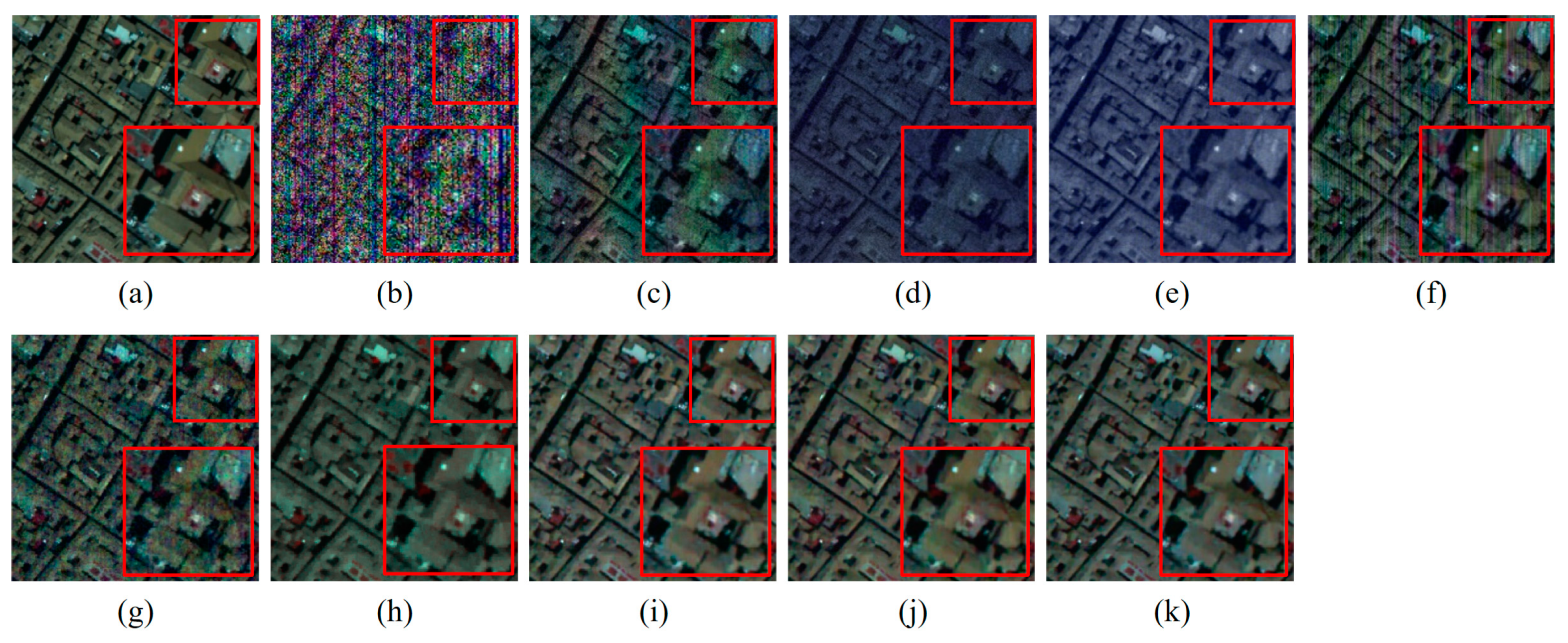
Table 1 that the performance of our method is the best except for FastHyDe. Our method significantly outperformed some typical denoising methods, such as LRMR, BM4D and NAILRMA. The FastHyDe method is a representative method for the Gaussian noise removal; it can be observed that our method achieved comparable performance in all the Gaussian noise cases compared to FastHyDe. Specifically, our MPSNR is, on average, 0.5 dB smaller than FastHyDe, but, in some metrics, such as MSSIM, our result is better than FastHyDe. For all three different Gaussian noise levels, our model achieved an improvement in MPSNR by at least 0.7 dB compared with the well-trained DL-based methods (HSID-CNN and HSI-DeNet). For visual evaluation, the false color images synthesized with band 50, 70 and 112 of the Washington DC (noise level σ = 75) were shown in Figure 5. It can be observed that our model and FastHyDe yield the closest results to the original one compared with the other methods, preserving the details while denoising.
Then, we evaluate the denoising effect of the proposed method and comparison methods in complex noise cases. The quantitative assessment results before and after denoising are shown in Table 2, and the results for visual comparison are shown in Figure 6. It can be easily seen from 
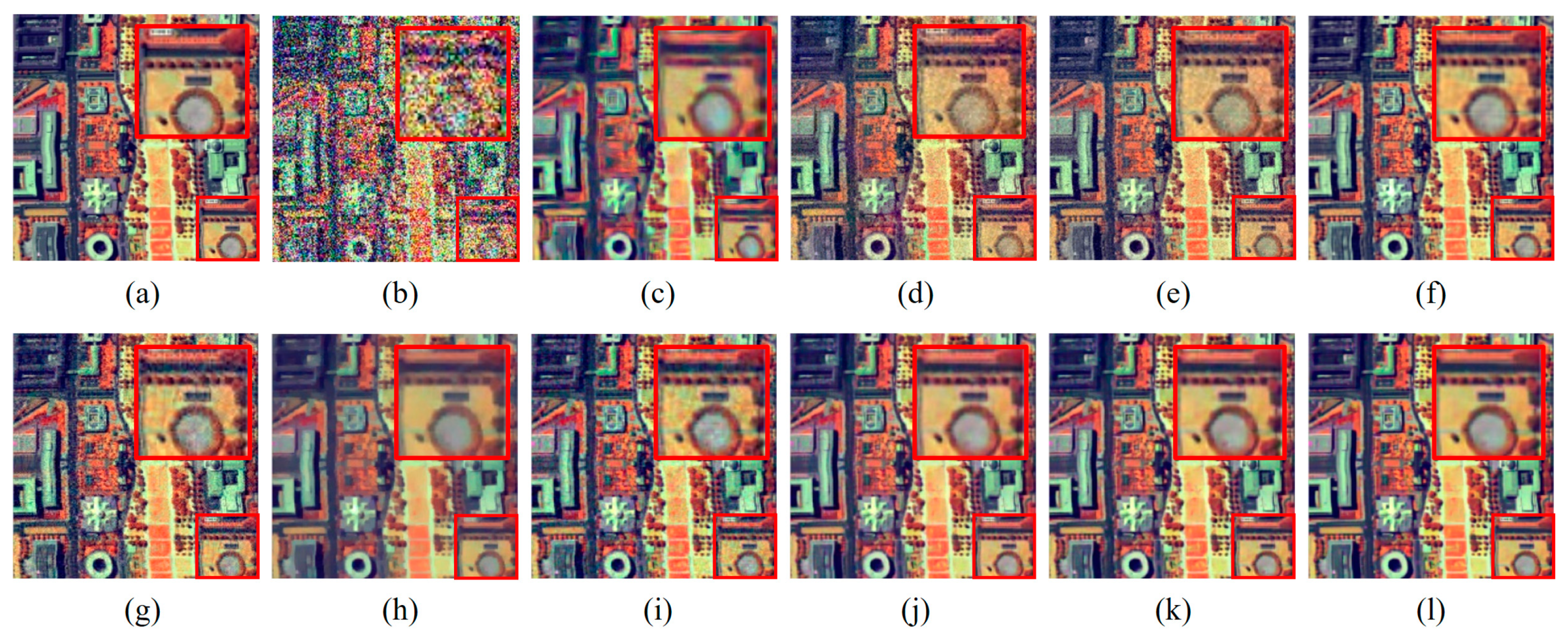
Table 2 that our method achieved better results than the other compared denoising methods in all the cases. Benefiting from the CA module and OSPA module, the former exploring the global correlation of the spectral domain, the latter reconstructing the local structures by exploring the non-local spatial correlation information, our approach yields better recovery results and higher spectral reconstruction fidelity than the other methods. The low-rank matrix-based methods, such as LRMR, NAILRMA and E3DTV, lose part of the structure information in the process of low-rank matrix approximation; therefore, the denoising effect is relatively poor, as can be seen from the denoised images in Figure 6. LRTDTV’s results are the best except for the three DL-based methods, mainly because it is based on a low-rank tensor, which fully expresses the structure of HSIs and the characteristics of noise, but it can be observed from the enlarged view in Figure 7h that there is still slight stripe noise remaining. The band-wise PSNR and SSIM are depicted in Figure 8 for further quantitative assessment; we can observe that our method obtained better PSNR and SSIM in almost all the bands compared to the other comparison methods.
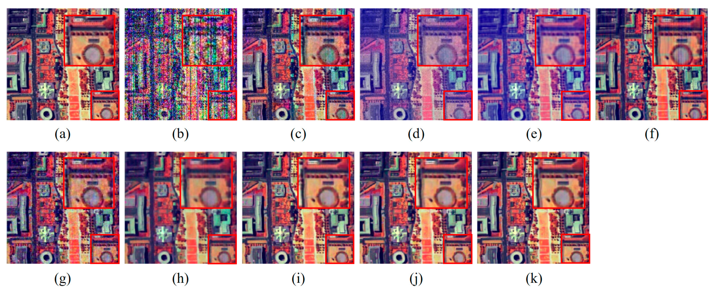
To further verify the denoising performance of the proposed model for mixed noise, we conducted synthetic noise experiments on the Pavia Center data. Noise from Case 1 to Case 5 was added to the Pavia data for testing. Table 3 shows the quantitative assessment results, and Figure 7 shows the vision comparison of the denoising results for Case 5. It can be seen that our method achieved the best results, although the gains on the Pavia data are not that large compared to those on the DC data shown in Table 2. It can be easily observed from Figure 7 that the results of our model, LRTDTV, and two DL-based methods, removing most of the mixed noise, are closest to the original reference images. The band-wise PSNR and SSIM are depicted in Figure 9; for almost all the bands in the Pavia data, our method achieves higher PSNR values and SSIM values compared to other competing methods. The experiment results on the Pavia data proved that our model has a certain generalization ability. If we need to further improve or maintain the superior performance and generalization ability of our model on different test datasets, we need to train the model on more datasets containing all these types of noise and finetune the network.

4.2. Real HSI Denoising

In this section, two real HSI data, namely Indian Pines data and GF-5 (Gaofen-5) data, were employed to further validate the effectiveness of the proposed model.
(1) Indian Pines: These data were recorded over north-western Indiana, containing 220 spectral channels, the GSD of which is 20 m. The selected scene is a size of 145 × 145 pixels, and a few bands were corrupted by heavy mixed noise (including Gaussian noise and sparse noise, e.g., impulse and stripe noise).
(2) GF-5 Data: These data were acquired by the Advanced Hyperspectral Imager (AHSI) loaded by the Chinese GF-5 satellite in January 2020 over an area of Fujian Province, China. The image wavelength range is 400 to 2500 nm, including 330 bands. Due to atmospheric absorption, 17 bands were removed, and 313 spectral bands were retained. In our experiments, an image with a size of 200 × 200 pixels was selected.
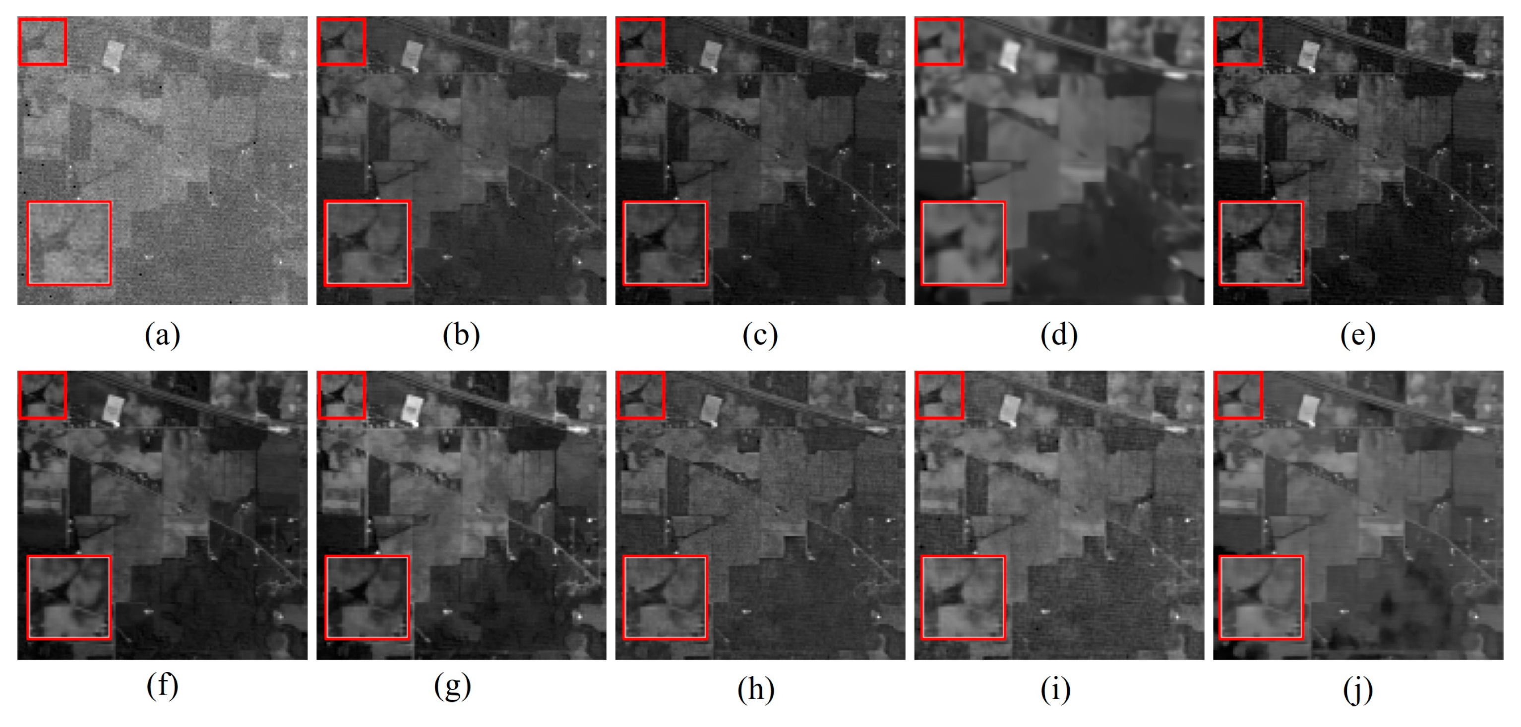
The parameters of all the traditional comparison methods were the suggested ones given in the original literature. For the DL-based methods, we used the trained network from the synthetic experiment above. To visually compare the effect of restoration, we show the second band image and the false color image synthesized with band 61, 34 and 1 in Figure 10 and Figure 11, respectively. From Figure 10, we can observe that the proposed method removed most of the noise, while other comparison methods did not completely remove complex noise. From the zoomed image of Figure 11, it can be observed that our method and LRTDTV removed most of the noise while preserving the spatial details. In addition, the corresponding computational times of all the algorithms on the Indian dataset (145 × 145 × 220) were given in Table 4. It can be seen that, although HSID-CNN and HSI-DeNet yielded less runtime, our method acquired the best result in the third shortest runtime. Considering the reason, it is mainly because matrix multiplication is used in the OSPA module of our model, which is relatively time-consuming. Nevertheless, our method is obviously much faster than all the traditional methods.
To further verify the effectiveness of denoising, a random forest (RF) classifier [65] and support vector machine (SVM) [66] were used to classify the Indian Pines data before and after denoising. Sixteen ground truth classes were employed for testing the classification accuracy. The training sets included 10% of the test samples randomly generated from each class. The overall accuracy (OA) and the kappa coefficient were given as evaluation indexes in Table 5. As can be seen, our method yields the highest classification accuracy whether using RF or SVM; the OA and kappa values corresponding to RF are 0.8812 and 0.8587, respectively, and the OA and kappa corresponding to SVM are 0.8997 and 0.8174, respectively. Figure 12 shows the results for Indian Pines using the RF classifier.
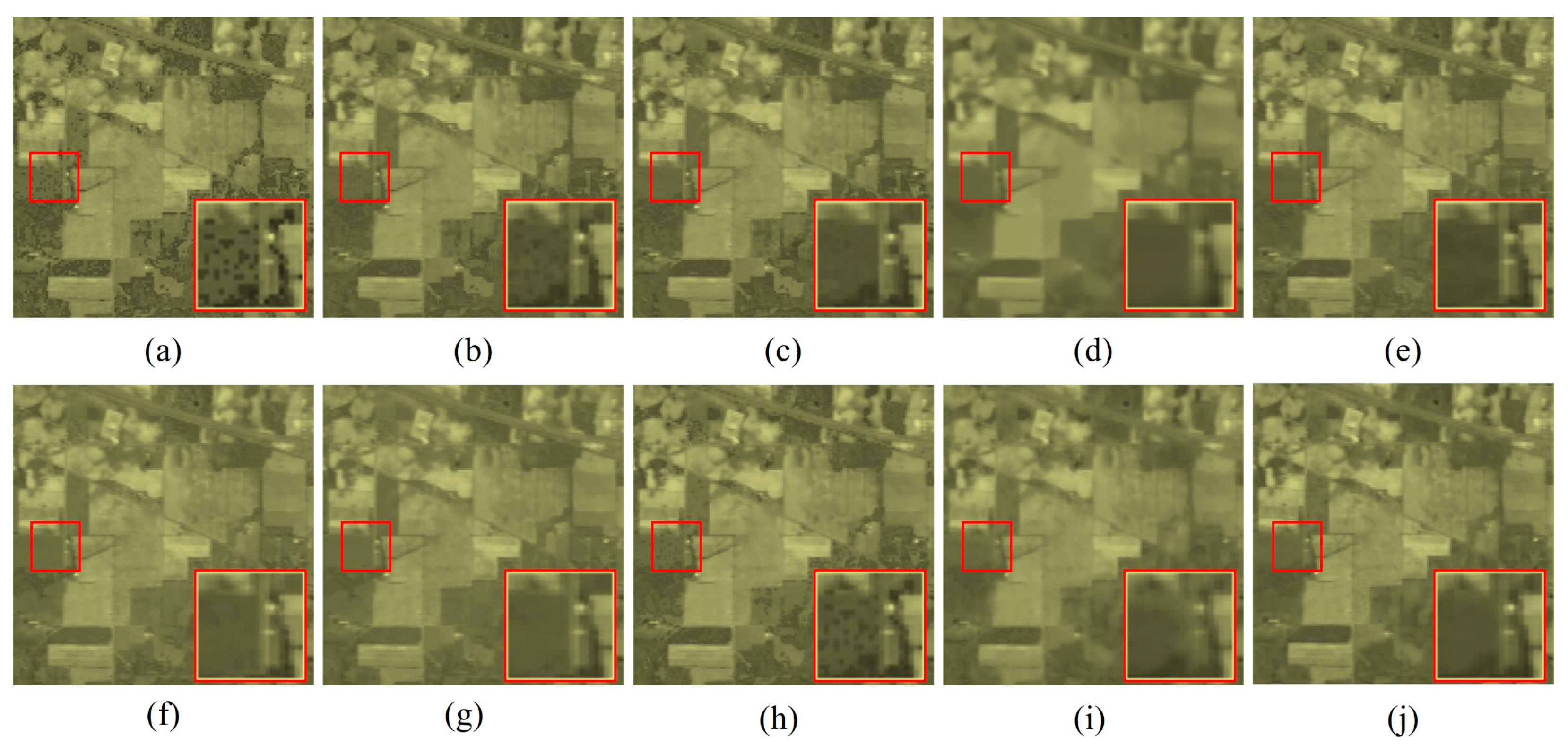
For the GF-5 data, the denoised results are shown in Figure 13 and Figure 14. Figure 14 plots second band denoised images for all the methods; it can be observed that our method exhibits the best result as most of the stripe noise was removed. Although NAILRMA also removed most of the noise and shows a relatively clean image, many structures are significantly different from the original image, probably because, in the process of low-rank matrix approximation, some structural information was removed as noise. Although the stripe noise was removed in E3DTV’s result, the image is obviously over-smoothed. LRTDTV shows a relatively better denoising effect than DL-based HSID-CNN and HSI-DeNet.
Figure 14 shows the false color images synthesized with band 1, 34 and 61 of the denoised GF-5 data. It can be observed that the proposed method achieved relatively good denoising results, and the zoomed area shows that the stripe noise and dots pattern noise were almost removed. As we mentioned above, the denoised image of NAILRMA is very clean and sharp but has obvious differences from the original image. The E3DTV result still shows over-smoothing. LRTDTV also exhibits a relatively good denoising effect, but, in the area of the blue box, there is still obvious stripe noise.

4.3. Sensitivity and Ablation Study

We examined three major determinants of our model: (a) the dimension of the orthogonal subspace, P; (b) the performance of the OSPA module; (c) the performance of the CA module.
Table 6 provides the results of the experiment on DC Mall data with different P values; a mixture noise setting in Case 5 was applied to this experiment. As we can see, when P = 30, the model was unstable and did not converge; the OSPA module cannot work effectively as a subspace projection since P is greater than the dimension size of the input. In addition to this, a lager P value also increased the difficulty of training. When P = 1, the dimension of the subspace is too small, the learning ability of the network decreased and less information would be retained, resulting in unsatisfactory training results. When P = 10 and 20, the trained model has comparable denoising performance, with MSPNRs of 33.56 and 33.45, respectively, so it can be seen that the value of P selected in our model is a robust hyperparameter within a reasonable range.
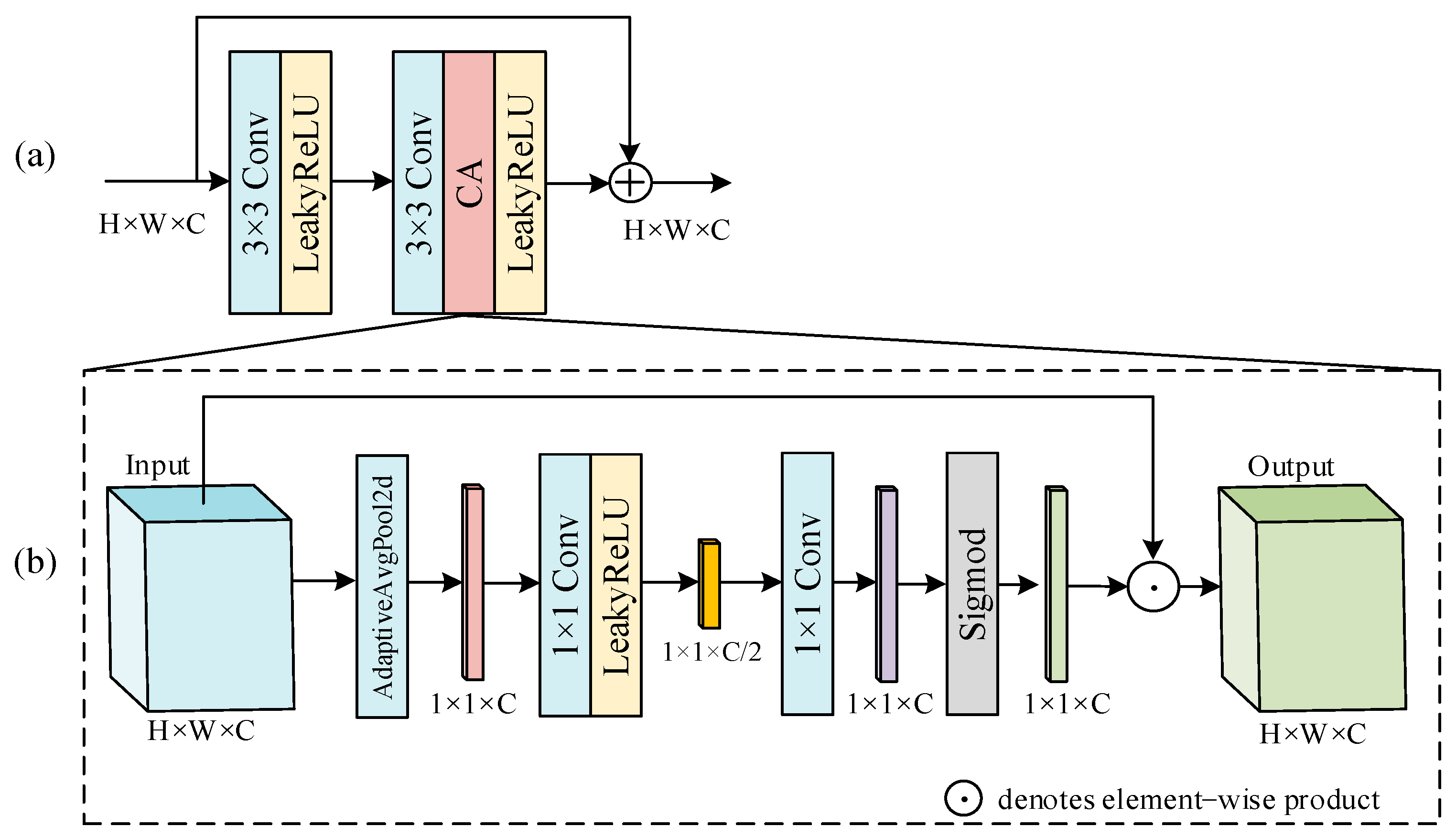
Next, to demonstrate the necessity and effectiveness of the two core modules in the proposed model, OSPA and CA, we conducted the ablation study on the effects of the OSPA and CA modules. Specifically, the ablation experiments were conducted on the Washington DC data, and the same training strategy and parameter settings as in the synthetic experiments were used. The test experiment was carried out under the condition of mixed noise (Case 5). The results are reported in Table 7.
As seen from Table 7, the original network without the OSPA and CA modules obtained the PSNR = 32.04 and SSIM = 0.8736, with slightly lower performance than HSI-DeNet. By including the OSPA modules to the model, the improvements of 0.51 and 0.0066 were achieved in MPSNR and MSSIM, respectively, while MSAM decreased by 0.0061. This is because OSPA considers the global spatial correlation, which removed spatial-related noise and recovered the original structures of images more precisely. Then, by integrating the CA modules to the model, we achieved an improvement of 0.85 and 0.0195 on MPSNR and MSSIM, respectively, and the MSAM decreased by 0.0090. This is because the CA could explore the correlations between the feature maps so that more global spectral information can be utilized. Overall, compared to the model without OSPA and CA, our original proposed model improved the MPSNR by 1.52, MSSIM by 0.0314, and decreased MSAM by 0.0135.
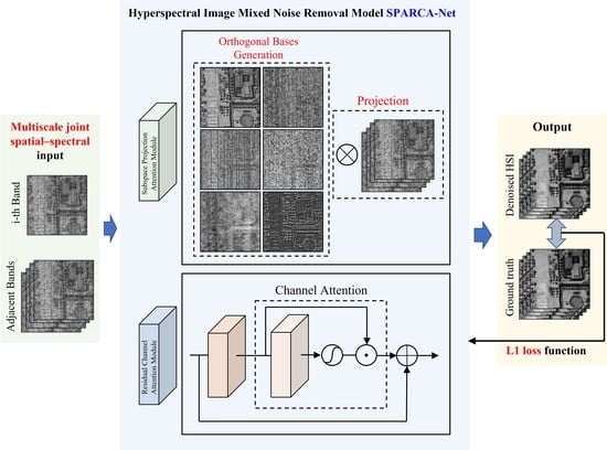
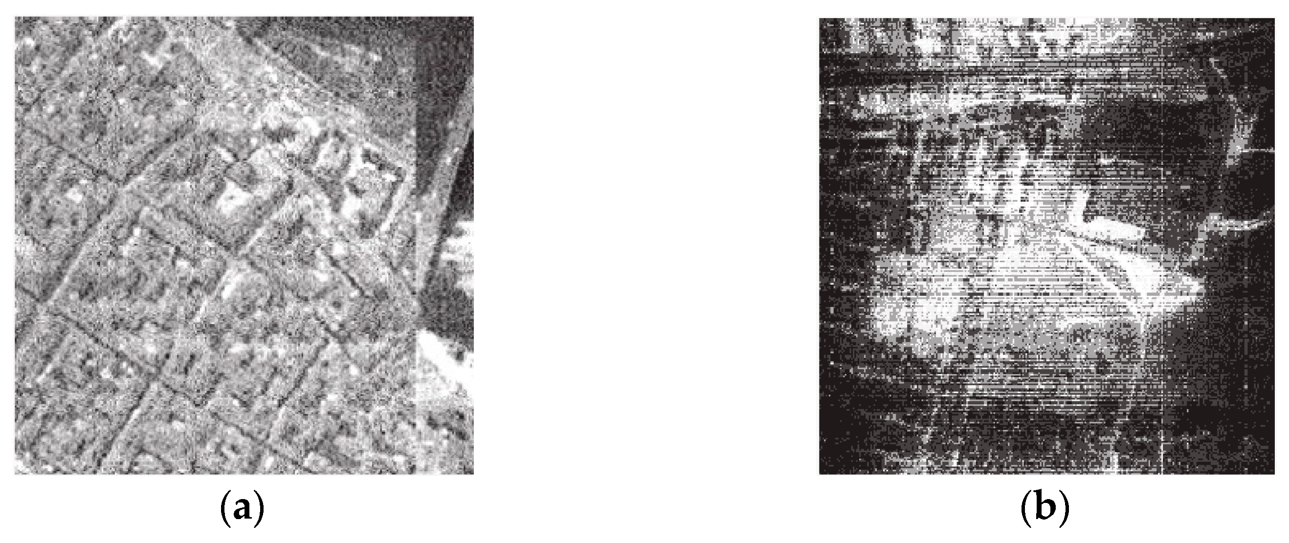
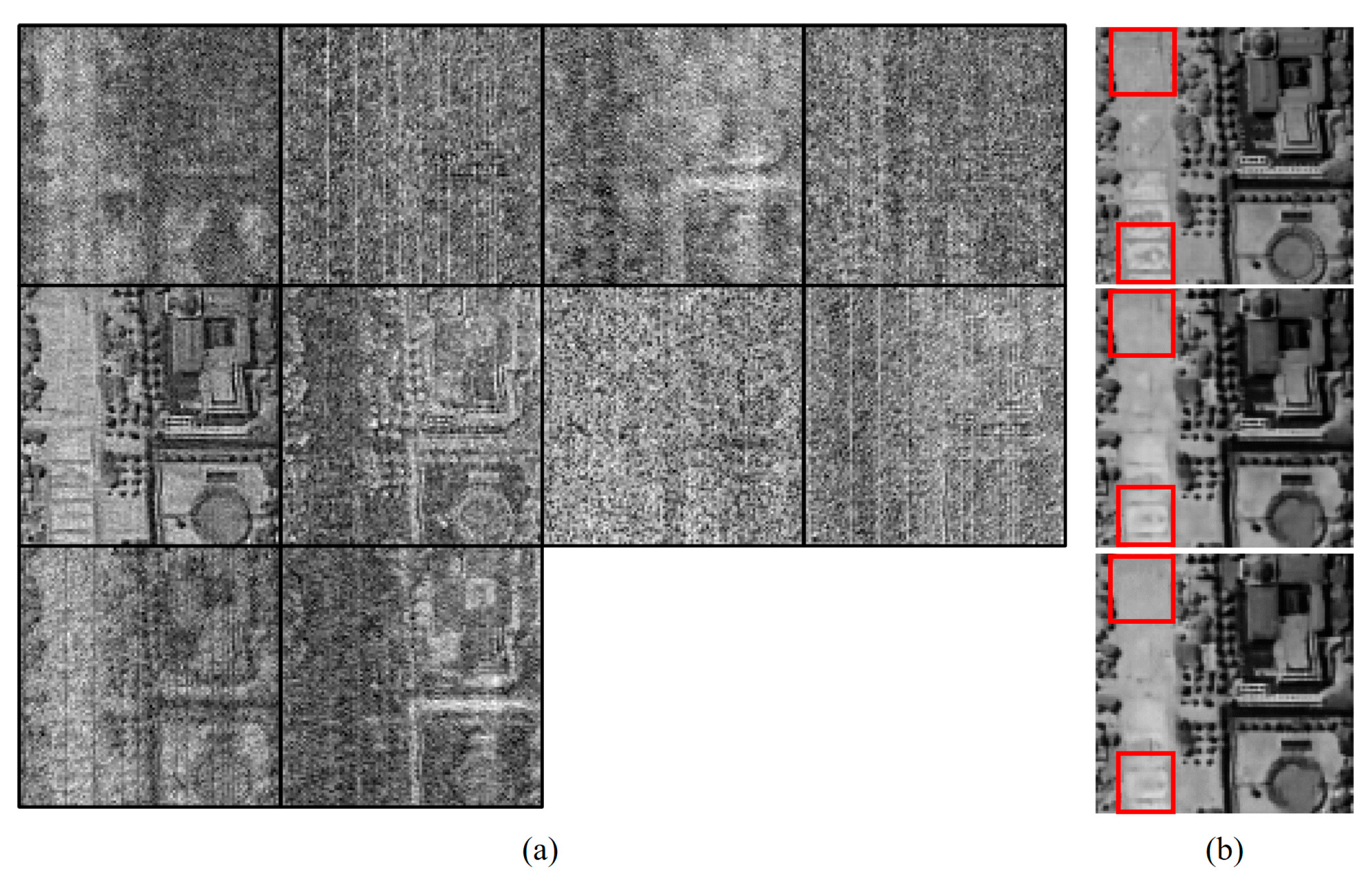
One insight of our work lies in the orthogonal subspace projection based on the spatial attention mechanism. To further understand how it works, we took the DC data as an example and examined the subspace generated by the OSPA module. We chose the experimental settings of Case 5 (complex noise) and zoomed into the lower left corner of the image for better visual observation. Figure 15a shows the visualization of the 10 basis vectors; it can be obviously seen that basically all the vectors contain the dots pattern (corresponding to Gaussian noise) that evenly spans the whole image, some vectors contain a slight stripe pattern (corresponding to stripe noise) and some vectors contain a clear spatial structure consistent with the ground truth image. Figure 15b plots band 70 of the ground truth and the denoised results with and without OSPA, respectively. We can conclude that a more detailed spatial structure is recovered in the denoised image with the virtue of OSPA.
It could be speculated that such an improvement in detailed spatial structure recovery should be attributed to the non-local and global spatial correlations explored by the OSPA module, which means that the recovered structure information can be supported by similar structures in other parts of the image. The OSPA module could effectively separate structural noise and original data by learning subspace bases and selectively remove noise through the projection process, thus yielding a restoration result with more faithful texture structure.

5. Conclusions

In this work, a novel HSI denoising network for mixed noise removal called subspace projection attention and channel attention network (SPARCA) was proposed, in which the proposed OSPA and RCA module could fully explore the local and global spatial–spectral information of the HSIs to promote a reasonable denoising effect. The proposed model takes the single band and its adjacent bands as inputs of the model, and a residual learning strategy is adopted. The RCA module is able to adaptively characterize the interdependence between channels and explore the global correlation of the spectral domain. The OSPA module could adaptively learn an orthogonal subspace projection that can be used to reconstruct the main feature maps from its subspace, which is able to facilitate spatial structure recovery by using both the local and global spatial correlations. Benefiting from this, our network could remove the mixed noise while preserving the detailed structure information. Extensive experiments conducted on two synthetic datasets and two real datasets have demonstrated the effectiveness of the proposed method and its ability to remove the mixed noise of HSIs. Moreover, an ablation study has verified the effectiveness of the proposed OSPA and CA modules.
Although the proposed network could efficiently remove mixed noise, there is still room for improvement in Gaussian noise removal compared with the traditional methods, which is also a common problem for most deep-learning-based HSI denoising methods. In the future, we may focus on further improving the model’s performance on both Gaussian noise and mixed noise removal.

Author Contributions

Conceptualization, H.S. and K.Z.; methodology, H.S.; validation, H.S. and K.Z; formal analysis, H.S.; writing—original draft preparation, H.S.; writing—review and editing, M.L. and D.Y.; visualization, C.L. and H.S.; supervision, M.L. and J.L. All authors have read and agreed to the published version of the manuscript.

Funding

This work was supported by the National Natural Science Foundation of China under Grants 61833009 and 61690212 and in part by the Heilongjiang Touyan Team. This work was partially supported by the Natural Science Foundation of Guangxi, China under Grant 2021GXNSFBA220056.

Data Availability Statement

Not applicable.

Conflicts of Interest

The authors declare no conflict of interest.

References

  1. Hong, D.; He, W.; Yokoya, N.; Yao, J.; Gao, L.; Zhang, L.; Chanussot, J.; Zhu, X. Interpretable Hyperspectral Artificial Intelligence: When Nonconvex Modeling Meets Hyperspectral Remote Sensing. IEEE Geosci. Remote Sens. Mag. 2021, 9, 52–87. [Google Scholar] [CrossRef]
  2. Zhang, B.; Sun, X.; Gao, L.; Yang, L. Endmember Extraction of Hyperspectral Remote Sensing Images Based on the Ant Colony Optimization (ACO) Algorithm. IEEE Trans. Geosci. Remote Sens. 2011, 49, 2635–2646. [Google Scholar] [CrossRef]
  3. Hong, D.; Gao, L.; Yokoya, N.; Yao, J.; Chanussot, J.; Du, Q.; Zhang, B. More Diverse Means Better: Multimodal Deep Learning Meets Remote-Sensing Imagery Classification. IEEE Trans. Geosci. Remote Sens. 2021, 59, 4340–4354. [Google Scholar] [CrossRef]
  4. Li, J.; Zheng, K.; Yao, J.; Gao, L.; Hong, D. Deep Unsupervised Blind Hyperspectral and Multispectral Data Fusion. IEEE Geosci. Remote Sens. Lett. 2022. [Google Scholar] [CrossRef]
  5. Zhang, B.; Yang, W.; Gao, L.; Chen, D. Real-Time Target Detection in Hyperspectral Images Based on Spatial-Spectral Information Extraction. EURASIP J. Adv. Signal Process. 2012, 2012, 142. [Google Scholar] [CrossRef] [Green Version]
  6. Zhang, B.; Li, S.; Jia, X.; Gao, L.; Peng, M. Adaptive Markov Random Field Approach for Classification of Hyperspectral Imagery. IEEE Geosci. Remote Sens. Lett. 2011, 8, 973–977. [Google Scholar] [CrossRef]
  7. Gao, L.; Wang, Z.; Zhuang, L.; Yu, H.; Zhang, B.; Chanussot, J. Using Low-Rank Representation of Abundance Maps and Nonnegative Tensor Factorization for Hyperspectral Nonlinear Unmixing. IEEE Trans. Geosci. Remote Sens. 2022, 60, 1–17. [Google Scholar] [CrossRef]
  8. Hong, D.; Gao, L.; Yao, J.; Zhang, B.; Plaza, A.; Chanussot, J. Graph Convolutional Networks for Hyperspectral Image Classification. IEEE Trans. Geosci. Remote Sens. 2021, 59, 5966–5978. [Google Scholar] [CrossRef]
  9. Sun, L.; Zhong, F. Mixed Noise Estimation for Hyperspectral Image Based on Multiple Bands Prediction. IEEE Geosci. Remote Sens. Lett. 2022, 19, 6007705. [Google Scholar] [CrossRef]
  10. Huang, S.; Zhang, H.; Pižurica, A. Subspace Clustering for Hyperspectral Images via Dictionary Learning with Adaptive Regularization. IEEE Trans. Geosci. Remote Sens. 2021, 60, 5524017. [Google Scholar] [CrossRef]
  11. Gao, L.; Du, Q.; Zhang, B.; Yang, W.; Wu, Y. A Comparative Study on Linear Regression-Based Noise Estimation for Hyperspectral Imagery. IEEE J. Sel. Top. Appl. Earth Obs. Remote Sens. 2013, 6, 488–498. [Google Scholar] [CrossRef] [Green Version]
  12. Zhuang, L.; Ng, M.K.; Fu, X. Hyperspectral Image Mixed Noise Removal Using Subspace Representation and Deep CNN Image Prior. Remote Sens. 2021, 13, 4098. [Google Scholar] [CrossRef]
  13. Buades, A.; Coll, B.; Morel, J.-M. A Non-Local Algorithm for Image Denoising. In Proceedings of the 2005 IEEE Computer Society Conference on Computer Vision and Pattern Recognition (CVPR’05), San Diego, CA, USA, 20–26 June 2005; Volume 2, pp. 60–65. [Google Scholar]
  14. Li, J.; Bioucas-Dias, J.M.; Plaza, A. Hyperspectral Image Segmentation Using a New Bayesian Approach with Active Learning. IEEE Trans. Geosci. Remote Sens. 2011, 49, 3947–3960. [Google Scholar] [CrossRef] [Green Version]
  15. Paris, S. A Gentle Introduction to Bilateral Filtering and Its Applications. In Proceedings of the ACM SIGGRAPH 2007 Courses, San Diego, CA, USA, 5–9 August 2007. [Google Scholar]
  16. Elad, M.; Aharon, M. Image Denoising via Sparse and Redundant Representations over Learned Dictionaries. IEEE Trans. Image Process. 2006, 15, 3736–3745. [Google Scholar] [CrossRef] [PubMed]
  17. Chang, S.G.; Yu, B.; Vetterli, M. Adaptive Wavelet Thresholding for Image Denoising and Compression. IEEE Trans. Image Process. 2000, 9, 1532–1546. [Google Scholar] [CrossRef] [Green Version]
  18. Dabov, K.; Foi, A.; Katkovnik, V.; Egiazarian, K. Image Denoising by Sparse 3-D Transform-Domain Collaborative Filtering. IEEE Trans. Image Process. 2007, 16, 2080–2095. [Google Scholar] [CrossRef]
  19. Maggioni, M.; Katkovnik, V.; Egiazarian, K.; Foi, A. Nonlocal Transform-Domain Filter for Volumetric Data Denoising and Reconstruction. IEEE Trans. Image Process. 2013, 22, 119–133. [Google Scholar] [CrossRef]
  20. Green, A.A.; Berman, M.; Switzer, P.; Craig, M.D. A Transformation for Ordering Multispectral Data in Terms of Image Quality with Implications for Noise Removal. IEEE Trans. Geosci. Remote Sens. 1988, 26, 65–74. [Google Scholar] [CrossRef] [Green Version]
  21. Donoho, D.L.; Johnstone, I.M. Adapting to Unknown Smoothness via Wavelet Shrinkage. J. Am. Stat. Assoc. 1995, 90, 1200–1224. [Google Scholar] [CrossRef]
  22. Chang, C.-I.; Du, Q. Interference and Noise-Adjusted Principal Components Analysis. IEEE Trans. Geosci. Remote Sens. 1999, 37, 2387–2396. [Google Scholar] [CrossRef] [Green Version]
  23. Renard, N.; Bourennane, S.; Blanc-Talon, J. Denoising and Dimensionality Reduction Using Multilinear Tools for Hyperspectral Images. IEEE Geosci. Remote Sens. Lett. 2008, 5, 138–142. [Google Scholar] [CrossRef]
  24. Fan, H.; Chen, Y.; Guo, Y.; Zhang, H.; Kuang, G. Hyperspectral Image Restoration Using Low-Rank Tensor Recovery. IEEE J. Sel. Top. Appl. Earth Obs. Remote Sens. 2017, 10, 4589–4604. [Google Scholar] [CrossRef]
  25. Zhang, H.; He, W.; Zhang, L.; Shen, H.; Yuan, Q. Hyperspectral Image Restoration Using Low-Rank Matrix Recovery. IEEE Trans. Geosci. Remote Sens. 2014, 52, 4729–4743. [Google Scholar] [CrossRef]
  26. He, W.; Zhang, H.; Zhang, L.; Shen, H. Hyperspectral Image Denoising via Noise-Adjusted Iterative Low-Rank Matrix Approximation. IEEE J. Sel. Top. Appl. Earth Obs. Remote Sens. 2015, 8, 3050–3061. [Google Scholar] [CrossRef]
  27. Fan, H.; Li, J.; Yuan, Q.; Liu, X.; Ng, M. Hyperspectral Image Denoising with Bilinear Low Rank Matrix Factorization. Signal Processing 2019, 163, 132–152. [Google Scholar] [CrossRef]
  28. Xue, J.; Zhao, Y.; Liao, W.; Chan, J.C.-W. Nonlocal Low-Rank Regularized Tensor Decomposition for Hyperspectral Image Denoising. IEEE Trans. Geosci. Remote Sens. 2019, 57, 5174–5189. [Google Scholar] [CrossRef]
  29. Yuan, Q.; Zhang, L.; Shen, H. Hyperspectral Image Denoising Employing a Spectral–Spatial Adaptive Total Variation Model. IEEE Trans. Geosci. Remote Sens. 2012, 50, 3660–3677. [Google Scholar] [CrossRef]
  30. Aggarwal, H.K.; Majumdar, A. Hyperspectral Image Denoising Using Spatio-Spectral Total Variation. IEEE Geosci. Remote Sens. Lett. 2016, 13, 442–446. [Google Scholar] [CrossRef]
  31. Peng, J.; Xie, Q.; Zhao, Q.; Wang, Y.; Meng, D. Enhanced 3DTV Regularization and Its Applications on Hyper-Spectral Image Denoising and Compressed Sensing. arXiv 2018, arXiv:1809.06591. [Google Scholar]
  32. Gao, L.; Yao, D.; Li, Q.; Zhuang, L.; Zhang, B.; Bioucas-Dias, J.M. A New Low-Rank Representation Based Hyperspectral Image Denoising Method for Mineral Mapping. Remote Sens. 2017, 9, 1145. [Google Scholar] [CrossRef] [Green Version]
  33. He, W.; Zhang, H.; Zhang, L.; Shen, H. Total-Variation-Regularized Low-Rank Matrix Factorization for Hyperspectral Image Restoration. IEEE Trans. Geosci. Remote Sens. 2016, 54, 178–188. [Google Scholar] [CrossRef]
  34. He, W.; Zhang, H.; Shen, H.; Zhang, L. Hyperspectral Image Denoising Using Local Low-Rank Matrix Recovery and Global Spatial–Spectral Total Variation. IEEE J. Sel. Top. Appl. Earth Obs. Remote Sens. 2018, 11, 713–729. [Google Scholar] [CrossRef]
  35. Wang, Y.; Peng, J.; Zhao, Q.; Leung, Y.; Zhao, X.-L.; Meng, D. Hyperspectral Image Restoration Via Total Variation Regularized Low-Rank Tensor Decomposition. IEEE J. Sel. Top. Appl. Earth Obs. Remote Sens. 2018, 11, 1227–1243. [Google Scholar] [CrossRef] [Green Version]
  36. Zhuang, L.; Bioucas-Dias, J.M. Fast Hyperspectral Image Denoising and Inpainting Based on Low-Rank and Sparse Representations. IEEE J. Sel. Top. Appl. Earth Obs. Remote Sens. 2018, 11, 730–742. [Google Scholar] [CrossRef]
  37. He, W.; Yao, Q.; Li, C.; Yokoya, N.; Zhao, Q. Non-Local Meets Global: An Integrated Paradigm for Hyperspectral Denoising. In Proceedings of the IEEE/CVF Conference on Computer Vision and Pattern Recognition, Long Beach, CA, USA, 15–20 June 2019; pp. 6868–6877. [Google Scholar]
  38. Zhuang, L.; Ng, M.K. Hyperspectral Mixed Noise Removal by L1-Norm-Based Subspace Representation. IEEE J. Sel. Top. Appl. Earth Obs. Remote Sens. 2020, 13, 1143–1157. [Google Scholar] [CrossRef]
  39. Shi, Q.; Tang, X.; Yang, T.; Liu, R.; Zhang, L. Hyperspectral Image Denoising Using a 3-D Attention Denoising Network. IEEE Trans. Geosci. Remote Sens. 2021, 59, 10348–10363. [Google Scholar] [CrossRef]
  40. Zhang, K.; Zuo, W.; Chen, Y.; Meng, D.; Zhang, L. Beyond a Gaussian Denoiser: Residual Learning of Deep CNN for Image Denoising. IEEE Trans. Image Process. 2017, 26, 3142–3155. [Google Scholar] [CrossRef] [Green Version]
  41. Gao, L.; Han, Z.; Hong, D.; Zhang, B.; Chanussot, J. CyCU-Net: Cycle-Consistency Unmixing Network by Learning Cascaded Autoencoders. IEEE Trans. Geosci. Remote Sens. 2022, 60, 5503914. [Google Scholar] [CrossRef]
  42. Hong, D.; Han, Z.; Yao, J.; Gao, L.; Zhang, B.; Plaza, A.; Chanussot, J. SpectralFormer: Rethinking Hyperspectral Image Classification with Transformers. IEEE Trans. Geosci. Remote Sens. 2021, 60, 5518615. [Google Scholar] [CrossRef]
  43. Hong, D.; Yao, J.; Meng, D.; Xu, Z.; Chanussot, J. Multimodal GANs: Toward Crossmodal Hyperspectral–Multispectral Image Segmentation. IEEE Trans. Geosci. Remote Sens. 2021, 59, 5103–5113. [Google Scholar] [CrossRef]
  44. Zheng, K.; Gao, L.; Hong, D.; Zhang, B.; Chanussot, J. NonRegSRNet: A Non-Rigid Registration Hyperspectral Super-Resolution Network. IEEE Trans. Geosci. Remote Sens. 2021, 60, 1–16. [Google Scholar] [CrossRef]
  45. Yao, J.; Meng, D.; Zhao, Q.; Cao, W.; Xu, Z. Nonconvex-Sparsity and Nonlocal-Smoothness Based Blind Hyperspectral Unmixing. IEEE Trans. Image Process. 2019, 28, 2991–3006. [Google Scholar] [CrossRef] [PubMed]
  46. Yao, J.; Hong, D.; Xu, L.; Meng, D.; Chanussot, J.; Xu, Z. Sparsity-Enhanced Convolutional Decomposition: A Novel Tensor-Based Paradigm for Blind Hyperspectral Unmixing. IEEE Trans. Geosci. Remote Sens. 2022, 60, 5505014. [Google Scholar] [CrossRef]
  47. Hong, D.; Yokoya, N.; Chanussot, J.; Zhu, X.X. An Augmented Linear Mixing Model to Address Spectral Variability for Hyperspectral Unmixing. IEEE Trans. Image Process. 2019, 28, 1923–1938. [Google Scholar] [CrossRef] [PubMed] [Green Version]
  48. Chang, Y.; Yan, L.; Fang, H.; Zhong, S.; Liao, W. HSI-DeNet: Hyperspectral Image Restoration via Convolutional Neural Network. IEEE Trans. Geosci. Remote Sens. 2019, 57, 667–682. [Google Scholar] [CrossRef]
  49. Yuan, Q.; Zhang, Q.; Li, J.; Shen, H.; Zhang, L. Hyperspectral Image Denoising Employing a Spatial–Spectral Deep Residual Convolutional Neural Network. IEEE Trans. Geosci. Remote Sens. 2019, 57, 1205–1218. [Google Scholar] [CrossRef] [Green Version]
  50. Zhang, Q.; Yuan, Q.; Li, J.; Liu, X.; Shen, H.; Zhang, L. Hybrid Noise Removal in Hyperspectral Imagery With a Spatial–Spectral Gradient Network. IEEE Trans. Geosci. Remote Sens. 2019, 57, 7317–7329. [Google Scholar] [CrossRef]
  51. Wang, Z.; Shao, Z.; Huang, X.; Wang, J.; Lu, T. SSCAN: A Spatial–Spectral Cross Attention Network for Hyperspectral Image Denoising. IEEE Geosci. Remote Sens. Lett. 2022, 19, 5508805. [Google Scholar] [CrossRef]
  52. Cao, X.; Fu, X.; Xu, C.; Meng, D. Deep Spatial-Spectral Global Reasoning Network for Hyperspectral Image Denoising. IEEE Trans. Geosci. Remote Sens. 2022, 60, 5504714. [Google Scholar] [CrossRef]
  53. Cheng, Y.; Zhang, K.; Xu, Z. Theory of Matrix, 3rd ed.; Northwestern Polytechnic University Press: Xi’an, China, 2006. [Google Scholar]
  54. Hu, J.; Shen, L.; Sun, G. Squeeze-and-Excitation Networks. In Proceedings of the IEEE Conference on Computer Vision and Pattern Recognition, Salt Lake City, UT, USA, 18–62 June 2018; pp. 7132–7141. [Google Scholar]
  55. Dai, T.; Cai, J.; Zhang, Y.; Xia, S.-T.; Zhang, L. Second-Order Attention Network for Single Image Super-Resolution. In Proceedings of the IEEE/CVF Conference on Computer Vision and Pattern Recognition, Long Beach, CA, USA, 15–20 June 2019; pp. 11065–11074. [Google Scholar]
  56. Qin, Z.; Zhang, P.; Wu, F.; Li, X. Fcanet: Frequency Channel Attention Networks. In Proceedings of the IEEE/CVF International Conference on Computer Vision, Montreal, BC, Canada, 11–17 October 2021; pp. 783–792. [Google Scholar]
  57. Hu, H.; Gu, J.; Zhang, Z.; Dai, J.; Wei, Y. Relation Networks for Object Detection. In Proceedings of the IEEE Conference on Computer Vision and Pattern Recognition, Salt Lake City, UT, USA, 18–62 June 2018; pp. 3588–3597. [Google Scholar]
  58. Chen, Y.; Rohrbach, M.; Yan, Z.; Shuicheng, Y.; Feng, J.; Kalantidis, Y. Graph-Based Global Reasoning Networks. In Proceedings of the IEEE/CVF Conference on Computer Vision and Pattern Recognition, Long Beach, CA, USA, 15–20 June 2019; pp. 433–442. [Google Scholar]
  59. Liu, M.; Wang, Z.; Ji, S. Non-Local Graph Neural Networks. IEEE Trans. Pattern Anal. Mach. Intell. 2021. [Google Scholar] [CrossRef]
  60. Yao, J.; Hong, D.; Chanussot, J.; Meng, D.; Zhu, X.; Xu, Z. Cross-Attention in Coupled Unmixing Nets for Unsupervised Hyperspectral Super-Resolution. In Proceedings of the 16th European Conference on Computer Vision (ECCV), Glasgow, UK, 23–28 August 2020; pp. 208–224. [Google Scholar]
  61. Meyer, C.D. Matrix Analysis and Applied Linear Algebra; Siam: Philadelphia, PA, USA, 2000; Volume 71. [Google Scholar]
  62. Zhang, Y.; Li, K.; Li, K.; Wang, L.; Zhong, B.; Fu, Y. Image Super-Resolution Using Very Deep Residual Channel Attention Networks. In Proceedings of the European Conference on Computer Vision (ECCV), Munich, Germany, 14–24 May 2018; pp. 286–301. [Google Scholar]
  63. Paszke, A.; Gross, S.; Massa, F.; Lerer, A.; Bradbury, J.; Chanan, G.; Killeen, T.; Lin, Z.M.; Gimelshein, N.; Antiga, L.; et al. PyTorch: An Imperative Style, High-Performance Deep Learning Library. In Proceedings of the 33rd Conference on Neural Information Processing Systems (NeurIPS), Vancouver, BC, Canada, 8–14 December 2019. [Google Scholar]
  64. Kingma, D.P.; Ba, J. Adam: A Method for Stochastic Optimization. arXiv 2014, arXiv:1412.6980. [Google Scholar]
  65. Breiman, L. Random Forests. Mach. Learn. 2001, 45, 5–32. [Google Scholar] [CrossRef] [Green Version]
  66. Melgani, F.; Bruzzone, L. Classification of hyperspectral remote sensing images with support vector machines. IEEE Trans. Geosci. Remote Sens. 2004, 42, 1778–1790. [Google Scholar] [CrossRef] [Green Version]
Figure 1. Observed HSIs contaminated by mixed noise. (a) The second band image of Pavia University dataset; (b) the 139th band image of URBAN dataset.
Remotesensing 14 02071 g001
Figure 2. Flowchart showing the details of the proposed SPARCA-Net model for HSI denoising.
Remotesensing 14 02071 g002
Figure 3. Details of the orthogonal subspace projection attention (OSPA) module.
Remotesensing 14 02071 g003
Figure 4. The illustration of the RCA. (a) Details of RCA module; (b) details of CA sub-module.
Remotesensing 14 02071 g004
Figure 5. False color images synthesized with band 50, 70 and 112 of denoised Washington DC data in Gaussian noise case; σ = 75 . (a) Clean; (b) noisy; (c) BM4D; (d) LRMR; (e) NAILRMA; (f) FastHyDe; (g) L1HyMixDe; (h) E3DTV; (i) LRTDTV; (j) HSI-DeNet; (k) HSID-CNN; (l) ours.
Remotesensing 14 02071 g005
Figure 6. False color images synthesized with band 50, 70 and 110 of the denoised Washington DC data in mixture noise case. (a) Clean; (b) noisy; (c) LRMR; (d) NAILRMA; (e) NGmeet; (f) L1HyMixDe; (g) E3DTV; (h) LRTDTV; (i) HSI-DeNet; (j) HSID-CNN; (k) ours.
Remotesensing 14 02071 g006
Figure 7. False color images synthesized with band 14, 24 and 54 of the denoised Pavia Center data in mixture noise case. (a) Clean; (b) noisy; (c) LRMR; (d) NAILRMA; (e) NGmeet; (f) L1HyMixDe; (g) E3DTV; (h) LRTDTV; (i) HSI-DeNet; (j) HSID-CNN; (k) ours.
Remotesensing 14 02071 g007
Figure 8. Band-wise PSNR values in the first row and band-wise SSIM values in the second row for denoised Washington DC data. Subfigures in (a,f), (b,g), (c,h), (d,i) and (e,j) correspond to Case 1, Case 2, Case 3, Case 4 and Case 5, respectively.
Remotesensing 14 02071 g008
Figure 9. Band-wise PSNR values in the first row and band-wise SSIM values in the second row for denoised Pavia Center data. Subfigures in (a,f), (b,g), (c,h), (d,i) and (e,j) correspond to Case 1, Case 2, Case 3, Case 4 and Case 5, respectively.
Remotesensing 14 02071 g009
Figure 10. The denoised results on band 2 of the Indian Pines data. (a) Original; (b) LRMR; (c) NAILRMA; (d) NGmeet; (e) L1HyMixDe; (f) E3DTV; (g) LRTDTV; (h) HSI-DeNet; (i) HSID-CNN; (j) ours.
Remotesensing 14 02071 g010
Figure 11. False color images synthesized with band 61, 34 and 1 of denoised Indian Pines data. (a) Original; (b) LRMR; (c) NAILRMA; (d) NGmeet; (e) L1HyMixDe; (f) E3DTV; (g) LRTDTV; (h) HSI-DeNet; (i) HSID-CNN; (j) ours.
Remotesensing 14 02071 g011
Figure 12. Classification results for Indian Pines. (a) Original; (b) LRMR; (c) NAILRMA; (d) NGmeet; (e) L1HyMixDe; (f) E3DTV; (g) LRTDTV; (h) HSI-DeNet; (i) HSID-CNN; (j) ours; (k) ground truth and class labels.
Remotesensing 14 02071 g012
Figure 13. The denoised results on band 2 of the GF-5 data. (a) Original; (b) LRMR; (c) NAILRMA; (d) NGmeet; (e) L1HyMixDe; (f) E3DTV; (g) LRTDTV; (h) HSI-DeNet; (i) HSID-CNN; (j) ours.
Remotesensing 14 02071 g013
Figure 14. False color images synthesized with band 1, 34 and 61 of the denoised GF-5 data. (a) Original; (b) LRMR; (c) NAILRMA; (d) NGmeet; (e) L1HyMixDe; (f) E3DTV; (g) LRTDTV; (h) HSI-DeNet; (i) HSID-CNN; (j) ours.
Remotesensing 14 02071 g014
Figure 15. Base visualization. (a) Visualization of basis vectors; (b) ground truth (up), denoising result with OSPA (middle) and result without OSPA (down).
Remotesensing 14 02071 g015
Table 1. Quantitative assessment of different algorithms applied to Washington DC Mall data with Gaussian i.i.d. noise.
IndexNoisy HSIBM4DLRMRNAILRMAFastHyDeL1HyMixDeE3DTVLRTDTVHSI-DeNetHSID-CNNOurs
σ = 25
MPSNR20.1733.0234.6937.1638.8436.6034.2335.8137.5037.4638.31
MSSIM0.35600.89520.91750.94370.96290.93430.92840.94410.96080.95880.9652
MSAM0.33830.07380.06080.04450.03570.04740.10580.05190.04460.04540.0403
σ = 50
MPSNR14.1529.4529.9032.4635.1031.5730.8933.3633.6033.4234.46
MSSIM0.14980.78880.80350.86550.92540.83620.85940.89970.90650.90390.9206
MSAM0.60800.11160.10450.07490.05360.08210.13260.07210.07020.07190.0614
σ = 75
MPSNR10.6327.4527.0529.7232.9328.9029.4830.9631.3731.6932.44
MSSIM0.07800.69560.69450.79590.89290.75860.82410.83170.85580.86120.8790
MSAM0.80220.14090.14400.10150.06790.10830.15960.09790.08930.08620.0775
Table 2. Quantitative assessment of different algorithms applied to Washington DC Mall data with mixture noise cases.
IndexNoisy HSILRMR NAILRMANGmeetL1HyMixDeE3DTVLRTDTVHSI-DeNetHSID-CNNOurs
Case 1 (Gaussian noise)
MPSNR14.5430.3032.2932.5931.3132.0433.1134.0833.8734.74
MSSIM0.17250.81030.86840.87610.90290.85590.90630.91430.91080.9253
MSAM0.62610.10250.07660.10270.06200.08920.07460.06610.06790.0601
Case 2 (Gaussian noise + Stripes)
MPSNR14.4530.6232.1132.4831.0031.8933.0533.1633.4234.45
MSSIM0.16970.82960.86650.87440.89720. 85240.90550.89700.90360.9211
MSAM0.62910.09700.07850.10330.06490. 09090.07840.07540.07170.0628
Case 3 (Gaussian noise + Deadlines)
MPSNR14.3629.1931.1131.4929.0031.0032.3134.0133.2234.39
MSSIM0.16470.79260.83530.86890.85470.84340.89830.91430.90030.9213
MSAM0.64310.12480.09440.11660.09270.10420.08690.06660.07420.0629
Case 4 (Gaussian noise + Impulse noise)
MPSNR12.6928.7026.6228.8029.4431.0331.6933.0532.5233.93
MSSIM0.12560.75850.74230.82040.87870.83760.88150.89330.88530.9118
MSAM0.73440.15710.28620.28250.08800.10920.12360.07550.07900.0668
Case 5 (Mixture noise)
MPSNR12.3827.1125.0726.7126.4129.4430.2232.4731.8333.56
MSSIM0.11630.72530.71160.79230.80600.80650.85850.88040.86830.9050
MSAM0.76340.18670.31750.31080.14170.13360.13370.07990.08540.0697
Table 3. Quantitative assessment of different algorithms applied to Pavia Centre data with mixture noise cases.
IndexNoisy HSILRMR NAILRMANGmeetL1HyMixDeE3DTVLRTDTVHSI-DeNetHSID-CNNOurs
Case 1 (Gaussian noise)
MPSNR14.4527.5930.7029.2231.5328.6331.9831.3731.5631.98
MSSIM0.16360.74130.86290.79620.87390.76780.87600.89560.90170.9099
MSAM0.91540.32230.15590.37120.14830.27140.17600.17190.14880.1342
Case 2 (Gaussian noise + Stripes)
MPSNR14.3928.7330.5829.0631.2428.4231.1131.2131.4231.70
MSSIM0.16190.79370.86100.79190.86600.76110.85880.89640.89630.9070
MSAM0.91860.25790.15900.37940.16010.27710.15450.16560.15430.1333
Case 3 (Gaussian noise + Deadlines)
MPSNR14.4728.1230.1929.0529.3728.0430.4431.2931.3931.72
MSSIM0.16070.78440.85910.80220.81570.75170.85070.89490.89520.9073
MSAM0.92700.28320.17350.37120.24630.29540.14560.16450.14950.1323
Case 4 (Gaussian noise + Impulse noise)
MPSNR12.9126.8924.8525.2729.7927.9530.3130.5730.6830.83
MSSIM0.13230.72030.70070.72260.82670.72760.83490.88060.87660.8902
MSAM0.91740.43540.37360.49670.18430.30980.16270.16600.17350.1419
Case 5 (Mixture noise)
MPSNR12.7225.7123.8024.3127.7527.0129.0530.1929.7930.35
MSSIM0.12460.69330.66940.70250.76550.70380.82090.87420.86160.8777
MSAM0.93130.46010.39850.50470.27640.34200.29120.17870.18440.1654
Table 4. Average runtime comparisons for HSI denoising methods on Indian Pines (145 × 145 × 220).
MethodLRMR NAILRMANGmeetL1HyMixDeE3DTVLRTDTVHSI-DeNetHSID-CNNOurs
Time (s)127.8116.533.937.444.4170.16.13.317.0
Table 5. Classification accuracy results for Indian Pines.
IndexOriginalLRMRNAILRMANGmeetL1HyMixDeE3DTVLRTDTVHSI-DeNetHSID-CNNOurs
RF
OA0.80650.85100.85200.85640.83700.86390.80680.85430.84140.8812
Kappa0.70710.81500.81110.81340.76130.79210.73530.77010.78370.8587
SVM
OA0.76060.82100.79260.59480.80080.79210.59120.86650.88620.8997
Kappa0.68410.78000.75920.56610.77720.74570.56500.78570.81580.8174
Table 6. Effect of orthogonal subspace dimension P on Washington DC data with mixture noise.
P1102030
MPSNR33.0433.5633.45-
MSSIM0.89520.90500.9026-
MSAM0.07420.06970.0710-
Table 7. Results of the ablation study on the effect of OSPA and CA modules.
Component ModulesAccuracy Indicators
OSPACAMPSNRMSSIMMSAM
32.040.87360.0832
32.550.88650.0771
32.890.89310.0742
33.560.90500.0697
Publisher’s Note: MDPI stays neutral with regard to jurisdictional claims in published maps and institutional affiliations.

