
How Much of a Pixel Needs to Burn to Be Detected by Satellites? A Spectral Modeling Experiment Based on Ecosystem Data from Yellowstone National Park, USA


Abstract
:
1. Introduction
2. Materials and Methods
2.1. Study Area
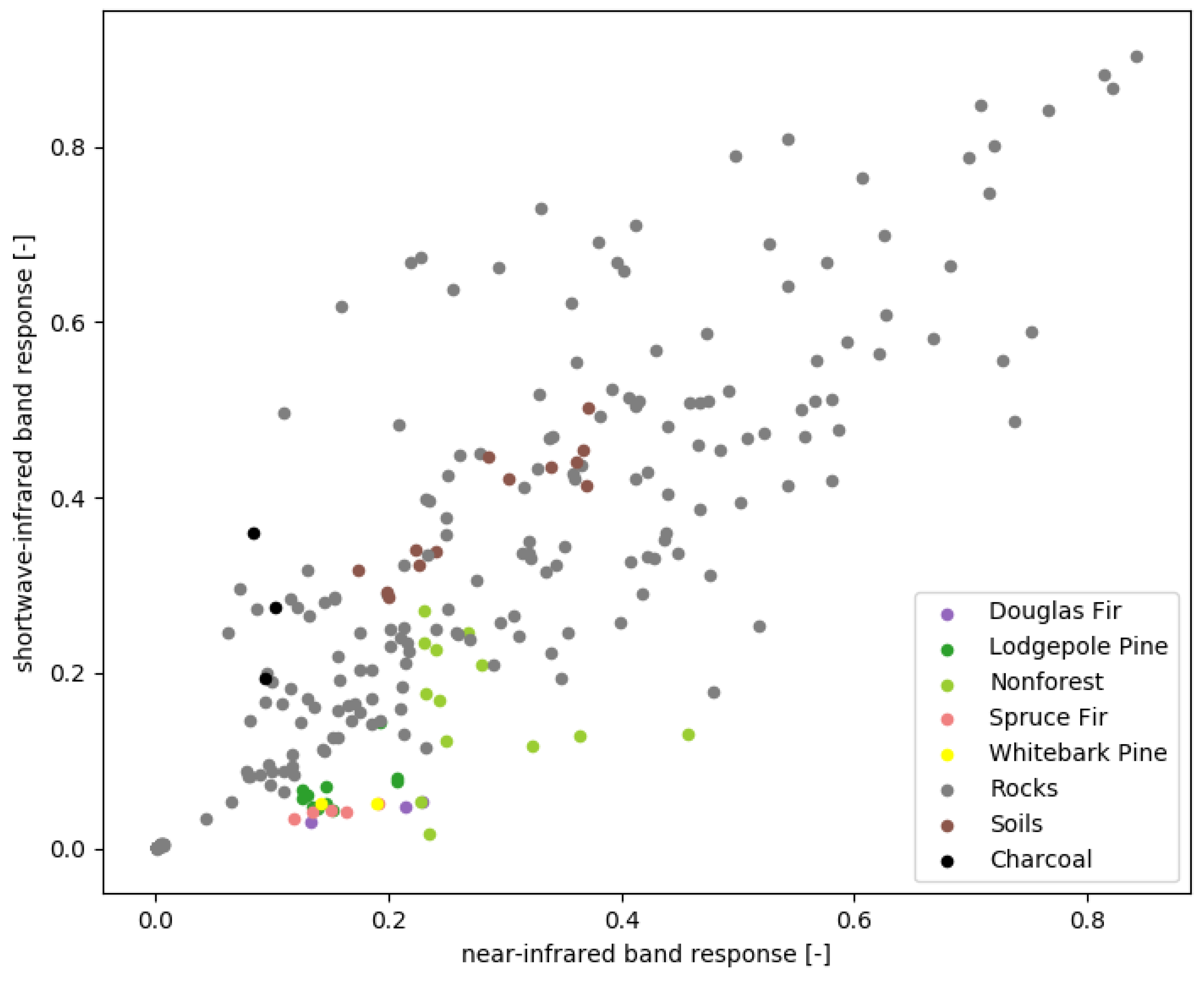
2.2. Endmember Selection
2.3. Sample Preparation
2.4. Modeling Burned Area Response
2.5. Data Aggregation
3. Results
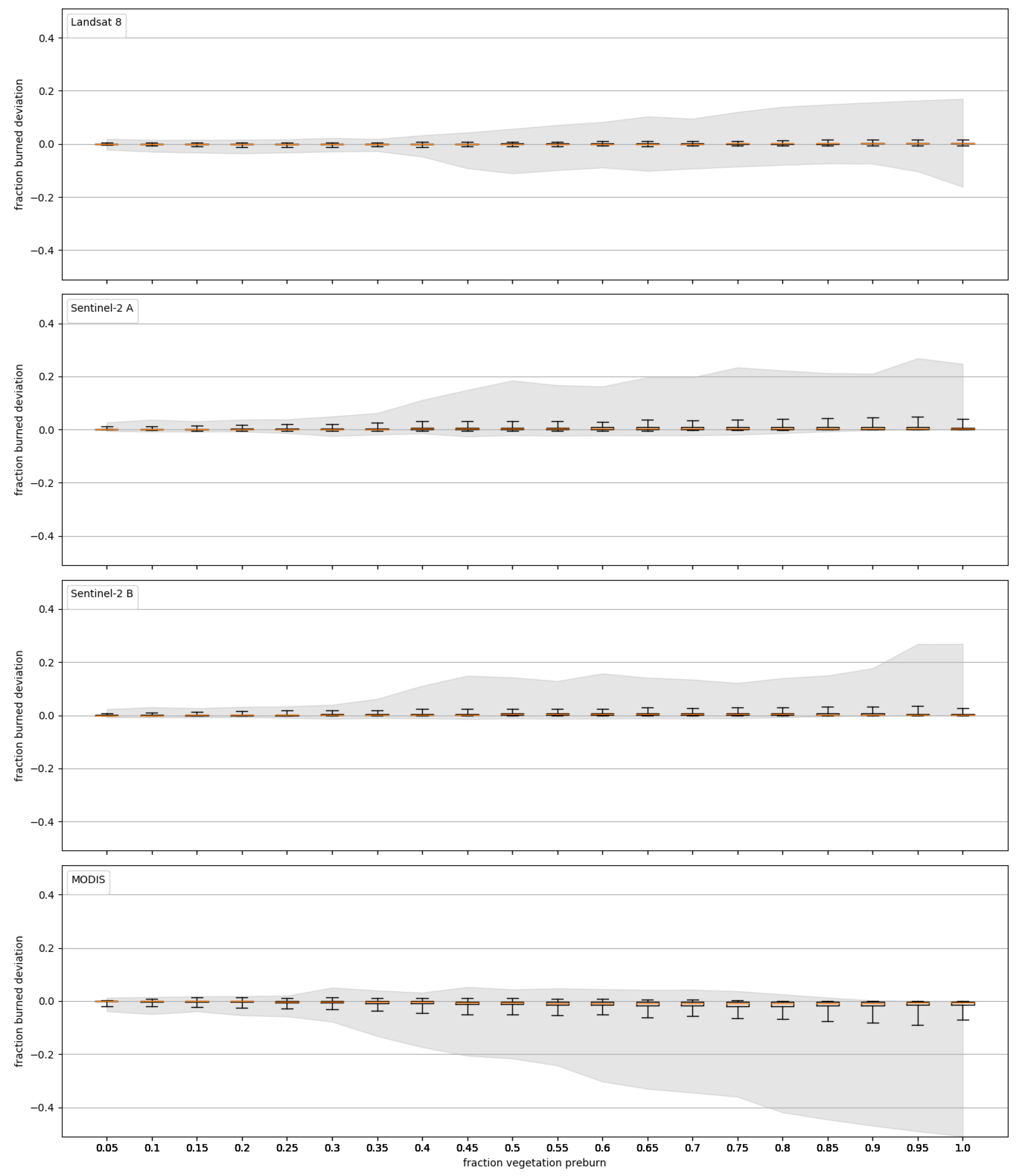
3.1. Differences between Satellite Sensors
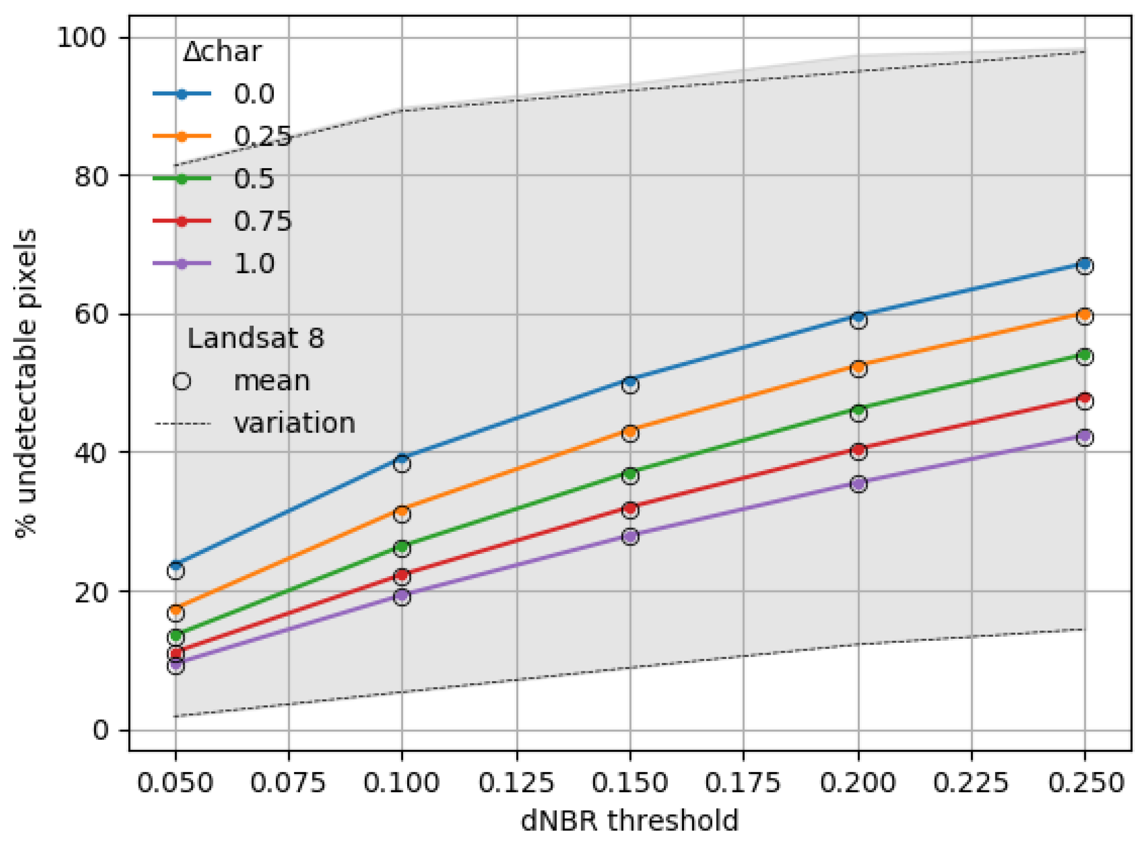
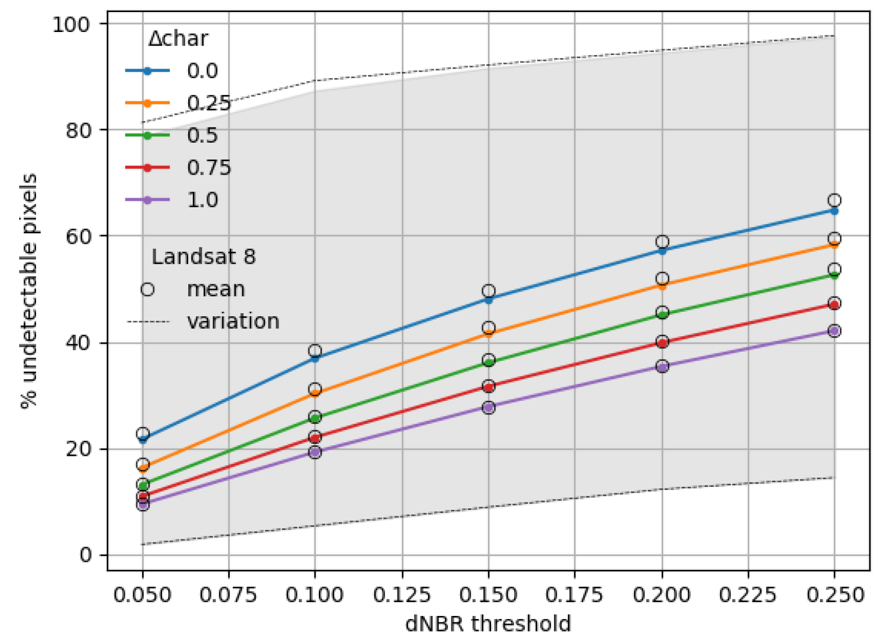
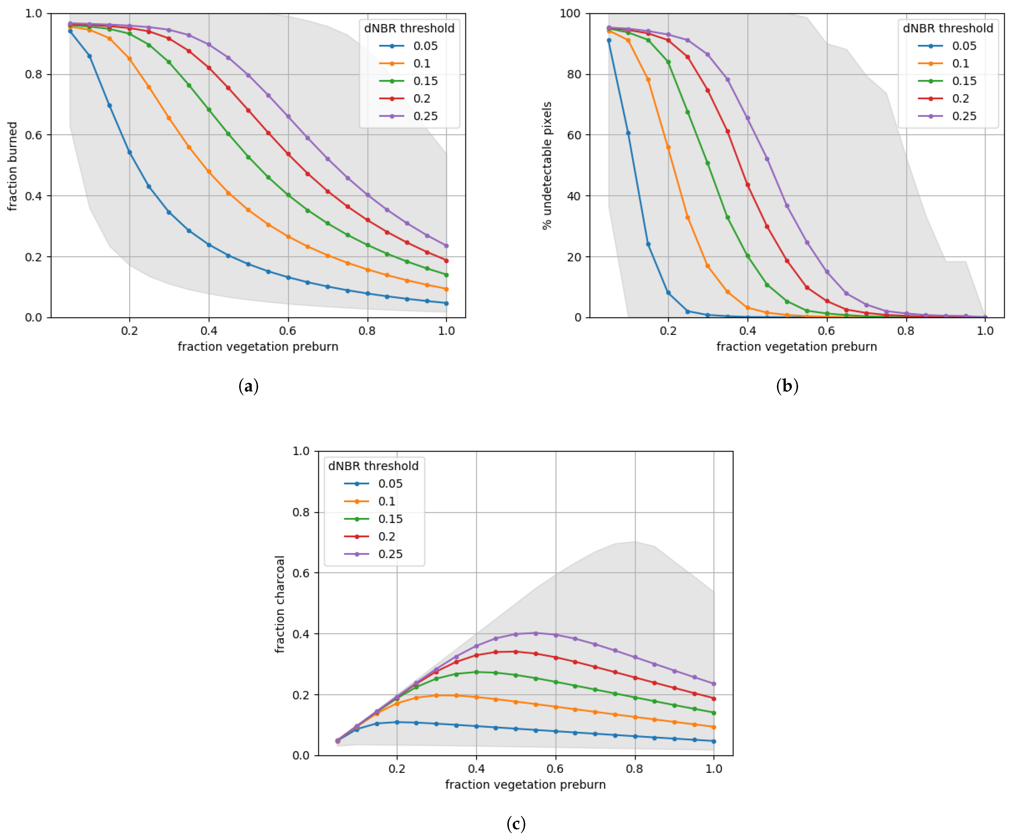
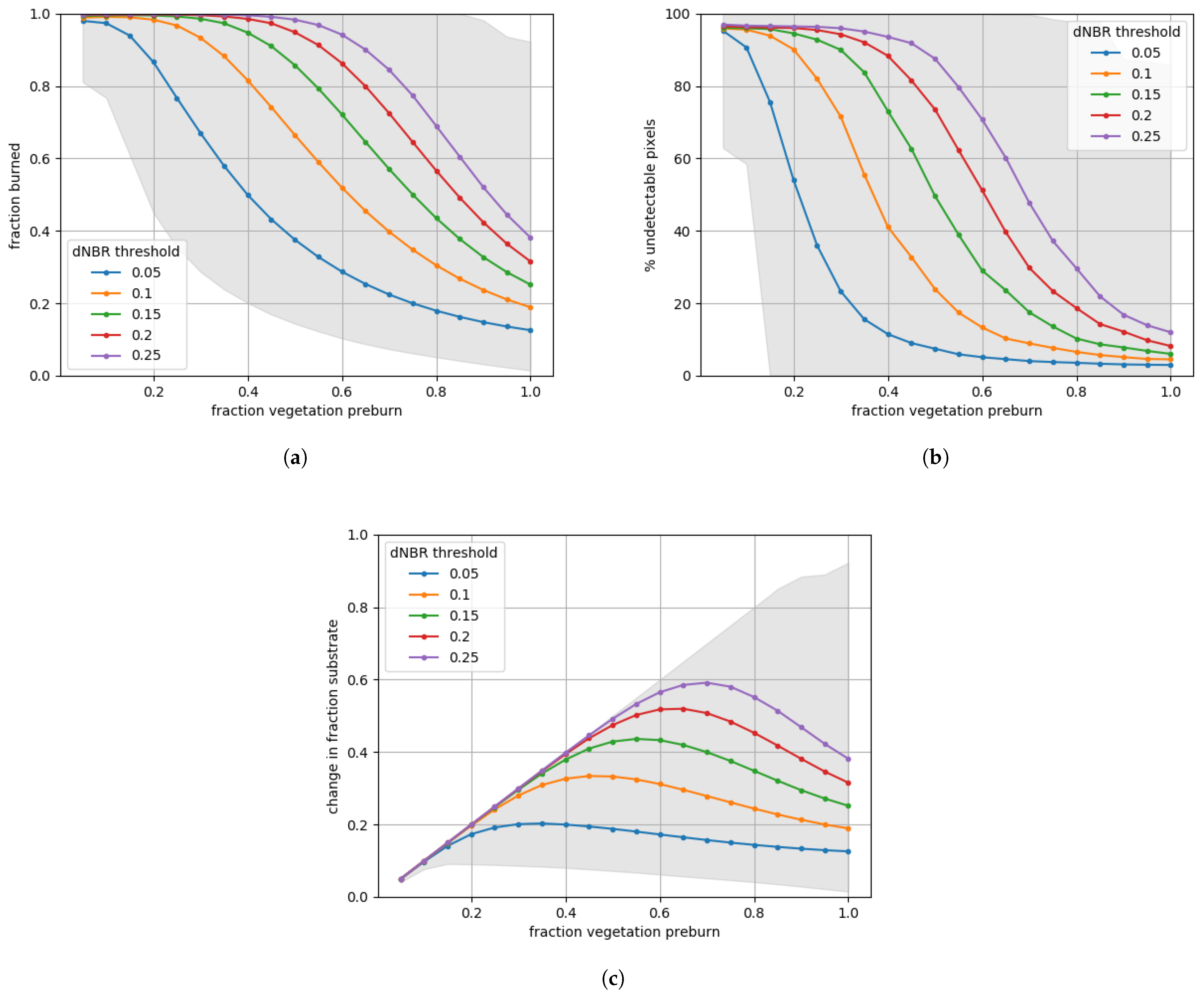
3.2. dNBR Threshold Influence
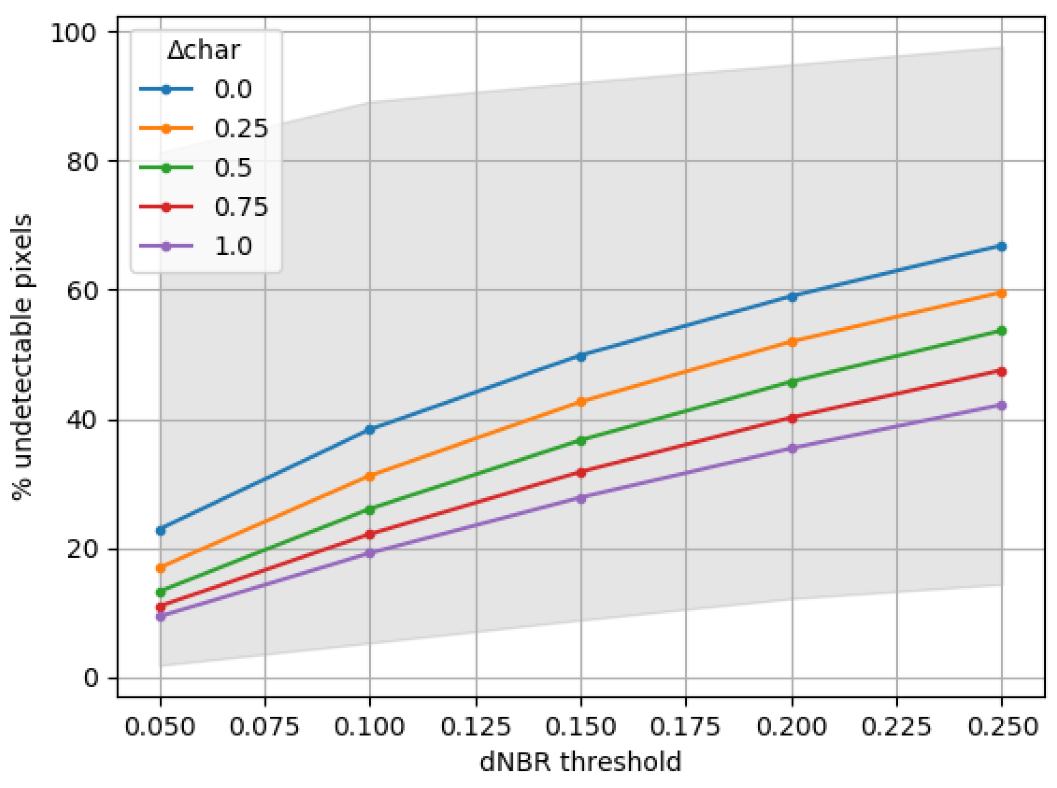
3.3. Park-Wide Detectability
4. Discussion
5. Conclusions
Author Contributions
Funding
Data Availability Statement
Acknowledgments
Conflicts of Interest
Abbreviations
| USA or U.S. | United States of America |
| NBR | Normalized Burn Ratio |
| dNBR | differenced Normalized Burn Ratio |
| RdNBR | Relative differenced Normalized Burn Ratio |
| NIR | Near-infrared |
| SWIR | Shortwave infrared |
| SMA | Spectral mixture analysis |
| USGS | United States Geological Survey |
| AVIRIS | Airborne Visible/Infrared Imaging Spectrometer |
| NASA | National Aeronautics and Space Administration |
| ECOSTRESS | Ecosystem Spaceborne Thermal Radiometer Experiment on Space Station |
| MODIS | Moderate Resolution Imaging Spectroradiometer |
Appendix A. Calculating Burned Fraction Directly

Appendix B. Results for Other Satellite Sensors
Appendix B.1. Results for Sentinel-2A


Appendix B.2. Results for Sentinel-2B


Appendix B.3. Results for MODIS


References
- Weber, M.G.; Flannigan, M.D. Canadian boreal forest ecosystem structure and function in a changing climate: Impact on fire regimes. Environ. Rev. 1997, 5, 145–166. [Google Scholar] [CrossRef]
- Stevens-Rumann, C.S.; Kemp, K.B.; Higuera, P.E.; Harvey, B.J.; Rother, M.T.; Donato, D.C.; Morgan, P.; Veblen, T.T. Evidence for declining forest resilience to wildfires under climate change. Ecol. Lett. 2018, 21, 243–252. [Google Scholar] [CrossRef] [PubMed]
- Shakesby, R.A.; Coelho, C.; Ferreira, A.D.; Terry, J.P.; Walsh, R.P. Wildfire impacts on soil-erosion and hydrology in wet Mediterranean forest, Portugal. Int. J. Wildland Fire 1993, 3, 95–110. [Google Scholar] [CrossRef]
- Abbate, A.; Longoni, L.; Ivanov, V.I.; Papini, M. Wildfire impacts on slope stability triggering in mountain areas. Geosciences 2019, 9, 417. [Google Scholar] [CrossRef] [Green Version]
- Van der Werf, G.R.; Randerson, J.T.; Giglio, L.; Leeuwen, T.T.V.; Chen, Y.; Rogers, B.M.; Mu, M.; Van Marle, M.J.; Morton, D.C.; Collatz, G.J.; et al. Global fire emissions estimates during 1997–2016. Earth Syst. Sci. Data 2017, 9, 697–720. [Google Scholar] [CrossRef] [Green Version]
- Reid, C.E.; Brauer, M.; Johnston, F.H.; Jerrett, M.; Balmes, J.R.; Elliott, C.T. Critical review of health impacts of wildfire smoke exposure. Environ. Health Perspect. 2016, 124, 1334–1343. [Google Scholar] [CrossRef] [Green Version]
- Liu, J.C.; Pereira, G.; Uhl, S.A.; Bravo, M.A.; Bell, M.L. A systematic review of the physical health impacts from non-occupational exposure to wildfire smoke. Environ. Res. 2015, 136, 120–132. [Google Scholar] [CrossRef] [Green Version]
- Doerr, S.H.; Santín, C. Global trends in wildfire and its impacts: Perceptions versus realities in a changing world. Philos. Trans. R. Soc. B Biol. Sci. 2016, 371, 20150345. [Google Scholar] [CrossRef]
- Wooster, M.J.; Roberts, G.J.; Giglio, L.; Roy, D.P.; Freeborn, P.H.; Boschetti, L.; Justice, C.; Ichoku, C.; Schroeder, W.; Davies, D.; et al. Satellite remote sensing of active fires: History and current status, applications and future requirements. Remote Sens. Environ. 2021, 267, 112694. [Google Scholar] [CrossRef]
- Martín, M.P.; Ceccato, P.; Flasse, S.; Downey, I. Fire detection and fire growth monitoring using satellite data. In Remote Sensing of Large Wildfires; Springer: Berlin/Heidelberg, Germany, 1999; pp. 101–122. [Google Scholar]
- Giglio, L.; Boschetti, L.; Roy, D.; Hoffmann, A.A.; Humber, M.; Hall, J.V. Collection 6 Modis Burned Area Product User’s Guide Version 1.0; NASA EOSDIS Land Processes DAAC: Sioux Falls, SD, USA, 2016.
- Roy, D.; Lewis, P.; Justice, C. Burned area mapping using multi-temporal moderate spatial resolution data—A bi-directional reflectance model-based expectation approach. Remote Sens. Environ. 2002, 83, 263–286. [Google Scholar] [CrossRef]
- Keshava, N.; Mustard, J.F. Spectral unmixing. IEEE Signal Process. Mag. 2002, 19, 44–57. [Google Scholar] [CrossRef]
- Ramo, R.; Roteta, E.; Bistinas, I.; Van Wees, D.; Bastarrika, A.; Chuvieco, E.; Van der Werf, G.R. African burned area and fire carbon emissions are strongly impacted by small fires undetected by coarse resolution satellite data. Proc. Natl. Acad. Sci. USA 2021, 118, e2011160118. [Google Scholar] [CrossRef] [PubMed]
- Loboda, T.; O’neal, K.; Csiszar, I. Regionally adaptable dNBR-based algorithm for burned area mapping from MODIS data. Remote Sens. Environ. 2007, 109, 429–442. [Google Scholar] [CrossRef]
- Picotte, J.J.; Robertson, K. Timing constraints on remote sensing of wildland fire burned area in the southeastern US. Remote Sens. 2011, 3, 1680–1690. [Google Scholar] [CrossRef] [Green Version]
- Kolden, C.A.; Lutz, J.A.; Key, C.H.; Kane, J.T.; van Wagtendonk, J.W. Mapped versus actual burned area within wildfire perimeters: Characterizing the unburned. For. Ecol. Manag. 2012, 286, 38–47. [Google Scholar] [CrossRef]
- Hawbaker, T.J.; Vanderhoof, M.K.; Schmidt, G.L.; Beal, Y.J.; Picotte, J.J.; Takacs, J.D.; Falgout, J.T.; Dwyer, J.L. The Landsat Burned Area algorithm and products for the conterminous United States. Remote Sens. Environ. 2020, 244, 111801. [Google Scholar] [CrossRef]
- Roteta, E.; Bastarrika, A.; Padilla, M.; Storm, T.; Chuvieco, E. Development of a Sentinel-2 burned area algorithm: Generation of a small fire database for sub-Saharan Africa. Remote Sens. Environ. 2019, 222, 1–17. [Google Scholar] [CrossRef]
- García, M.L.; Caselles, V. Mapping burns and natural reforestation using Thematic Mapper data. Geocarto Int. 1991, 6, 31–37. [Google Scholar] [CrossRef]
- Key, C.; Benson, N. Landscape assessment: Remote sensing of severity, the normalized burn ratio and ground measure of severity, the composite burn index. In FIREMON: Fire Effects Monitoring and Inventory System Ogden; USDA Forest Service, Rocky Mountain Research Station: Ogden, UT, USA, 2005. [Google Scholar]
- Somers, B.; Asner, G.P.; Tits, L.; Coppin, P. Endmember variability in spectral mixture analysis: A review. Remote Sens. Environ. 2011, 115, 1603–1616. [Google Scholar] [CrossRef]
- Veraverbeke, S.; Hook, S.J. Evaluating spectral indices and spectral mixture analysis for assessing fire severity, combustion completeness and carbon emissions. Int. J. Wildland Fire 2013, 22, 707–720. [Google Scholar] [CrossRef]
- Tane, Z.; Roberts, D.; Veraverbeke, S.; Casas, Á.; Ramirez, C.; Ustin, S. Evaluating endmember and band selection techniques for multiple endmember spectral mixture analysis using post-fire imaging spectroscopy. Remote Sens. 2018, 10, 389. [Google Scholar] [CrossRef] [Green Version]
- Eckmann, T.C.; Roberts, D.A.; Still, C.J. Using multiple endmember spectral mixture analysis to retrieve subpixel fire properties from MODIS. Remote Sens. Environ. 2008, 112, 3773–3783. [Google Scholar] [CrossRef]
- Veraverbeke, S.; Gitas, I.; Katagis, T.; Polychronaki, A.; Somers, B.; Goossens, R. Assessing post-fire vegetation recovery using red–near infrared vegetation indices: Accounting for background and vegetation variability. ISPRS J. Photogramm. Remote Sens. 2012, 68, 28–39. [Google Scholar] [CrossRef] [Green Version]
- U.S. Department of the Interior; National Park Service. Yellowstone National Park. 2020. Available online: https://www.nps.gov/yell/index.htm (accessed on 21 September 2021).
- Rodman, A.W.; Shovic, H.F.; Thoma, D.P. Soils of Yellowstone National Park; Yellowstone Center for Resources, National Park Service: Yellowstone National Park, WY, USA, 1996.
- Richmond, G.M. Stratigraphy and chronology of glaciations in Yellowstone National Park. Quat. Sci. Rev. 1986, 5, 83–98. [Google Scholar] [CrossRef]
- Henne, P.D.; Hawbaker, T.J.; Scheller, R.M.; Zhao, F.; He, H.S.; Xu, W.; Zhu, Z. Increased burning in a warming climate reduces carbon uptake in the Greater Yellowstone Ecosystem despite productivity gains. J. Ecol. 2021, 109, 1148–1169. [Google Scholar] [CrossRef]
- Kokaly, R.; Clark, R.; Swayze, G.; Livo, K.; Hoefen, T.; Pearson, N.; Wise, R.; Benzel, W.; Lowers, H.; Driscoll, R.; et al. Usgs Spectral Library Version 7 Data: Us Geological Survey Data Release; United States Geological Survey (USGS): Reston, VA, USA, 2017.
- Meerdink, S.K.; Hook, S.J.; Roberts, D.A.; Abbott, E.A. The ECOSTRESS spectral library version 1.0. Remote Sens. Environ. 2019, 230, 111196. [Google Scholar] [CrossRef]
- Keefer, W.R. The Geologic Story of Yellowstone National Park; US Government Printing Office: Washington, DC, USA, 1971; Volume 1347.
- Demattê, J.A.; da Silva Terra, F. Spectral pedology: A new perspective on evaluation of soils along pedogenetic alterations. Geoderma 2014, 217, 190–200. [Google Scholar] [CrossRef]
- Smith, A.M.; Eitel, J.U.; Hudak, A.T. Spectral analysis of charcoal on soils: Implicationsfor wildland fire severity mapping methods. Int. J. Wildland Fire 2010, 19, 976–983. [Google Scholar] [CrossRef]
- Soil Survey Staff. Illustrated Guide to Soil Taxonomy, Version 2; U.S. Department of Agriculture, Natural Resources Conservation Service, National Soil Survey Center: Lincoln, NE, USA, 2015.
- Veraverbeke, S.; Hook, S.J.; Harris, S. Synergy of VSWIR (0.4–2.5 μm) and MTIR (3.5–12.5 μm) data for post-fire assessments. Remote Sens. Environ. 2012, 124, 771–779. [Google Scholar] [CrossRef]
- Barsi, J.A.; Lee, K.; Kvaran, G.; Markham, B.L.; Pedelty, J.A. The spectral response of the Landsat-8 operational land imager. Remote Sens. 2014, 6, 10232–10251. [Google Scholar] [CrossRef] [Green Version]
- U.S. Department of the Interior; U.S. Geological Survey. Landsat 8. 2013. Available online: https://www.usgs.gov/core-science-systems/nli/landsat/landsat-8?qt-science_support_page_related_con=0#qt-science_support_page_related_con (accessed on 21 October 2021).
- ESA. Sentinel-2 MSI Technical Guide. 2018. Available online: https://sentinel.esa.int/web/sentinel/technical-guides/sentinel-2-msi (accessed on 21 October 2021).
- NASA. MODIS Data. 2012. Available online: https://modis.gsfc.nasa.gov/data/ (accessed on 21 October 2021).
- Quintano, C.; Fernández-Manso, A.; Shimabukuro, Y.E.; Pereira, G. Spectral unmixing. Int. J. Remote Sens. 2012, 33, 5307–5340. [Google Scholar] [CrossRef]
- U.S. Department of the Interior; U.S. Geological Survey. Digital Geologic Map of Yellowstone National Park, Idaho, Montana, and Wyoming and Vicinity. 1999. Available online: https://pubs.usgs.gov/of/1999/ofr-99-0174/ (accessed on 2 January 2022).
- Despain, D.G. Yellowstone Vegetation: Consequences of Environment and History in a Natural Setting; Roberts Rinehart Publishers: Boulder, CO, USA, 1990. [Google Scholar]
- Randerson, J.; Chen, Y.; Van Der Werf, G.; Rogers, B.; Morton, D. Global burned area and biomass burning emissions from small fires. J. Geophys. Res. Biogeosci. 2012, 117, G04. [Google Scholar] [CrossRef]
- Glushkov, I.; Zhuravleva, I.; McCarty, J.L.; Komarova, A.; Drozdovsky, A.; Drozdovskaya, M.; Lupachik, V.; Yaroshenko, A.; Stehman, S.V.; Prishchepov, A.V. Spring fires in Russia: Results from participatory burned area mapping with Sentinel-2 imagery. Environ. Res. Lett. 2021, 16, 125005. [Google Scholar] [CrossRef]
- Cui, W.; Perera, A.H. What do we know about forest fire size distribution, and why is this knowledge useful for forest management? Int. J. Wildland Fire 2008, 17, 234–244. [Google Scholar] [CrossRef]
- Sunderman, S.O.; Weisberg, P.J. Remote sensing approaches for reconstructing fire perimeters and burn severity mosaics in desert spring ecosystems. Remote Sens. Environ. 2011, 115, 2384–2389. [Google Scholar] [CrossRef]
- Somers, B.; Cools, K.; Delalieux, S.; Stuckens, J.; Van der Zande, D.; Verstraeten, W.W.; Coppin, P. Nonlinear hyperspectral mixture analysis for tree cover estimates in orchards. Remote Sens. Environ. 2009, 113, 1183–1193. [Google Scholar] [CrossRef]
- Miller, J.D.; Thode, A.E. Quantifying burn severity in a heterogeneous landscape with a relative version of the delta Normalized Burn Ratio (dNBR). Remote Sens. Environ. 2007, 109, 66–80. [Google Scholar] [CrossRef]
- Roy, D.P.; Huang, H.; Boschetti, L.; Giglio, L.; Yan, L.; Zhang, H.H.; Li, Z. Landsat-8 and Sentinel-2 burned area mapping-A combined sensor multi-temporal change detection approach. Remote Sens. Environ. 2019, 231, 111254. [Google Scholar] [CrossRef]
- Roy, D.P.; Landmann, T. Characterizing the surface heterogeneity of fire effects using multi-temporal reflective wavelength data. Int. J. Remote Sens. 2005, 26, 4197–4218. [Google Scholar] [CrossRef]
- Stroppiana, D.; Bordogna, G.; Carrara, P.; Boschetti, M.; Boschetti, L.; Brivio, P. A method for extracting burned areas from Landsat TM/ETM+ images by soft aggregation of multiple Spectral Indices and a region growing algorithm. ISPRS J. Photogramm. Remote Sens. 2012, 69, 88–102. [Google Scholar] [CrossRef]
- Storey, E.A.; Lee West, K.R.; Stow, D.A. Utility and optimization of LANDSAT-derived burned area maps for southern California. Int. J. Remote Sens. 2021, 42, 486–505. [Google Scholar] [CrossRef]


| Type | Vegetation Community | Dominant Species | No. of Samples |
|---|---|---|---|
| Forest | Douglas fir | Pseudotsuga menziesii | 3 |
| Lodgepole pine | Pinus contorta subsp. latifolia | 11 | |
| Spruce fir | Picea engelmannii, Abies lasiocarpa | 5 | |
| Whitebark pine | Pinus albicaulis | 2 | |
| Nonforest | Bacterial mat | Chloroflexus aurantiacus, Synechococcus lividus | 1 |
| Conifer–meadow mix | 1 | ||
| Grass | Festuca idahoensis | 5 | |
| Sagebrush | Artemisia tridentata | 4 | |
| Sedge | 1 | ||
| Willow–sedge mix | 1 |
| Geological Unit | Rock/Soil Name | No. of Samples |
|---|---|---|
| Precambrian Gneiss and Schist | Gneiss | 19 |
| Schist | 26 | |
| Inceptisol dystrochrept | 1 | |
| Inceptisol haplumbrept | 1 | |
| Paleozoic Formations | Dolomite | 3 |
| Limestone | 33 | |
| Sandstone | 21 | |
| Shale | 25 | |
| Mesozoic Formations | Limestone | 33 |
| Sandstone | 21 | |
| Shale | 25 | |
| Tertiary Formations | Conglomerate | 3 |
| Sandstone | 21 | |
| Diorite Intrusions | Diorite | 2 |
| Granodiorite | 4 | |
| Absaroka Volcanic Breccias | Andesite | 6 |
| Basalt | 35 | |
| Mafic tuff | 1 | |
| Inceptisol haplumbrept | 1 | |
| Mollisol cryoboroll | 1 | |
| Yellowstone Tuffs | Felsic tuff | 8 |
| Alfisol fragiboralf | 1 | |
| Alfisol haplustalf | 2 | |
| Inceptisol xerumbrept | 1 | |
| Plateau Rhyolite | Rhyolite | 24 |
| Inceptisol cryumbrept | 1 | |
| Inceptisol plaggept | 1 | |
| Mollisol cryoboroll | 1 | |
| Basalt Flows | Basalt | 35 |
| Quartenary Deposits | Travertine | 2 |
| Alfisol fragiboralf | 1 | |
| Alfisol haplustalf | 2 | |
| Alfisol paleustalf | 1 | |
| Inceptisol cryumbrept | 1 | |
| Inceptisol haplumbrept | 1 | |
| Inceptisol plaggept | 1 | |
| Inceptisol xerumbrept | 1 | |
| Mollisol cryoboroll | 1 | |
| Mollisol haplustall | 1 |
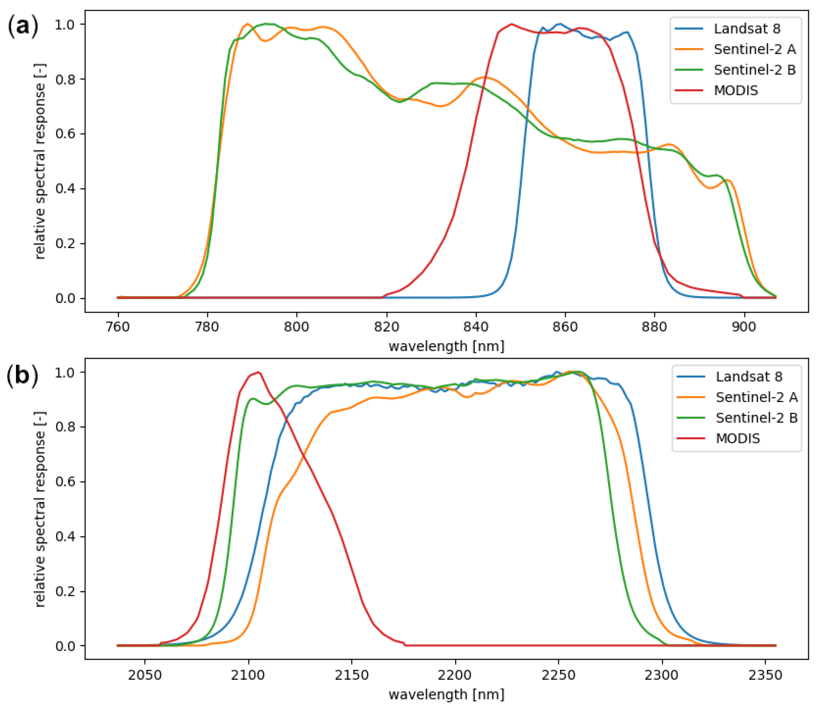
| NIR Band | SWIR Band | ||||||
|---|---|---|---|---|---|---|---|
| Satellite Instrument | Band No. | Range (m) | Resolution (m) | Band No. | Range (m) | Resolution (m) | Data Source |
| Landsat 8 | 5 | 0.85–0.88 | 30 | 7 | 2.11–2.29 | 30 | [39] |
| Sentinel-2 A & B | 8 | 0.78–0.89 | 10 | 12 | 2.01–2.37 | 20 | [40] |
| MODIS Terra & Aqua | 2 | 0.84–0.89 | 250 | 7 | 2.11–2.16 | 500 | [41] |
| Level | Name | Results Count | Notes |
|---|---|---|---|
| 0 | Endmembers | 49,572,000 | Results are not saved at this level. |
| 1 | Groupings | 1,170,000 | Contains min, mean, and max values of sample combination groupings. |
| 2 | Geologies | 300,000 | Substrate groupings aggregated to their geological units. |
| 3 | Park-wide | 6000 | Weighted average using abundances of geology–vegetation combinations. |
| Douglas Fir | Lodgepole Pine | Spruce Fir | Whitebark Pine | Nonforest | Total | |
|---|---|---|---|---|---|---|
| Precambrian Formations | 0.675 | 0.607 | 0.007 | 0.130 | 0.517 | 1.94 |
| Paleozoic Formations | 0.141 | 0.653 | 0.038 | 0.344 | 0.509 | 1.69 |
| Mesozoic Formations | 0.106 | 0.919 | 0.234 | 0.749 | 0.694 | 2.70 |
| Tertiary Formations | 0 | 0.002 | 0 | 0.001 | 0.001 | 0.003 |
| Diorite Intrusions | 0.081 | 0.079 | 0.005 | 0.148 | 0.236 | 0.549 |
| Absaroka Volcanics | 1.18 | 5.74 | 0.842 | 7.63 | 5.78 | 21.2 |
| Yellowstone Tuffs | 0.826 | 10.8 | 1.26 | 1.09 | 0.519 | 14.5 |
| Plateau Rhyolite | 0.073 | 18.8 | 1.74 | 2.14 | 1.75 | 24.5 |
| Basalt Flows | 0.230 | 1.39 | 0.045 | 0.039 | 0.145 | 1.86 |
| Quartenary Deposits | 1.11 | 13.4 | 6.30 | 1.97 | 8.25 | 31.0 |
| total | 4.42 | 52.5 | 10.5 | 14.2 | 18.4 | 100 |
Publisher’s Note: MDPI stays neutral with regard to jurisdictional claims in published maps and institutional affiliations. |
© 2022 by the authors. Licensee MDPI, Basel, Switzerland. This article is an open access article distributed under the terms and conditions of the Creative Commons Attribution (CC BY) license (https://creativecommons.org/licenses/by/4.0/).
Share and Cite
Riet, M.; Veraverbeke, S. How Much of a Pixel Needs to Burn to Be Detected by Satellites? A Spectral Modeling Experiment Based on Ecosystem Data from Yellowstone National Park, USA. Remote Sens. 2022, 14, 2075. https://doi.org/10.3390/rs14092075
Riet M, Veraverbeke S. How Much of a Pixel Needs to Burn to Be Detected by Satellites? A Spectral Modeling Experiment Based on Ecosystem Data from Yellowstone National Park, USA. Remote Sensing. 2022; 14(9):2075. https://doi.org/10.3390/rs14092075
Chicago/Turabian StyleRiet, Mats, and Sander Veraverbeke. 2022. "How Much of a Pixel Needs to Burn to Be Detected by Satellites? A Spectral Modeling Experiment Based on Ecosystem Data from Yellowstone National Park, USA" Remote Sensing 14, no. 9: 2075. https://doi.org/10.3390/rs14092075
APA StyleRiet, M., & Veraverbeke, S. (2022). How Much of a Pixel Needs to Burn to Be Detected by Satellites? A Spectral Modeling Experiment Based on Ecosystem Data from Yellowstone National Park, USA. Remote Sensing, 14(9), 2075. https://doi.org/10.3390/rs14092075