Spatial Sampling and Grouping Information Entropy Strategy Based on Kernel Fuzzy C-Means Clustering Method for Hyperspectral Band Selection

Abstract

The high spectral resolution of hyperspectral images (HSIs) provides rich information but causes data redundancy, which imposes a computational burden on practical applications. Band selection methods can select a subset of HSI without changing the main information to reduce the spectral dimension. Clustering-based methods can reduce band correlation significantly, but traditional clustering methods are mostly hard clustering and are not accurate enough to partition the bands. An unsupervised band selection method based on fuzzy c-means clustering (FCM) was introduced to tackle this problem. However, FCM can easily obtain the local optimal solution and take a long time to process high-dimensional data. Hence, this work applies kernel function and a sampling strategy to reduce calculation time, and information entropy is used to initialize the cluster center. A kernel FCM algorithm based on spatial sampling and a grouping information entropy strategy is proposed and called SSGIE-KFCM. This method not only optimizes the calculation process and reduces the amount of computation data, accelerating the calculation efficiency, but also adopts grouping information entropy to improve the probability of obtaining a global optimal solution. Classification experiments on two public HSI datasets show that: (1) The classification performance of the whole band can be achieved or even exceeded by using only a small number of bands to achieve the purpose of dimensionality reduction. (2) The classification accuracy can be improved compared with the FCM method. (3) With the introduction of sampling strategy and kernel function, the computational speed is at least 24 times faster than that of FCM. It has been proven that the SSGIE-KFCM method can significantly reduce the amount of HSI while retaining the primary information of the original data, which further promotes the research and application of HSI in the remote sensing area.

1. Introduction

In recent years, hyperspectral image (HSI) processing has become a hot spot in the remote sensing field [1,2]. Compared with multispectral images, HSI has a higher spectral resolution and can obtain images with more channels. Spectral values at the exact location can form continuous spectral curves to enhance the discriminatory ability of ground objects [3,4]. Due to subtle spectral resolution, more detailed spectral characteristics of the pixels are obtained. As the amount of information of HSI increases, data transmission and subsequent processing time increase, which reduces the application efficiency. Moreover, it is necessary to reduce the dimension before using the HSI data because of the high correlation and dependence among adjacent bands, resulting in large computational complexity and the Hughes’ phenomenon [5].

At present, two main methods of dimensionality reduction exist. One is feature extraction, and the other is band selection [6], also known as feature selection. Feature extraction converts the original data from high-dimensional data to low-dimensional data through operations, such as principal component analysis (PCA) [7], independent component analysis (ICA) [8], discrete wavelet transform (DWT) [9], etc., which changes the physical information of the original data. However, this information plays an important role in practical applications such as classification [10,11], target detection [12,13,14,15], anomaly detection [16,17,18], spectral unmixing [19,20], hyperspectral image restoration [21,22,23,24,25,26], and hyperspectral compressive sensing [27].Band selection involves selecting a certain number of bands as a representative subset from all bands according to specific rules. These subsets can represent the original HSI information. Relative to the feature extraction method, the physical significance of each band value of the original data can be retained to meet specific application needs.

Band selection can be divided into supervised, semisupervised, and unsupervised methods according to the degree of prior information participation [28,29]. Labeled information is used by supervised and semisupervised methods to improve the quality of selection results to some extent, but in practice, obtaining prior information is difficult, so unsupervised methods are more feasible than the above two methods.

According to the algorithm principle, band selection can be divided into (1) the sparse-based method, (2) the search-based method, (3) the ranking-based method, (4) the clustering-based method, and (5) the mixing-based method, which combines the above methods. The clustering-based method considers each band as an object and divides all bands into several clusters, which maximizes the distance between the cluster centers and minimizes the distance between objects within clusters. It then selects a representative band from each cluster to form a subset, effectively reducing the similarity between the extracted bands.

Furthermore, traditional clustering-based methods mostly comprise hard clustering, i.e., when an object belongs to a particular class, it is in an either/or position. However, due to the complexity of spectral information in HSIs, a band may belong to different clusters concurrently. The hard clustering method is not accurate enough for object partitioning, but the fuzzy clustering-based method, which calculates the object’s membership to each class, can satisfactorily resolve this issue [30]. The fuzzy c-means clustering (FCM) [31] method is an iterative soft clustering method. In the process of clustering, objects are not simply divided into one class, but the probability of attributing objects to all classes is calculated, allowing samples to belong to multiple clusters at different probabilities simultaneously.

Nevertheless, the whole computing procedure takes a long time for data with higher dimensions to obtain results. Moreover, the random initialization process easily leads to FCM falling into the local optimal solution. Havens and Bezdek et al. [32] employed the kernel FCM (KFCM) method for very large data, transforming the data into reproducing kernel Hilbert space (RKHS) to simplify the calculation process and improve efficiency. Therefore, this paper adopts KFCM for band selection. In addition, it uses spatial sampling and grouping information entropy strategies to simplify the input data and tackle the local optimal solution problem, respectively. Finally, a novel method called SSGIE-KFCM is presented. The contributions of this paper are given as follows:

(1) The KFCM algorithm is innovatively introduced into the field of hyperspectral band selection, and FCM is modified using a kernel function to optimize the iterative calculation process, reducing the computational complexity. To our knowledge, kernel clustering has not yet been utilized in band selection.

(2) A simple and effective sampling strategy is proposed. Sampling HSI data in the spatial dimension ensures that the spatial distribution remains approximately invariant. It can reduce the amount of data by half and the calculation time with little or no influence on the results.

(3) The information entropy of each band is calculated, and the bands with higher information entropy values are selected by grouping instead of globally, which is used as the initial cluster center, further tackling the problem of trapping into local optimums in FCM.

The rest of this article is arranged as follows. Section 2 describes the related work of band selection methods. In Section 3, the process and details of the proposed method are presented. The experimental results on the public HSI dataset are shown in Section 4, and Section 5 summarizes this paper.

2. Related Work

The principle of matrix decomposition is used in the sparse-based method. First, the three-dimensional HSI cube H is transformed into a two-dimensional matrix X. Then, X is divided into matrix A and Z via sparse decomposition, where A is called the characteristic matrix, also known as the dictionary, and Z is the coefficient matrix. Sparse coefficients reveal the potential structure of HSI, so the final band subset can be found by computing the coefficient matrix. In 2011, Li et al. [33] used the K-SVD algorithm to calculate the characteristic matrix and the coefficient matrix, then sorted each column of the coefficient matrix Z in descending order and selected the first k items of each column to form the matrix Z_s. The histogram of Z_s shows the frequency of each band in Z_s. The k most frequently occurring indices are selected according to the histogram, and the corresponding bands of the original HSI are selected as the final band subset. In the same year, Li et al. [34] introduced the sparse non-negative matrix factorization (SNMF) method into band selection, but the disadvantage of this method is that there is no unique solution to the band index obtained. That is, the results are not the same each time. Moreover, Sun et al. [35] proposed an improved sparse space clustering (ISSC) algorithm inspired by sparse space clustering to optimize the sparse matrix through the L₂ norm.

The search-based method converts the band selection into an optimization problem of a criterion function. Generally, it is difficult or impossible to solve a given criterion function. A local or global optimal solution can be obtained if a search method is adopted to optimize the criterion function. Therefore, the search-based approach has two critical points: (1) criterion functions and (2) search strategies. Sequential forward search (SFS) [36], proposed by Whitney in 1971, is an earlier method that searched for an additional band based on the bands already selected. This method yielded a suboptimal solution and suffered from the so-called “nesting effect” [37]. In 2016, Su et al. [38] used minimum estimated abundance covariance (MEAC) distance and Jeffries–Matusita (JM) distance as objective functions, respectively. Then, the Firefly algorithm, a swarm intelligence algorithm, was used to search for the optimal solution, resulting in two band selection algorithms. All the above methods optimize the single objective function. Subsequently, Gong et al. [39] designed two conflicting objective functions, one for information entropy and the other for the number of selected bands. Both are required to be minimized simultaneously in the conflicted relationship. A multiobjective evolutionary algorithm (MOEA) is presented to solve this problem. Within the framework of this model, band subsets of different band numbers can be collaboratively optimized. They can communicate with each other by interchanging bands and improve the quality of results by using the relationship between the band subsets of different band numbers. This selection method is named multiobjective optimization band selection (MOBS).

The basic idea of the ranking-based method is to use an evaluation criterion to score each band, rank the score from high to low, and select the top bands as band subsets. In 1999, Chang et al. [40] proposed a maximum-variance principal component analysis (MVPCA) method for band selection based on the decomposition of matrix features (spectral). This method calculated the variance of each band and selected several bands with the most significant variance. However, the bands selected by this method have correlation, and information is still redundant. Kim et al. [41] employed the covariance of the background data to evaluate the effect of bands on the detection performance of the matched filter (MF) and adaptive coherence estimator (ACE), and sorted and selected the band subset with greater influence. Then, they applied it in near real-time target detection. Although the ranking-based method can select bands with a high amount of information, the selected band subset may have correlation, and the characteristics of the clustering-based algorithm can avoid this problem.

The earliest band selection methods based on the clustering idea are Ward’s linkage strategy using mutual information (WaLuMI) and Ward’s linkage strategy using divergence (WaLuDI), proposed by Adolfo et al. [42] in 2007, which is a hierarchical clustering algorithm based on Ward’s linkage. In 2009, Qian et al. [43] designed an unsupervised method, the affinity propagation (AP) algorithm; Su et al. [44] then developed a sample-based semisupervised adaptive AP. Afterwards, Yang et al. [45] proposed a representative band-mining method based on k-means clustering. Yuan et al. [46] extended the k-means clustering algorithm to a dual-clustering method using context analysis. The above two methods belong to hard clustering. In 2017, Zhang et al. [30] used the FCM method for band selection. They introduced a particle swarm optimization (PSO) algorithm for the local optimal solution problem to search globally and obtain a global optimal solution. The experiments show that PSO can effectively improve the classification accuracy of selected bands. Because the whole calculation process of PSO replaces one of the cluster centers, it increases the amount of calculation, but finding the global optimal solution faster can reduce the number of iterations. Consequently, in terms of execution efficiency, the introduction of PSO does not guarantee that the entire time will be shortened. Even with a large amount of HSI data, it may increase the running time too much.

This paper is also based on the FCM method for band selection, but unlike the idea in ref. [30], we adopted the kernel function to modify the FCM. Before iterative optimization, the spatial sampling strategy is employed to reduce the amount of data and improve the operating efficiency. The initial cluster center is selected by using grouping information entropy to address the issue of the local optimal solution.

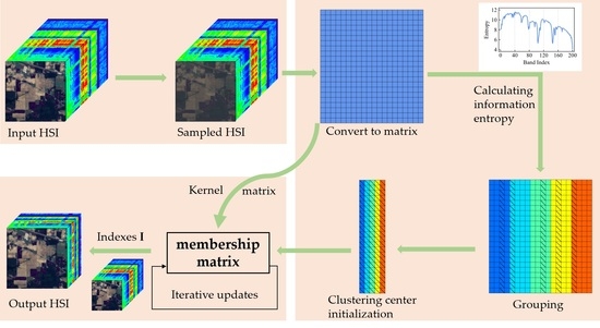
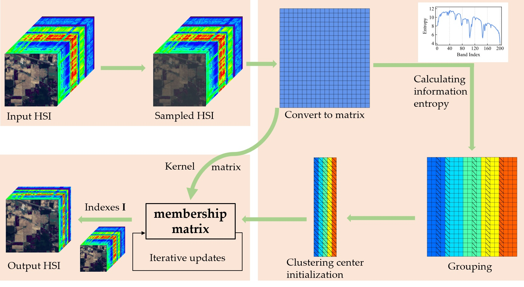
3. Proposed Method

The flowchart of the proposed SSGIE-KFCM method is shown in Figure 1. To better understand the calculation of hyperspectral band selection, we first define some of the symbols used in this paper. Let $H\in {ℝ}^{a\times b\times n}$ represent HSI data, where a and b are the number of rows and columns in the spatial dimension of a single-band image, and n is the number of bands of HSI. Let ${\mathbf{h}}_i\in {ℝ}^{a\times b}$ denote the ith band image. Usually, in the calculation process, $H$ is first converted into a two-dimensional matrix, denoted as $\mathbf{X}\in {ℝ}^{g\times n}$, where g = a × b, and ${\mathbf{x}}_i\in {ℝ}^g$ is the ith column vector of X (i.e., the ith band vector).

3.1. Fuzzy C-Means Clustering Method

The FCM algorithm calculates the membership degree of each object in different subsets and divides the object into the corresponding cluster with the most significant membership value. The determination of each membership value can be defined as the following optimization problem:

$$\begin{array}{l}\underset{u_{ij}}{\min }\hspace{1em}J={\displaystyle \sum _{i=1}^n{\displaystyle \sum _{j=1}^m{u}_{ij}^q{d}_{ij}^2}}\\ \mathrm{s}.\mathrm{t}. \left\{\begin{array}{l}{u}_{ij}\in \left[0,1\right]\\ {\displaystyle {\sum }_{j=1}^m{u}_{ij}=1,\hspace{1em}\forall i=1, 2, \dots , n}\end{array}\right.\end{array}$$

(1)

$$d_{ij}=‖c_j-x_i‖$$

(2)

where n and m are the total number of clustering objects and clustering subsets; u_ij denotes the membership degree of the ith object x_i to the jth class. From the actual physical meaning, the sum of the membership values of an object to all classes is 1. d_ij stands for the Euclidean distance between the ith object x_i and the jth cluster center c_j, and q is the weighted index of the controlling membership within the range [1, ∞), usually 2.

For Equation (1), the Lagrange multiplier method can be used to solve this problem as follows:

$$\overline{J}={\displaystyle \sum _{i=1}^n{\displaystyle \sum _{j=1}^m{u}_{ij}^q{d}_{ij}^2}}+{\displaystyle \sum _{i=1}^n{\lambda }_i\left({\displaystyle \sum _{j=1}^m{u}_{ij}-1}\right)}$$

(3)

The partial derivative of $\overline{J}$ with respect to u_ij is taken and made equal to 0. Then, according to the constraints of u_ij, the formula for calculating membership values can be derived:

$$u_{ij}={\left[{\displaystyle \sum _{o=1}^m{\left(\frac{‖c_j-x_i‖}{‖c_o-x_i‖}\right)}^{\frac{2}{q-1}}}\right]}^{-1}$$

(4)

Then, Equation (4) is brought into Equation (3). The partial derivative of $\overline{J}$ with respect to c_j is calculated and made equal to 0. The cluster center can be calculated and expressed as

$$c_j=\frac{{\displaystyle {\sum }_{i=1}^n{u}_{ij}^q{x}_i}}{{\displaystyle {\sum }_{i=1}^n{u}_{ij}^q}}$$

(5)

Equation (4) shows that when calculating the membership degree, the coordinates of the cluster centers need to be known, while when c_j is calculated by Equation (5), u_ij needs to be calculated first. Accordingly, a membership matrix $\mathbf{U}\in {ℝ}^{n\times m}$ that satisfies the constraints of u_ij is randomly initialized, and then the cluster center matrix $\mathbf{C}=\left[{\mathbf{c}}_1,{\mathbf{c}}_2,\dots ,{\mathbf{c}}_m\right]\in {ℝ}^{g\times m}$ is computed. The iteration process is then performed until the number of iterations is reached, or the convergence condition is satisfied, which is J^(t+1) – J^(t) < ε or max |U^(t+1) – U^(t)| < ε, where ε is the tolerance, and superscript t represents the tth iteration.

However, two problems exist with the clustering process of FCM. First, FCM has low computational efficiency. The hyperspectral band selection converts the two-dimensional image data of a single band into a one-dimensional vector, and each band vector is treated as an object. The number of pixels in a single band is the feature dimension of the clustered object. Consequently, for the HSI data, the clustered objects have a high feature dimension, and the iterative calculation prolongs the running time. Secondly, it is not easy to obtain the global optimal solution for FCM. The clustering results depend to a certain extent on the initialization effect of membership matrix U. Inappropriate initialization results will lead to adverse clustering results, and due to the characteristics of the Lagrange multiplier method, the results are often a local optimal solution.

In allusion to the above two issues, we introduce the kernel function and spatial sampling strategy to reduce the amount of data and improve the calculation efficiency. Meanwhile, the band with high information entropy is selected as the initial center of the cluster to improve the accuracy.

3.2. Kernel Fuzzy c-Means Clustering Method

To mitigate the computational burden of FCM clustering, we resort to kernel function. For kernel clustering, the band vector x_i can be mapped from the input space to the feature space through a non-linear mapping function, such as polynomial kernel function $k\left(x_i,x_j\right)={\left(x_i^{\mathrm{T}}{x}_j+1\right)}^d$ or Gaussian kernel function $k\left(x_i,x_j\right)=\exp \left(-\frac{{‖x_i-x_j‖}^2}{2{\sigma }^2}\right)$. In addition, the mapping can also be performed by the linear kernel function $k\left(x_i,x_j\right)=x_i^{\mathrm{T}}{x}_j$. The kernel function can calculate the Euclidean distance based on the feature space without knowing the feature transformation rules, and it provides a more general way of representing the elements of X, enabling the easy identification of clusters [47]. Given a set of n band vectors, we can construct a kernel matrix $K\in {ℝ}^{n\times n}$, where each element ${\mathrm{K}}_{ij}=k\left(x_i,x_j\right)$. Matrix K represents the transformed feature space. It can be seen that the dimension g of the input space has no effect on the kernel matrix, and the trick of kernel function can effectively cope with the high-dimensional input data.

Given the kernel function, for the kernel FCM, the cluster center c_j in the objective function in Equation (1) can be eliminated, and the optimization problem can be minimized again:

$$J={\displaystyle \sum _{j=1}^m\left(\frac{{\displaystyle \sum _{i=1}^n{\displaystyle \sum _{s=1}^n\left(u_{ij}^q{u}_{sj}^q{d}_k\left(x_i,x_s\right)\right)}}}{2{\displaystyle \sum _{l=1}^n{u}_{lj}^q}}\right)}$$

(6)

where $d_k\left(x_i,x_s\right)=k\left(x_i,x_i\right)+k\left(x_s,x_s\right)-2k\left(x_i,x_s\right)$ represents the kernel-based distance between band vector x_i and band vector x_s, and Equation (4) is rewritten as.

$$u_{ij}={\left[{\displaystyle \sum _{o=1}^m{\left(\frac{d_k\left(x_i,c_j\right)}{d_k\left(x_i,c_o\right)}\right)}^{\frac{1}{q-1}}}\right]}^{-1}$$

(7)

where the cluster center c_j can still be calculated with Equation (5), but $d_k\left(x_i,c_j\right)$ cannot be calculated directly. It can be defined with Equation (5) and kernel function as.

$$\begin{array}{ll}{d}_k\left(x_i,c_j\right)& =k\left({\mathbf{x}}_i,{\mathbf{x}}_i\right)+k\left(c_j,c_j\right)-2k\left(x_i,c_j\right)\\ & ={\mathit{K}}_{ii}+{\tilde{\mathit{u}}}_j^{\mathrm{T}}\mathit{K}{\tilde{\mathit{u}}}_j-2{\left({\tilde{\mathit{u}}}_j^{\mathrm{T}}\mathit{K}\right)}_i\end{array}$$

(8)

where $k\left(c_j,c_j\right)=\frac{{\displaystyle {\sum }_{l=1}^n{\displaystyle {\sum }_{s=1}^n{u}_{\mathit{lj}}^q{u}_{\mathit{sj}}^{q}k\left({\mathbf{x}}_l,{\mathbf{x}}_s\right)}}}{{\displaystyle {\sum }_{l=1}^n{u}_{lj}^{2q}}}$, $k\left(x_i,c_j\right)=\frac{{\displaystyle {\sum }_{l=1}^n{u}_{lj}^{q}k\left({\mathbf{x}}_l,{\mathbf{x}}_i\right)}}{{\displaystyle {\sum }_{l=1}^n{u}_{lj}^q}}$, and ${\tilde{u}}_j$ is defined as:

$${\tilde{u}}_j=\frac{u_j^q}{{\displaystyle {\sum }_{i=1}^n\left|u_{ij}^q\right|}}$$

(9)

$$u_j^q={\left(u_{1j}^q,u_{2j}^q,\dots ,u_{nj}^q\right)}^{\mathrm{T}}$$

(10)

Equations (7)–(10) show that membership degree u_ij can be updated iteratively by itself, so only the cluster center c_j needs to be initialized and calculated by Equation (4). In subsequent iterations, c_j can no longer be calculated and obtained, simplifying the calculation procedures.

3.3. Spatial Sampling Strategy

For simple HSI scenes, such as the Indian Pines dataset, the same ground objects are likely to be located over a large area, and similar objects theoretically share the same spectral characteristics. Therefore, we designed a simple spatial sampling strategy to reduce the number of pixels by spatial dimension sampling, using the sampled pixels to represent the surrounding unsampled pixels. This strategy retains the spectral characteristics of the objects while reducing redundant pixels. There are three sampling strategies: row, column, and cross sampling, which are shown in Figure 2. We record the spatial sampling operation as Sampling(∙), and the band image ${\widehat{\mathbf{h}}}_i$ after sampling is expressed as:

$${\widehat{\mathbf{h}}}_i=Sampling\left({\mathbf{h}}_i\right)$$

(11)

3.4. Selection of Cluster Center Based on Grouping Information Entropy

Information entropy (also known as Shannon entropy) is an index to evaluate the amount of information in an object. It is insensitive to noise. The higher the information entropy value of a signal, the more information it contains. For HSI, the higher the information entropy of a band vector, the richer the details of the corresponding image. The information entropy of band vector x_i can be defined as:

$$H\left(x_i\right)=-{\displaystyle \sum _{\omega \in \Omega }p\left(\omega \right)\log p\left(\omega \right)}$$

(12)

where Ω is the gray space, and p(ω) represents the probability that a pixel with a gray level of ω appears in the image, which can be calculated from the gray histogram of the image.

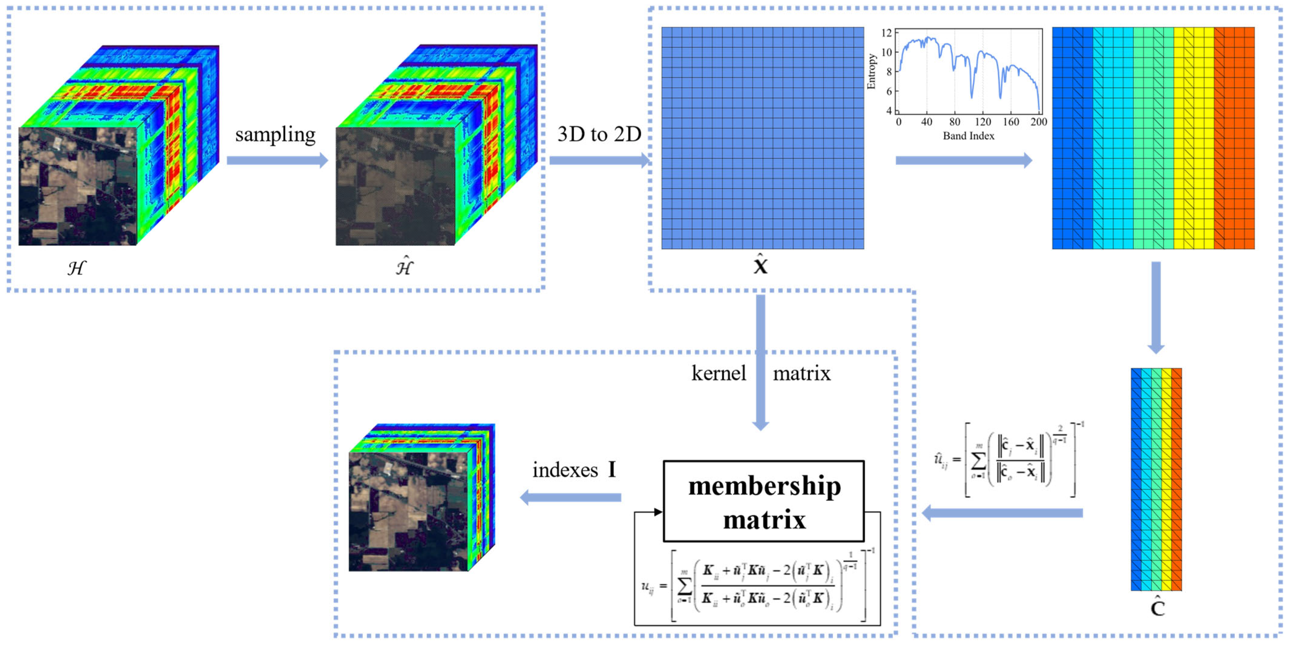
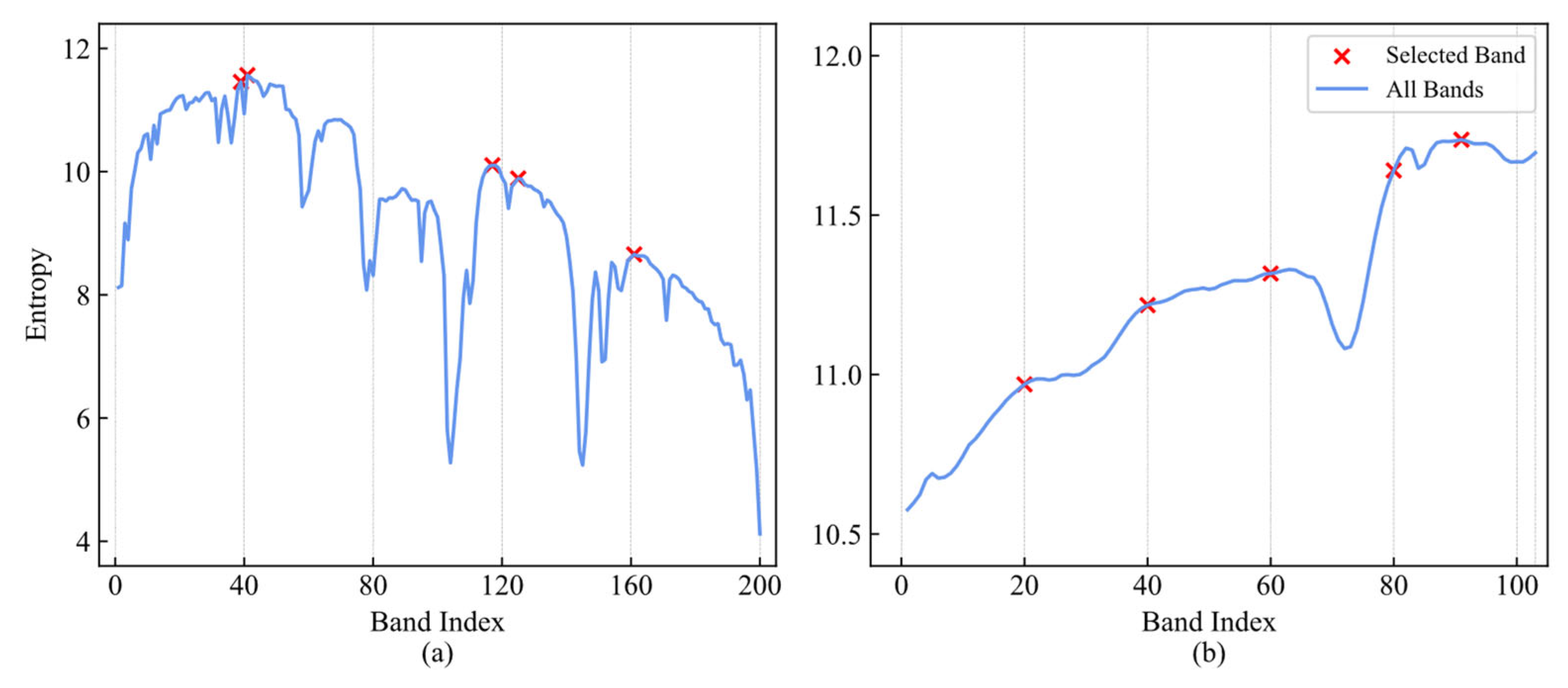
According to the calculation results of information entropy and the number of bands needed, the bands with the highest rank of information entropy are selected as the initial centers of clustering, which can obtain the promising effect of band selection. However, bands with high information entropy may be concentrated in a specific range for HSI, resulting in the selected bands being continuous and not representing the global information of the spectrum well, as shown in Figure 3. Therefore, we propose a grouping information entropy strategy. Specifically, we divide the band information entropy into m groups according to the number of selected bands, then obtain the index value based on the band with the highest information entropy in each group and select the corresponding band vector as the initial cluster center. The method in [48] also uses the concept of grouping, and in the first step of coarse grouping, for the cases that cannot be grouped evenly, the range of the jth group band index is $\left[x_{floor\left(\frac{n\times \left(j-1\right)}{m}\right)+1},x_{floor\left(\frac{n\times j}{m}\right)}\right]$ and $\left[x_{floor\left(\frac{n\times \left(j-1\right)}{m}\right)+1},x_n\right]$ when j < m and j = m, respectively, where floor(∙) denotes rounding down. We remark that our approach is significantly different from [48], as the selection of the grouping strategy to obtain clustering centers is only an initial step in our method. This is to avoid the problem of clustering center aggregation caused by the index sorted using global information entropy. The core of our method lies in the KFCM, not in the grouping strategy. Even if a random grouping operation is employed, the desired results can still be achieved under certain circumstances. However, considering the procedure’s convenience when calculating, this paper chooses even grouping. For bands that are not evenly grouped, the last part is discarded so that the selected bands can be evenly grouped, so the band number in each group is $floor\left(\frac{n}{m}\right)$. As shown in Figure 3, the red marks are the 5 selected bands. We specify that ie_i = H(x_i), the information entropy set of all bands is IE = {ie₁, ie₂, …, ie_n}, and GIE_j represents the set of information entropy of the jth group. The subscript i of ie_i within the grouping still adopts the global index. Since we need to obtain the global index of the band, rather than its position within each grouping, it can be expressed as:

$$\mathbf{I}=\mathit{max} {\mathit{index}}_{j=1}^m({\mathbf{GIE}}_j)$$

(13)

Equation (13) indicates that the subscripts of the maximum values in the m sets or vectors are obtained and formed into sets, and I represents the selected band indices.

Figure 3. Information entropy for each band on two datasets is divided into five groups. (a) Indian Pines; (b) Pavia University.

Figure 3. Information entropy for each band on two datasets is divided into five groups. (a) Indian Pines; (b) Pavia University.

Based on the above process, the proposed SSGIE-KFCM algorithm adopts linear kernel function, spatial cross sampling, and grouping information entropy strategies for band selection. The detailed procedure is shown in Algorithm 1.

Algorithm 1: Procedure of SSGIE-KFCM

Inputs:  HSI data $H\in {ℝ}^{a\times b\times n}$, the number of selected bands m, the weighted index q, the tolerance ε, the number of iterations T.  Output:  The selected band index I. 1  Generate the sampled data $\widehat{H}$ from data $H$ using Equation (11); 2  Convert three-dimensional cube $\widehat{H}$ to two-dimensional matrix $\widehat{\mathbf{X}}$. 3  Calculate the kernel matrix $\widehat{\mathbf{K}}$ of data $\widehat{\mathbf{X}}$ using the linear kernel function $k\left({\widehat{\mathbf{x}}}_i,{\widehat{\mathbf{x}}}_j\right)={\widehat{\mathbf{x}}}_i^{\mathrm{T}}{\widehat{\mathbf{x}}}_j$; 4  Calculate the information entropy of each band using Equation (12); 5  Divide all bands into m groups; 6  Obtain the band index I0 with the highest information entropy in each group according to Equation (13); 7  Select the band according to index I0 as the initial cluster center to form the cluster center matrix $\widehat{\mathbf{C}}$; 8  Calculate the membership matrix $\widehat{\mathbf{U}}$ using Equation (4) and satisfy the constraints in Equation (1); 9  while$\max \left|{\widehat{\mathbf{U}}}^{\left(t+1\right)}-{\widehat{\mathbf{U}}}^{\left(t\right)}\right|<\epsilon$ or T < t do 10  Update the membership matrix $\widehat{\mathbf{U}}$ using Equation (7). 11  end 12  Obtain the band index I of the final $\widehat{\mathbf{U}}$ according to Equation (13); 13  Return I;

4. Experimental Results and Analysis

This section demonstrates the superiority and effectiveness of the proposed SSGIE-KFCM method in various aspects by comparing the experimental classification results of two benchmark HSI datasets. First, the basic details of the two datasets are introduced. Second, we describe the comparison methods and parameter settings. Then, the implementation details and results of classification experiments are discussed and analyzed. In addition, the effects of different spatial sampling strategies on the band selection results are compared. Meanwhile, the effects of information entropy and kernel function techniques on the FCM method are analyzed. Finally, the computational times of different methods are compared, and the advantages of sampling strategy and kernel function in reducing time complexity are verified.

4.1. Experimental Datasets

4.1.1. Indian Pines

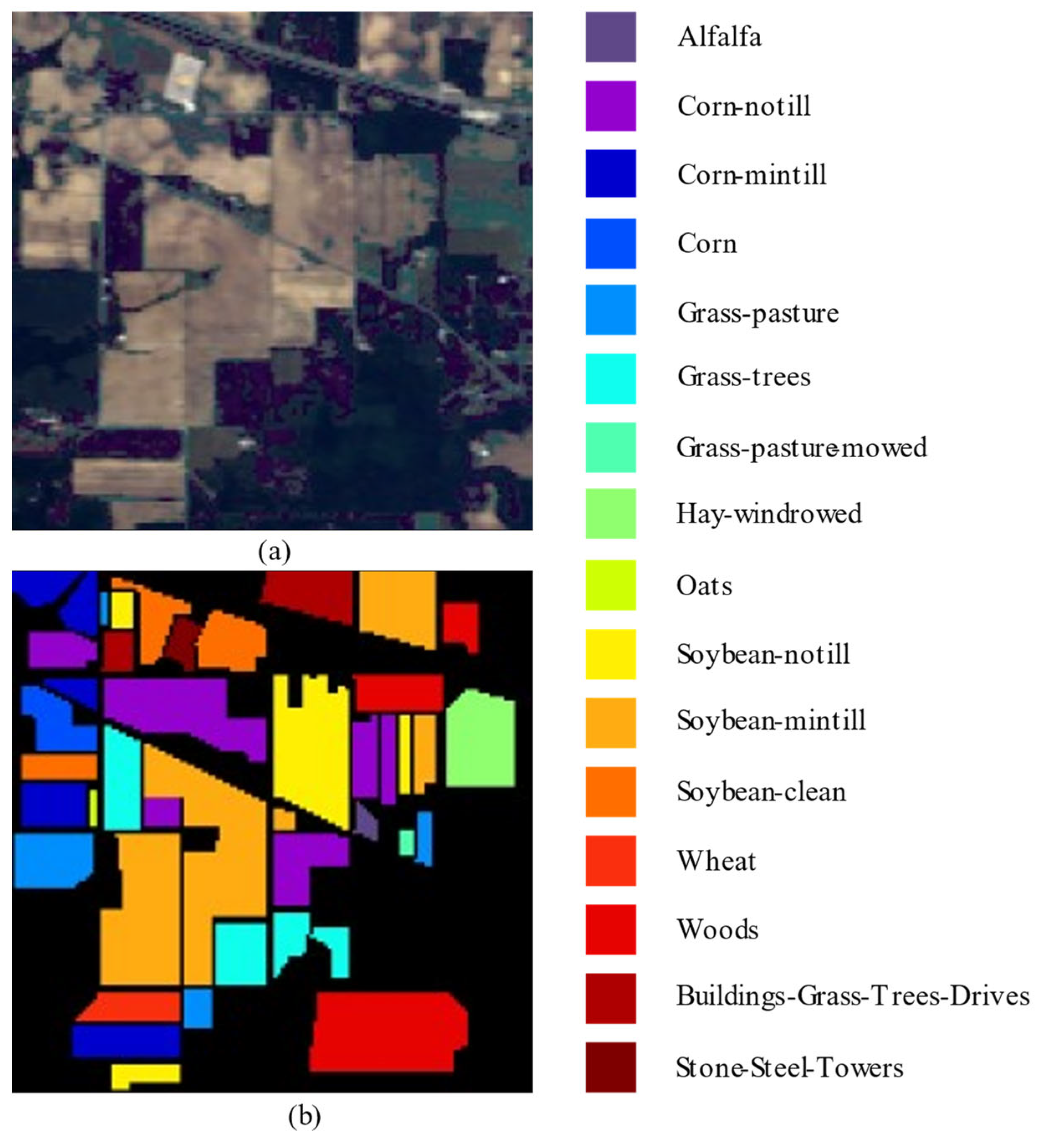
The Indian Pines dataset was collected in 1992 by an AVIRIS sensor at the Indian agriculture and forestry experimental farm in northwest Indiana. It consists of 145 × 145 pixels with 224 spectral bands ranging from 0.4 to 2.5 μm, and its spatial resolution is 20 m. After removing the bands (104–108, 150–163, and 220) that cover the water absorption area, the number of remaining bands is reduced to 200. The actual objects can be classified into 16 categories. This scene is displayed in Figure 4.

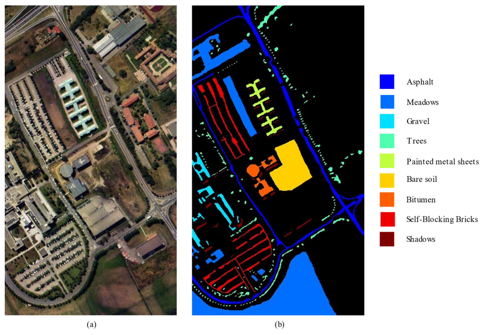
4.1.2. Pavia University

The Pavia University dataset was captured from the ROSIS sensor in the city of Pavia, northern Italy, in 2003, and it contains 610 × 340 pixels and 115 spectral bands varying from 0.43 to 0.86 μm, with a spatial resolution of 1.3 m. Because of the noise band removal, the number of bands used is 103. There are nine categories of ground objects. Figure 5 shows the pseudo-color image and ground object type image of this dataset.

4.2. Comparison Methods and Experimental Settings

To illustrate the effectiveness of the proposed SSGIE-KFCM method, six comparison methods were adopted, including: (1) sparse-based methods: improved sparse subspace clustering (ISSC) [35] and sparse band selection (SpaBS) [33]; (2) ranking-based methods: maximum variance principal component analysis (MVPCA) [40] and ranking-based efficient graph convolution self-representation (EGCSR-R) [49]; (3) a clustering-based method: clustering-based efficient convolution self-representation (EGCSR-C) [49]; and (4) a search-based method: orthogonal projection band selection (OPBS) [50]. The classification results of all bands are added for comparison. The scalar regularization parameter of ISSC is set to 0.001. The sparsity level of SpaBS is 0.05. The numbers of neighbors of EGCSR-R and EGCSR-C are set to 10. The FCM algorithm can obtain the result after 30 iterations according to [31], so we set the number of iterations of SSGIE-KFCM to 50, and the error judgment uses the difference of membership matrix U. The tolerance ε and the weighted index q are set to 0.0001 and 2, respectively.

4.3. Performance Comparison

Support vector machine (SVM) [51] and K-nearest neighbor (KNN) [52] are selected as classifiers to evaluate the effect of band selection. The radial basis function (RBF) is adopted as the kernel function of the SVM classifier, and the penalty coefficient C and the kernel function coefficient gamma are determined by cross-validation with an error accuracy of 0.001. The number of neighbors for the KNN classifier is 3, and the distance measure is Euclidean distance. We randomly selected 20% of the pixels of each class as training samples. In addition, the classification results are primarily evaluated using the overall accuracy (OA), average accuracy (AA), and Kappa coefficients, which are defined as

$$\mathrm{OA}=\frac{1}{N}{\displaystyle \sum _{i=1}^r{y}_{\mathit{ii}}}$$

(14)

$$\mathrm{AA}=\frac{1}{r}{\displaystyle \sum _{i=1}^r\frac{y_{\mathit{ii}}}{y_{i+}}}$$

(15)

$$\mathrm{Kappa}=\frac{N{\displaystyle {\sum }_{i=1}^r{y}_{\mathit{ii}}}-{\displaystyle {\sum }_{i=1}^r\left(y_{i+}\times y_{+i}\right)}}{N^2-{\displaystyle {\sum }_{i=1}^r\left(y_{i+}\times y_{+i}\right)}}$$

(16)

where N and r denote the total number of sample pixels and sample types, respectively. y_ii represents the value in the ith column and the ith row of the confusion matrix, y_i+ is the sum of the elements in the ith row of the confusion matrix, and y_+i is the sum of the elements in the ith column of the confusion matrix.

The number of bands selected for the Indian Pines dataset ranges from 4 to 40, with a step length of 4. For the Pavia University dataset, the number of bands selected is 3 to 30, and the step size is 3. An average of 10 independent experiments was used as the final result.

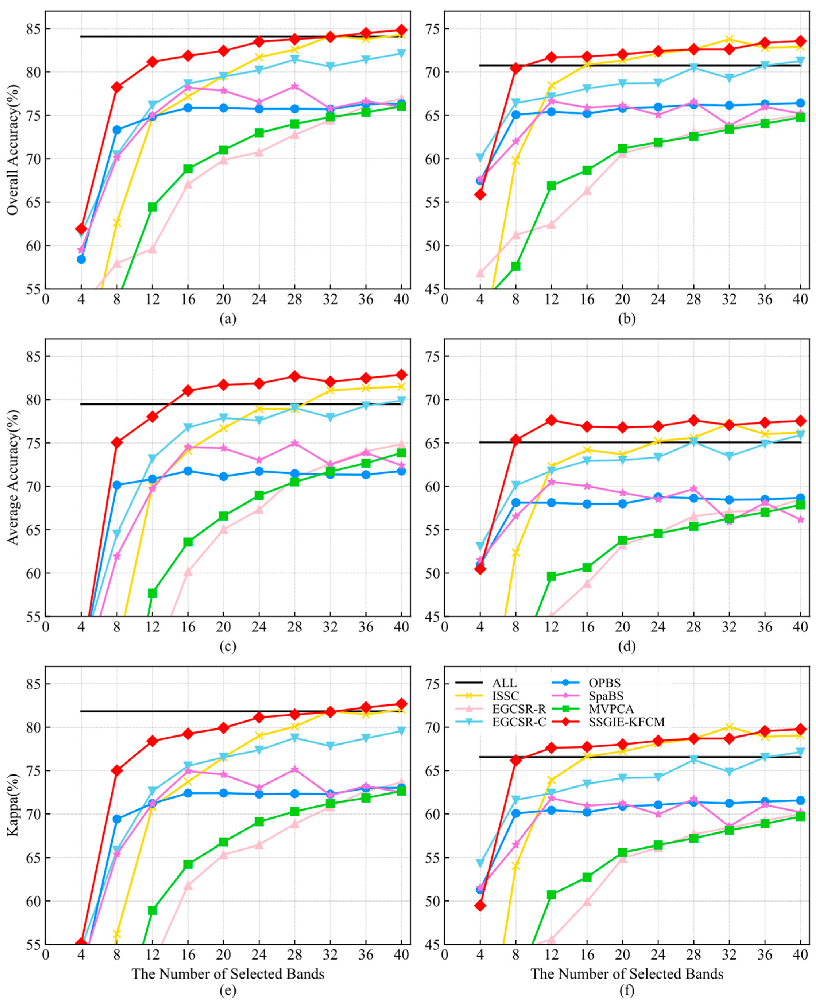
Figure 6 describes the classification accuracy of seven comparison methods using two classifiers on the Indian Pines dataset with different band subset sizes. For the SVM classifier, our proposed SSGIE-KFCM method obtains OA and Kappa values slightly lower than ISSC using 32 selected bands, an AA value slightly lower than EGCSR-C using 4 selected bands, and the classification accuracy of other band subset sizes is the first. More specifically, the performance of SSGIE-KFCM has apparent advantages over other algorithms when selecting the number of bands [8,28]. The OA and Kappa values obtained using 28 bands are similar to those of all bands, and significantly exceed the classification accuracy of all bands at 36 and 40 bands. When the number of selected bands exceeds 16, this achieves an AA value significantly higher than that of the whole band, reaching the maximum when using 40 bands and exceeding the result of 3.39% for all bands. ISSC can also achieve OA and Kappa values using all bands when selecting 32 and 40 bands, and exceed the AA value of the full band at 32, 36, and 40 bands. When using the KNN classifier, the classification accuracy of SSGIE-KFCM is lower than EGCSR-C, OPBS, and SpaBS at 4 bands, slightly lower than ISSC at 32 bands, and the performance corresponding to the other number of bands is the first, which has obvious advantages compared with other methods. The classification accuracy of SSGIE-KFCM can exceed that of all bands when selecting more than eight bands. OA and Kappa values are the highest at 40 bands, exceeding 2.80% and 3.21% of the results using full bands, and the curve of AA reaches the highest at 12 bands, and is 2.54% higher than that of all bands.

Throughout these curves, OPBS achieves a more remarkable classification effect when using four and eight bands, but then it stabilizes without a significant improvement. The accuracy curve of SpaBS is not stable. Although EGCSR-C can continuously improve the accuracy as the number of bands increases, a certain gap in the accuracy exists compared with the proposed SSGIE-KFCM. The performance of EGCSR-R and MVPCA is similar and has also been improving, but poor results have been achieved.

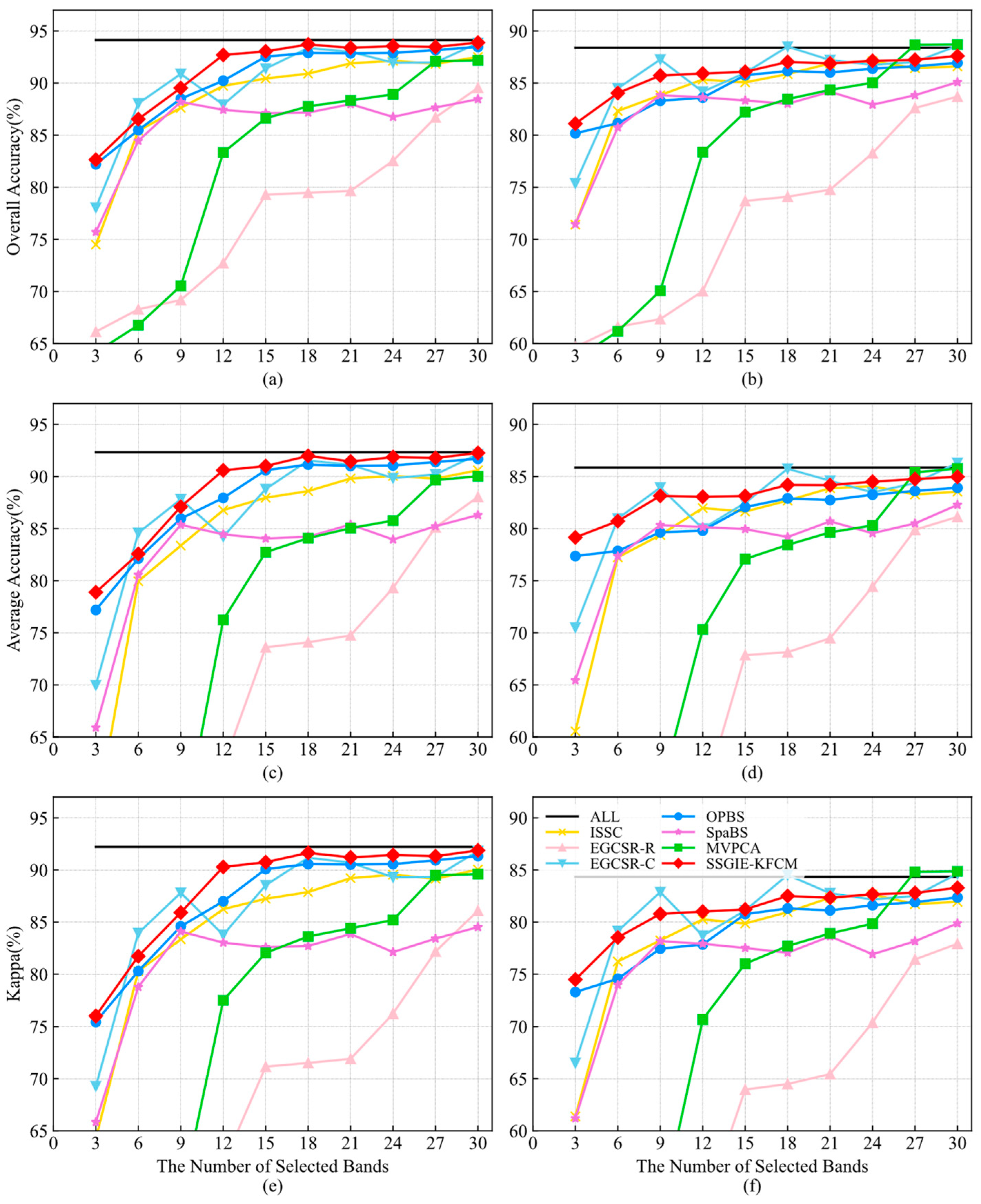
Figure 7 shows the classification accuracy obtained by different band selection methods on the Pavia University dataset. For the SVM classifier, the effect of SSGIE-KFCM is lower than that of EGCSR-C only when six and nine bands are selected, and the effect of the other band subset size is the first. Furthermore, when using 18 bands, it achieves performance close to all bands and remains so. For the KNN classifier, SSGIE-KFCM obtains an accuracy lower than EGCSR-C at 6, 9, 18, 21, and 30 bands, lower than MVPCA at 27 and 30 bands, and the accuracy is first at 3, 12, 15, and 24 bands. However, the accuracy curve of EGCSR-C has a large fluctuation, and the effect of MVPCA is still low when the number of bands selected is small. The ISSC method that performed well on the Indian Pines dataset showed a decrease in performance on the Pavia University dataset, and the overall trend was lower than SSGIE-KFCM, OPBS, and EGCSR-C. OPBS performs better on this dataset than the Indian Pines dataset and is close to our proposed algorithm. Although the performance of MVPCA increases significantly with the number of bands when the number of bands is less than 12, and it can approach or exceed the accuracy of all bands at 27 and 30 bands, the overall results are unsatisfactory, just like the SpaBS and EGCSR-R methods.

From the above analysis, we can see that, in most cases, our proposed SSGIE-KFCM method can obtain the best classification performance, while it is not the best in a few cases. Nevertheless, it can also rank second and third with little difference from the first. When a few bands are selected, the effect of using all bands is achieved. Moreover, for the Indian Pines dataset, the classification accuracy obtained after selecting a certain number of bands is significantly better than that obtained by using all bands, effectively attaining the goal of dimensionality reduction.

4.4. Ablation Study and Sensitivity Analysis

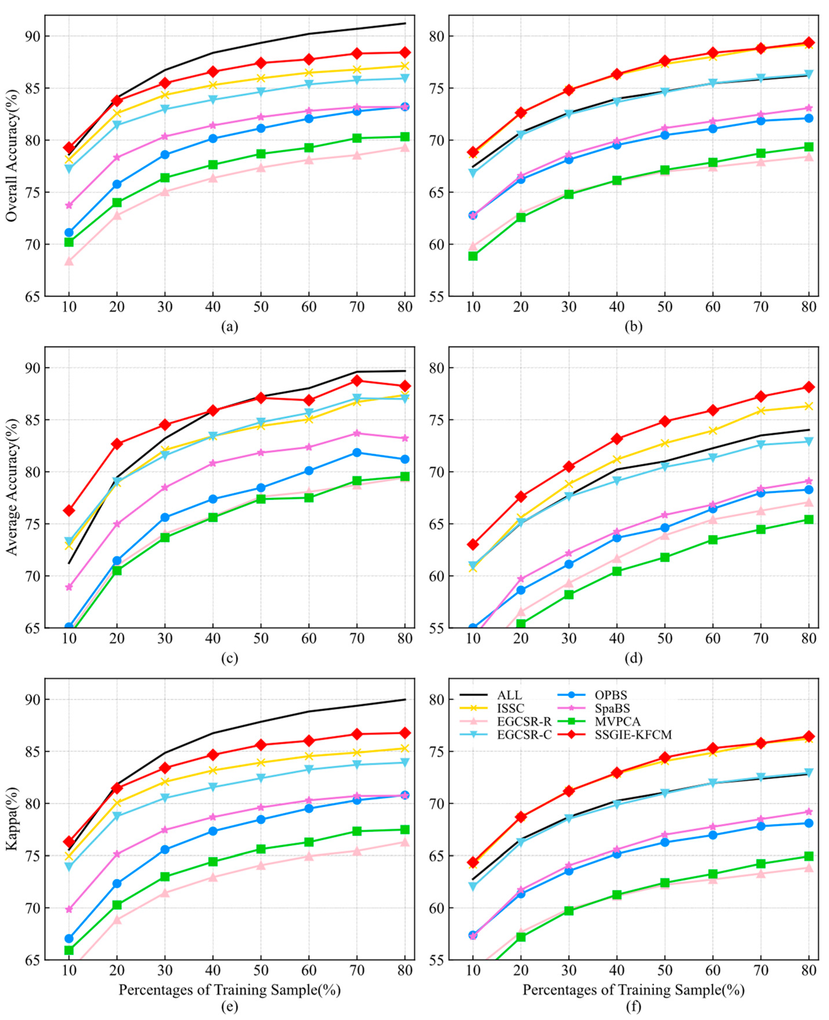
4.4.1. Analysis of Different Training Sample Sizes

This section applies different band selection methods to extract the same number of bands to analyze the relationship between different training sample sizes and band selection results. It then uses the results to implement classification experiments under different classifiers and different proportions of the training sample, in which 10% to 80% of training samples are selected, and the step length is 10%. The experimental results in Section 4.3 show that the classification accuracy of SVM is higher than that of KNN. For the SVM classifier, when the band subset sizes are set to 28 and 18 for the Indian Pines dataset and the Pavia University dataset, the classification performance obtained by some methods is closer to that obtained by using all bands, and can obtain local optimal accuracy. Therefore, this section adopts the number of bands mentioned above for the classification experiments, and the classifier settings and evaluation indices are the same as those in Section 4.3.

Figure 8 indicates the classification accuracy of two classifiers with different training sample sizes using 28 bands given by different methods using the Indian Pines dataset. As you can see from these curves, the proposed SSGIE-KFCM only obtains a slightly lower OA and Kappa of KNN than ISSC using 30% training samples, and the rest are first. For the KNN classifier, it can exceed the OA, AA, and Kappa values of all bands by up to 3.15%, 4.12%, and 3.62%, respectively. The classification accuracy of ISSC is also higher than that of all bands and is almost the same as the OA and Kappa of SSGIE-KFCM. When the proportion of training samples exceeds 50%, EGCSR-C achieves a slightly higher performance than all bands.

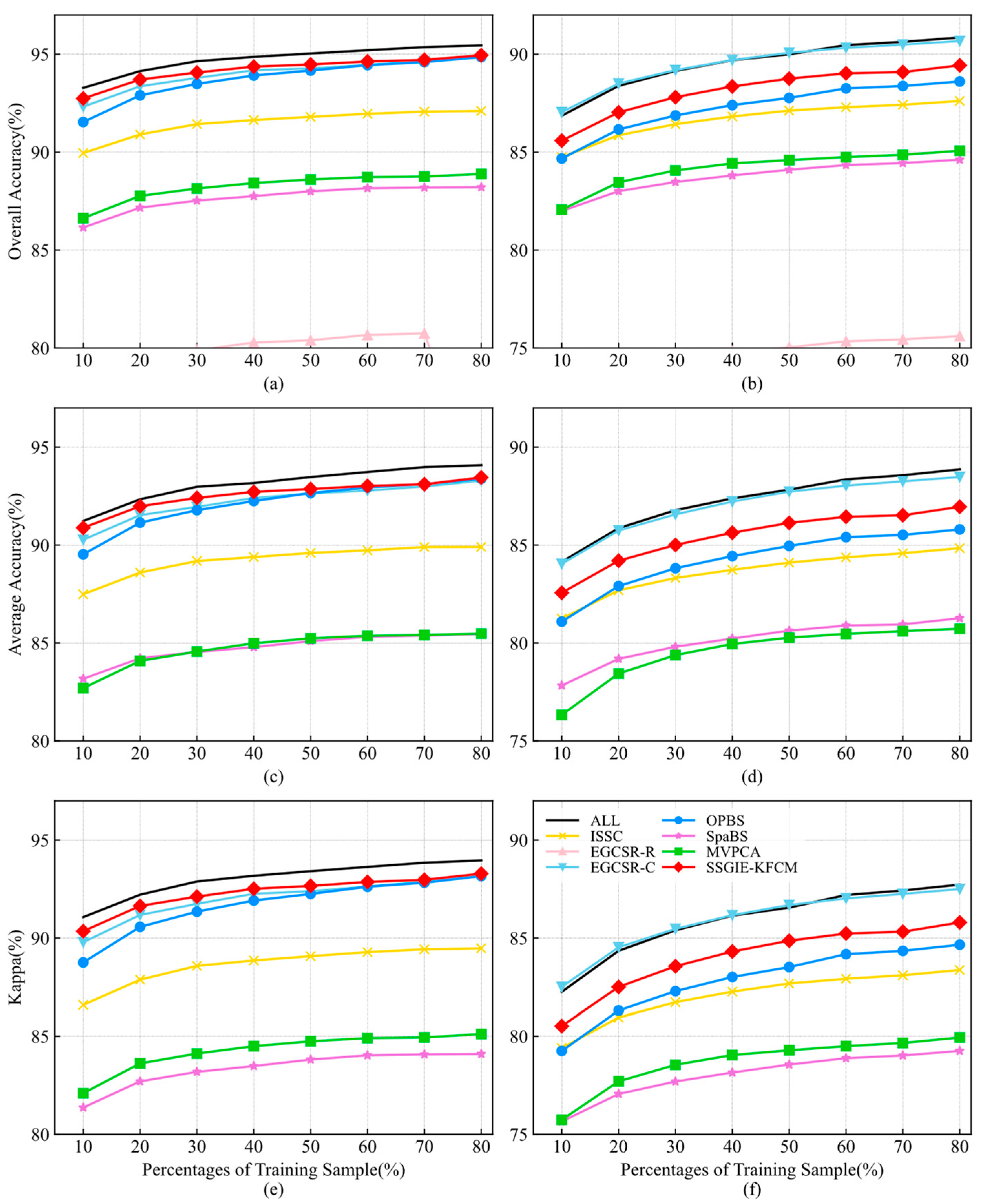
Figure 9 illustrates the classification results using different training sample sizes when 18 bands are selected on the Pavia University dataset. For the SVM classifier, the classification accuracy of SSGIE-KFCM is slightly lower than that of OPBS when 70% of the training samples are used, and the remaining cases are better than the other methods. SSGIE-KFCM, EGCSR-C, and OPBS have a similar performance when the proportion of training samples is from 50% to 80%. For the KNN classifier, SSGIE-KFCM ranks second only after EGCSR-C. SpaBS and MVPCA have similar accuracy and poor results compared with other methods. Due to its low performance, the EGCSR-R method is not within the range of values on the AA and Kappa curves.

As shown in Figure 8 and Figure 9, the classification accuracy increases with the increase in training sample size, but the ranking of band selection methods has no apparent change. The proposed SSGIE-KFCM method is robust to the number of training samples for classification.

4.4.2. Analysis of Different Spatial Sampling Strategies

To analyze and compare the effects of different spatial sampling strategies on band selection results, we performed band selection and classification experiments under different sampling modes, such as non-sampling, row sampling, column sampling, and cross sampling.

Table 1. Classification results of using different sampling strategies on the Indian Pines dataset.

Classifier	Metric	Sampling Strategy	4	8	12	16	20	24	28	32	36	40
SVM	OA	non	61.92	78.24	78.94	81.86	82.44	83.49	83.95	84.03	84.43	84.84
		row	61.92	78.24	81.17	82.01	82.44	83.78	83.95	84.03	84.41	84.74
		col	61.92	78.24	81.17	81.70	82.44	83.78	83.76	84.03	84.48	84.84
		cross	61.92	78.24	81.17	81.86	82.44	83.49	83.77	84.03	84.48	84.84
	AA	non	49.48	75.05	75.92	81.03	81.70	81.85	82.34	82.05	82.41	82.86
		row	49.48	75.05	78.02	80.54	81.70	81.96	82.34	82.05	82.33	82.72
		col	49.48	75.05	78.02	80.16	81.70	81.96	82.24	82.05	82.46	82.86
		cross	49.48	75.05	78.02	81.03	81.70	81.85	82.67	82.05	82.46	82.86
	Kappa	non	55.12	75.00	75.83	79.24	79.91	81.13	81.66	81.75	82.22	82.69
		row	55.12	75.00	78.40	79.40	79.91	81.46	81.66	81.75	82.20	82.58
		col	55.12	75.00	78.40	79.04	79.91	81.46	81.45	81.75	82.29	82.69
		cross	55.12	75.00	78.40	79.24	79.91	81.13	81.46	81.75	82.29	82.69
KNN	OA	non	55.87	70.41	71.28	71.77	72.04	72.40	72.95	72.62	73.37	73.55
		row	55.87	70.41	71.69	71.76	72.04	72.65	72.95	72.62	73.20	73.42
		col	55.87	70.41	71.69	71.45	72.04	72.65	72.94	72.62	73.38	73.55
		cross	55.87	70.41	71.69	71.77	72.04	72.40	72.63	72.62	73.38	73.55
	AA	non	50.48	65.35	67.32	66.88	66.79	66.92	68.09	67.07	67.34	67.54
		row	50.48	65.35	67.61	65.95	66.79	67.20	68.09	67.07	67.22	67.48
		col	50.48	65.35	67.61	65.70	66.79	67.20	68.10	67.07	67.35	67.54
		cross	50.48	65.35	67.61	66.88	66.79	66.92	67.60	67.07	67.35	67.54
	Kappa	non	49.47	66.16	67.15	67.72	68.02	68.43	69.07	68.70	69.55	69.76
		row	49.47	66.16	67.61	67.69	68.02	68.73	69.07	68.70	69.36	69.61
		col	49.47	66.16	67.61	67.34	68.02	68.73	69.05	68.70	69.56	69.76
		cross	49.47	66.16	67.61	67.72	68.02	68.43	68.69	68.70	69.56	69.76

shows the classification results of our method using different sampling strategies on the Indian Pines dataset. The highest values have been marked in bold letters (the same below), and the same accuracy means that the bands selected are the same. It can be seen that when the number of bands selected is 4, 8, 20, and 32, the band indices are identical. For other cases, when 12 bands are used in the SVM classifier, the 3 sampling strategies are 2.23%, 2.10%, and 2.57% higher than OA, AA, and Kappa of the non-sampling operation. Moreover, most of the remaining differences are less than 1%.

The classification results on the Pavia University dataset are listed in

Table 2. Classification results of using different sampling strategies on the Pavia University dataset.

Classifier	Metric	Sampling Strategy	4	8	12	16	20	24	28	32	36	40
SVM	OA	non	61.92	78.24	78.94	81.86	82.44	83.49	83.95	84.03	84.43	84.84
		row	61.92	78.24	81.17	82.01	82.44	83.78	83.95	84.03	84.41	84.74
		col	61.92	78.24	81.17	81.70	82.44	83.78	83.76	84.03	84.48	84.84
		cross	61.92	78.24	81.17	81.86	82.44	83.49	83.77	84.03	84.48	84.84
	AA	non	49.48	75.05	75.92	81.03	81.70	81.85	82.34	82.05	82.41	82.86
		row	49.48	75.05	78.02	80.54	81.70	81.96	82.34	82.05	82.33	82.72
		col	49.48	75.05	78.02	80.16	81.70	81.96	82.24	82.05	82.46	82.86
		cross	49.48	75.05	78.02	81.03	81.70	81.85	82.67	82.05	82.46	82.86
	Kappa	non	55.12	75.00	75.83	79.24	79.91	81.13	81.66	81.75	82.22	82.69
		row	55.12	75.00	78.40	79.40	79.91	81.46	81.66	81.75	82.20	82.58
		col	55.12	75.00	78.40	79.04	79.91	81.46	81.45	81.75	82.29	82.69
		cross	55.12	75.00	78.40	79.24	79.91	81.13	81.46	81.75	82.29	82.69
KNN	OA	non	55.87	70.41	71.28	71.77	72.04	72.40	72.95	72.62	73.37	73.55
		row	55.87	70.41	71.69	71.76	72.04	72.65	72.95	72.62	73.20	73.42
		col	55.87	70.41	71.69	71.45	72.04	72.65	72.94	72.62	73.38	73.55
		cross	55.87	70.41	71.69	71.77	72.04	72.40	72.63	72.62	73.38	73.55
	AA	non	50.48	65.35	67.32	66.88	66.79	66.92	68.09	67.07	67.34	67.54
		row	50.48	65.35	67.61	65.95	66.79	67.20	68.09	67.07	67.22	67.48
		col	50.48	65.35	67.61	65.70	66.79	67.20	68.10	67.07	67.35	67.54
		cross	50.48	65.35	67.61	66.88	66.79	66.92	67.60	67.07	67.35	67.54
	Kappa	non	49.47	66.16	67.15	67.72	68.02	68.43	69.07	68.70	69.55	69.76
		row	49.47	66.16	67.61	67.69	68.02	68.73	69.07	68.70	69.36	69.61
		col	49.47	66.16	67.61	67.34	68.02	68.73	69.05	68.70	69.56	69.76
		cross	49.47	66.16	67.61	67.72	68.02	68.43	68.69	68.70	69.56	69.76

. The results are the same when using non-sampling, row sampling, and column sampling strategies in three bands and non-sampling, row sampling, and cross sampling strategies in six bands. The most significant difference is that when 12 bands are used in the SVM classifier, the cross-sampling strategy results in 1.98%, 1.97%, and 2.72% higher values than the OA, AA, and Kappa values of the non-sampling strategy, and the rest also barely exceed 1%.

The above analysis of the results shows that the use of the spatial sampling strategy will not cause a greater performance loss than non-sampling, or even improve the accuracy. There is no apparent superiority or difference between the three sampling strategies. For the datasets, the Indian Pines scene is more straightforward where any ground object takes up a larger area, and sampling does not have a significant impact on spatial distribution. Hence, it is more likely to select the same band using non-sampling or any sampling strategy than Pavia University.

4.4.3. Analysis of the Grouping Strategy

To compare the effect of different grouping strategies on the classification accuracy of selected bands, we have analyzed the results of truncation grouping in this paper, even grouping in [44], and random grouping strategies for selecting bands. We reiterate that the same precision means the same band is selected. From

Table 3. Classification results of using different grouping strategies on the Indian Pines dataset.

Classifier	Evaluation Indicators	Grouping Strategy	4	8	12	16	20	24	28	32	36	40
SVM	OA	truncate	61.92	78.24	81.17	81.86	82.44	83.49	83.77	84.03	84.48	84.84
		even	61.92	78.24	81.17	82.50	82.44	83.33	83.57	83.24	84.09	84.84
		random	61.92	78.18	79.77	81.80	82.24	82.88	82.99	83.50	83.24	83.64
	AA	truncate	49.48	75.05	78.02	81.03	81.70	81.85	82.67	82.05	82.46	82.86
		even	49.48	75.05	78.02	80.02	81.70	81.56	82.34	80.28	81.95	82.86
		random	49.48	75.28	77.37	79.89	80.14	80.23	81.14	81.23	80.76	81.26
	Kappa	truncate	55.12	75.00	78.40	79.24	79.91	81.13	81.46	81.75	82.29	82.69
		even	55.12	75.00	78.40	79.96	79.91	80.95	81.23	80.85	81.83	82.69
		random	55.12	74.91	76.81	79.17	79.68	80.43	80.56	81.15	80.86	81.32
KNN	OA	truncate	55.87	70.41	71.69	71.77	72.04	72.40	72.63	72.62	73.38	73.55
		even	55.87	70.41	71.69	72.95	72.04	72.34	72.50	71.79	72.42	73.55
		random	55.87	69.93	70.77	71.81	71.79	71.76	72.09	72.01	71.83	72.05
	AA	truncate	50.48	65.35	67.61	66.88	66.79	66.92	67.60	67.07	67.35	67.54
		even	50.48	65.35	67.61	66.60	66.79	66.74	67.55	66.02	66.70	67.54
		random	50.48	65.26	65.56	66.05	65.69	65.58	65.82	65.72	66.02	65.73
	Kappa	truncate	49.47	66.16	67.61	67.72	68.02	68.43	68.69	68.70	69.56	69.76
		even	49.47	66.16	67.61	69.07	68.02	68.36	68.55	67.73	68.46	69.76
		random	49.47	65.61	66.58	67.76	67.73	67.70	68.08	67.99	67.79	68.04

, it can be seen that when 4, 8, 20, and 40 bands are selected, the bands can be evenly grouped and the corresponding bands selected are the same. Overall, the truncation strategy is better than the even strategy and the random strategy, but its predominance is not outstanding, and most of the accuracy difference is less than 1%. In

Table 4. Classification results of using different grouping strategies on the Pavia University dataset.

Classifier	Evaluation Indicators	Grouping Strategy	3	6	9	12	15	18	21	24	27	30
SVM	OA	truncate	82.64	86.54	89.53	92.70	93.04	93.71	93.38	93.55	93.47	93.88
		even	82.64	86.54	89.60	92.70	92.96	93.31	93.58	93.76	93.62	93.71
		random	82.64	86.67	89.90	91.93	92.86	92.86	93.60	93.68	93.91	93.90
	AA	truncate	78.89	82.57	87.10	90.60	91.00	91.98	91.45	91.86	91.78	92.26
		even	78.89	82.57	87.11	90.46	91.12	91.44	91.73	92.03	91.96	92.06
		random	78.89	82.57	87.54	89.78	90.83	90.97	91.83	91.93	92.15	92.20
	Kappa	truncate	76.00	81.72	85.91	90.29	90.75	91.64	91.21	91.43	91.32	91.88
		even	76.00	81.72	86.03	90.29	90.64	91.11	91.47	91.71	91.53	91.65
		random	76.00	81.93	86.44	89.23	90.51	90.50	91.49	91.61	91.91	91.90
KNN	OA	truncate	81.11	84.04	85.72	85.92	86.08	87.03	86.89	87.13	87.23	87.60
		even	81.11	84.04	85.65	86.47	86.67	86.32	87.19	87.07	87.41	87.05
		random	81.11	84.17	85.96	85.92	86.29	86.54	87.18	87.29	87.60	87.37
	AA	truncate	79.16	80.72	83.15	83.06	83.13	84.20	84.18	84.51	84.76	84.97
		even	79.16	80.72	82.83	83.58	83.99	83.61	84.45	84.36	84.81	84.32
		random	79.16	80.59	83.42	83.09	83.38	83.76	84.47	84.57	84.99	84.76
	Kappa	truncate	74.48	78.52	80.78	81.01	81.21	82.51	82.34	82.66	82.80	83.29
		even	74.48	78.52	80.66	81.77	82.02	81.55	82.74	82.56	83.03	82.54
		random	74.48	78.70	81.10	81.01	81.50	81.85	82.73	82.87	83.30	82.98

, the result comparison of the three strategies does not highlight the advantages of one strategy over the other two, which is the same as Table 3, with most accuracy differences being less than 1%.

According to the data of these two tables, the band index selected by different grouping strategies has a slight effect on the final result. In addition, selecting a certain number of bands by grouping is only the initialization step of our proposed SSGIE-KFCM method. Subsequently, it is necessary to optimize the selected results using KFCM.

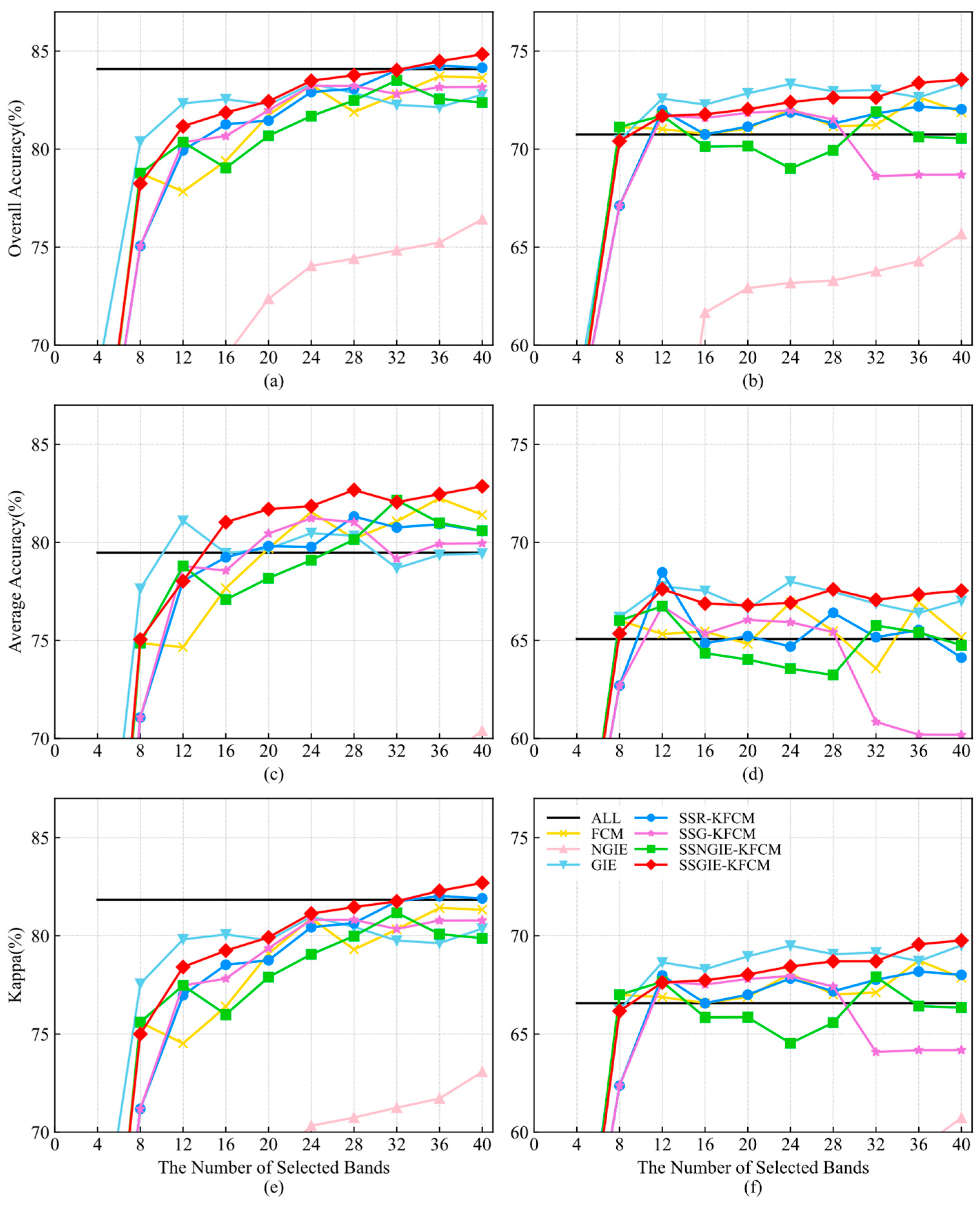
4.4.4. Analysis of Information Entropy and Kernel Function

Ablation experiments are performed to study and analyze the effects of grouping information entropy and kernel functions on the FCM algorithms. All methods are listed in this section, including FCM, no-grouping information entropy (NGIE), grouping information entropy (GIE), kernel FCM using spatial sampling strategy and randomly selected bands as initial cluster centers (SSR-KFCM), kernel FCM using the spatial sampling strategy and grouping selected bands as initial cluster centers (SSG-KFCM), kernel FCM using the spatial sampling strategy and NGIE (SSNGIE-KFCM), and the proposed SSGIE-KFCM. The number of iterations, the tolerance ε and the weighted index q of the FCM are the same as those of SSGIE-KFCM. Figure 10 and Figure 11 describe the ablation results on the two datasets. The GIE uses even grouping in [44].

For the Indian Pines dataset, the FCM method is not stable enough or satisfactory. Furthermore, SSGIE-KFCM has a higher classification performance and stability than FCM. When 12 bands are selected on the SVM classifier, OA, AA and Kappa have the most significant enhancement effects: 3.33%, 3.37% and 3.88%, respectively. SSR-KFCM and SSG-KFCM have almost the same accuracy in OA and Kappa with 4 to 28 bands on both classifiers, but SSG-KFCM has a large drop in the three curves with the KNN classifier and the curve of AA with the SVM classifier at 28 to 32 bands. SSGIE-KFCM has obvious advantages over the two methods, indicating that the bands selected by the grouping information entropy strategy as the initial cluster centers can offer a promising band subset. NGIE achieves a poorer classification result than the other methods because the bands with higher information entropy mentioned in Section 3.4 are concentrated in a particular range, and the selected band range cannot cover the global information. Similar to the performance of MVPCA in Section 4.3, this band selection method, which adopts evaluation criteria to score bands, does not perform well in ranking selected bands in global information. This is also why SSNGIE-KFCM has a poorer result than SSGIE-KFCM, where the initial cluster centers are clustered together. Although GIE achieves a good classification performance on the SVM classifier with fewer bands, it decreases when the three accuracy indices reach their higher positions at 12 bands, tending to stabilize. The classification accuracy of SSGIE-KFCM at 20 bands exceeds that of GIE and increases with the number of bands, gradually exceeding the accuracy of all bands. GIE has higher OA and Kappa values on the KNN classifier than SSGIE-KFCM, but it is not stable on the AA index. This grouping information entropy strategy of grouping first and then selecting representative bands in each group, which is consistent with the idea of clustering methods, can be regarded as a simple clustering method. Compared with NGIE, it proves the superiority of the clustering method over the ranking-based method.

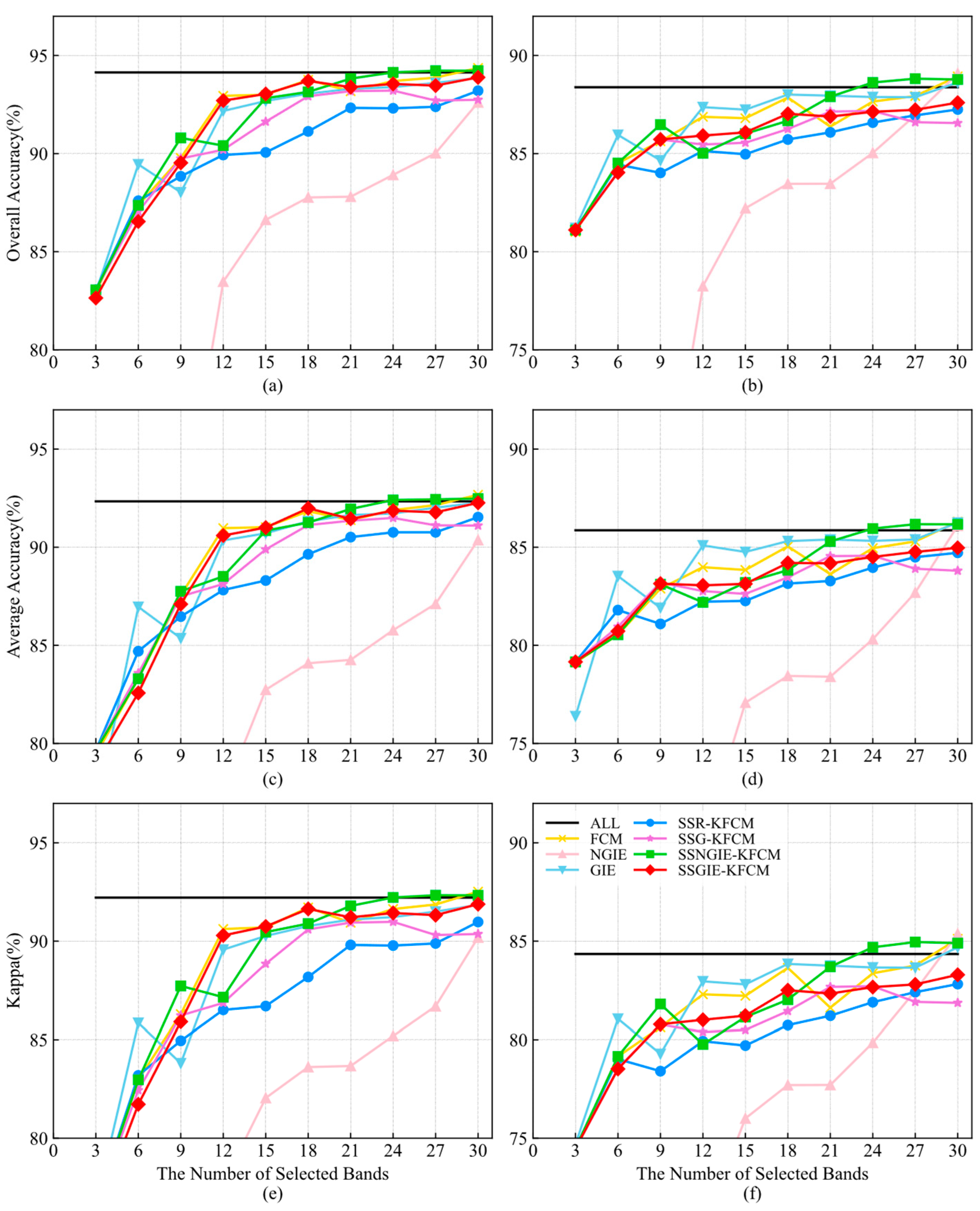
As seen from Figure 11, like the results on the Indian Pines dataset, NGIE has poorer classification results. SSR-KFCM and SSG-KFCM still have some differences from SSGIE-KFCM, but SSG-KFCM has a better performance than SSR-KFCM on this dataset, indicating that these bands cover the global segmented selection and are used as the initial cluster centers to achieve better results. GIE performs better on this dataset than the Indian dataset and has a similar performance to SSGIE-KFCM on the SVM classifier. However, it is superior to SSGIE-KFCM only when 3, 6, and 27 bands are selected, and both classifiers have a significant drop at 9 bands. SSGIE-KFCM works better when there are fewer bands, and SSNGIE-KFCM works better when there are more than 21 bands. For the SVM classifier, FCM has almost the same classification accuracy as SSGIE-KFCM, and FCM has a higher classification accuracy with the KNN classifier.

4.5. Computational Time Complexity Analysis

4.5.1. Comparisons of Computation Times

The running time metric is used to assess the computational complexity of different methods, and the number of bands selected on the Indian Pines and Pavia University datasets is also 28 and 18.

Table 5. Calculational time (in seconds) of different methods.

Dataset	ISSC	EGCSR-R	EGCSR-C	OPBS	SpaBS	MVPCA	SSGIE-KFCM
Indian Pines	9.471	0.125	4.040	4.231	127.130	0.030	0.506
Pavia University	40.635	0.543	2.189	11.221	542.487	0.142	1.066

lists the operating time of seven methods on two datasets. All experiments were based on Python 3.9 and run on the same PC with an Intel i9-10900X CPU with 64-GB RAM to ensure fairness. MVPCA runs the fastest among these methods, with less than 1 s of computing time, followed by EGCSR-R. However, it should be noted that these two methods perform poorly in classification accuracy and are not recommended, even though they have faster running speeds. OPBS and EGCSR-C have similar computation times on the Indian Pines dataset, but EGCSR-C has less running time on the Pavia University dataset. SpaBS takes more time and has a higher cost than the other algorithms. The proposed SSGIE-KFCM method takes less time than MVPCA and EGCSR-R and runs for less than 1 s on the Indian Pines dataset, but it has higher classification accuracy and obvious advantages compared to the latter.

4.5.2. Effectiveness of Sampling Strategy and Kernel Function

This section will analyze the effectiveness of the sampling strategy and the kernel function used in this paper in reducing the computational complexity. Specifically, the computational time of FCM, SSGIE-KFCM and the method without spatial sampling (GIE-KFCM) is counted. To better compare the running time gaps between the three methods, we recorded the calculational time of selecting 10 to 50 bands on the two datasets with a step of 10 and calculated the ratio of FCM and GIE-KFCM to SSGIE-KFCM.

Table 6. Calculational time (in seconds) of different methods.

Dataset	Number of Bands	Computational Times			Time Ratio
		FCM	GIE-KFCM	SSGIE-KFCM	FCM/SSGIE-KFCM	GIE-KFCM/SSGIE-KFCM
Indian Pines	10	7.541	0.408	0.313	24.1	1.3
	20	11.885	0.498	0.370	32.1	1.3
	30	19.700	0.718	0.521	37.8	1.4
	40	23.799	0.859	0.633	37.6	1.4
	50	32.207	0.989	0.673	47.9	1.5
Pavia University	10	85.184	2.016	0.835	102.1	2.4
	20	174.567	3.504	1.146	152.4	3.1
	30	266.661	3.855	1.461	182.5	2.6
	40	348.403	5.773	1.767	197.2	3.3
	50	434.991	5.758	2.072	210.0	2.8

gives the calculational time of selecting different band subset sizes for these methods. It can be seen that the time consumed increases with the number of bands. With the same number of bands, the Pavia University dataset takes longer to compute than the Indian Pines dataset because the Pavia University dataset has a wider spatial range and a larger number of pixels. The introduction of kernel function greatly accelerates the computational efficiency, while the sampling strategy can further shorten the time, making the running time of SSGIE-KFCM the shortest. Compared with FCM, SSGIE-KFCM is at least 24.1 times more efficient for the Indian Pines dataset and 102.1 times more efficient for the Pavia University dataset. On the Pavia University dataset, SSGIE-KFCM has a greater degree of computational complexity reduction than GIE-KFCM, which is also due to the larger spatial scale and the more pronounced effect of sampling strategies.

5. Conclusions

In this paper, we proposed a novel band selection algorithm—SSGIE-KFCM—by applying kernel function, spatial sampling, and a grouping information entropy strategy to the FCM algorithm to address the feature redundancy problem of HSI data. This method optimizes the iterative process of FCM and obtains better initial cluster centers by using grouping information entropy. Then, it reduces the amount of computational data via the spatial sampling strategy and employs the kernel function to improve the execution efficiency. The experimental results on two publicly available datasets indicate that adding the sampling strategy and kernel function effectively improves the computational efficiency of FCM. The more significant the amount of data and the more bands selected, the more pronounced the improvement effect is. Meanwhile, adopting grouping information entropy improves the effect of band selection. Compared with the FCM method, the classification accuracy of OA is improved by 3.33%, AA by 3.37%, and Kappa by 3.88%, at most. The bands selected by the SSGIE-KFCM method can reach or even exceed the classification performance of all bands, and OA is improved by 2.80%, AA by 3.39%, and Kappa by 3.20%, at most, which achieves the purpose of dimensionality reduction.

Compared with other methods, our proposed SSGIE-KFCM obtains better classification accuracy and stability with less running time and is more robust to different classifiers and parameter settings. The linear kernel function utilized in this paper has no parameters. In FCM, the weighted index q is usually 2, the number of iterations is 50, and the tolerance ε is set to 0.001 or 0.0001. Hence, our method does not need to adjust parameters and is more convenient to use than ISSC, EGCSR-R, EGCSR-C, or SpaBS. In a nutshell, the comparison and analysis of the experiments verify that SSGIE-KFCM is competitive.

The proposed SSGIE-KFCM method has achieved remarkable results in improving computational efficiency, but there is still room for improvement in accuracy, which will be our future research content. In addition, this paper only studies the effect of linear kernels. In the future, we will discuss the impact of different kernels on this method and the reasons.