Impact of Drought on Isoprene Fluxes Assessed Using Field Data, Satellite-Based GLEAM Soil Moisture and HCHO Observations from OMI

Abstract

Biogenic volatile organic compounds (BVOCs), primarily emitted by terrestrial vegetation, are highly reactive and have large effects on the oxidizing potential of the troposphere, air quality and climate. In terms of global emissions, isoprene is the most important BVOC. Droughts bring about changes in the surface emission of biogenic hydrocarbons mainly because plants suffer water stress. Past studies report that the current parameterization in the state-of-the-art Model of Emissions of Gases and Aerosols from Nature (MEGAN) v2.1, which is a function of the soil water content and the permanent wilting point, fails at representing the strong reduction in isoprene emissions observed in field measurements conducted during a severe drought. Since the current algorithm was originally developed based on potted plants, in this study, we update the parameterization in the light of recent ecosystem-scale measurements of isoprene conducted during natural droughts in the central U.S. at the Missouri Ozarks AmeriFlux (MOFLUX) site. The updated parameterization results in stronger reductions in isoprene emissions. Evaluation using satellite formaldehyde (HCHO), a proxy for BVOC emissions, and a chemical-transport model, shows that the adjusted parameterization provides a better agreement between the modelled and observed HCHO temporal variability at local and regional scales in 2011–2012, even if it worsens the model agreement in a global, long-term evaluation. We discuss the limitations of the current parameterization, a function of highly uncertain soil properties such as porosity.

1. Introduction

Biogenic volatile organic compounds (BVOCs) are highly reactive and have large effects on the oxidizing potential of the troposphere, air quality and climate [1,2,3]. They are mainly emitted by terrestrial vegetation and amount to ca. 1000 Tg year⁻¹ globally, with about half of the share consisting of one compound, isoprene [4,5,6,7,8]. Isoprene influences tropospheric hydroxyl radical levels through multiple processes [9,10,11,12,13,14], thereby altering the lifetime of methane. Under high-NO_x conditions, it is a major precursor of tropospheric ozone [2,15,16,17,18] and it also affects the growth of secondary organic aerosols [19,20,21,22], both of which are considered as important short-lived climate forcers.

Extreme events such as droughts bring about changes in the surface emissions of biogenic hydrocarbons. Under mild to moderate drought, water stress can either have no significant impact on isoprene emission or can stimulate it, even in case of a significant inhibition of photosynthesis (e.g., [23,24,25]). In fact, there is evidence that isoprene improves plant thermotolerance [26,27,28]. This increase in isoprene emissions has been hypothesized as a possible result of the drought-induced stomatal closure, which causes a reduction in transpiration rates as the plants attempt to conserve water, and subsequently increases leaf temperature [29,30]. However, as water stress becomes more severe, the general consensus is that isoprene emission capacity of a plant is greatly reduced [23,24,25,30,31,32].

The effects of drought stress on isoprene emissions have been investigated in several studies, most of which were conducted in the laboratory [33,34,35,36,37,38]. Field observations at ecosystem-scale during natural droughts are scarce [30,32,39,40] and, to the authors’ knowledge, only one site provides measurements of isoprene fluxes. During the 2011–2012 field campaigns in central U.S., at the Missouri Ozarks AmeriFlux (MOFLUX) site, isoprene and other BVOC fluxes were monitored for two consecutive growing seasons concomitant to two drought events [30,32]. Moreover, the effect of drought on isoprene may also be monitored at greater spatiotemporal scales using other proxies. Formaldehyde (HCHO) is a key intermediate in the oxidation of the large majority of hydrocarbons released by vegetation, anthropogenic activities and fire. BVOCs, among which isoprene is largely dominant, are the major precursors of HCHO over vegetated areas (e.g., [41,42,43]), and therefore, satellite HCHO is an excellent proxy for the emissions of BVOCs. The anthropogenic signal of HCHO is low and only detectable in highly polluted regions [44,45], and does not play a role in the isoprene-dominated MOFLUX site area. The contribution of fires to the HCHO abundances is generally important in the vicinity of fires or downwind, but only small agricultural fires occurred during the summers of 2011 and 2012 over Missouri. The BVOC emissions are therefore the main driver of the HCHO interannual variability over Eastern US [46]. Zheng et al. (2017) [47] have shown that remotely sensed sun-induced fluorescence (SIF) and HCHO columns qualitatively capture reductions in flux-derived gross primary productivity (GPP) and isoprene emission at the MOFLUX site, respectively, on weekly to monthly time scales, but with muted responses. They concluded that even fairly moderate reductions in satellite SIF and HCHO column could be indicative of severe soil drought.

The present study aims at assessing the response of isoprene emissions to drought modelled by the Model of Emissions of Gases and Aerosols from Nature (MEGAN; [5,48]). The current parameterization in MEGANv2.1, dependent on root-zone soil water content and permanent wilting point (denoted ${\theta }_W$), was derived based on a study conducted on potted plants [33]. It was found unable to account for the response of isoprene emissions to the severe drought during the 2012 MOFLUX campaign, and the low value of ${\theta }_W$ assumed for the site was designated the main culprit [32]. In addition to errors in the formulation and ${\theta }_W$, uncertainties have been pointed out in relation to the MEGANv2.1 drought parameterization. The reduction in global annual isoprene emissions entailed by this drought factor ranges between 7 and 50% for different model configurations [6,48,49,50,51]. The range is even wider (10–70%) when varying the soil moisture input datasets ([52,53]). In addition, MEGAN is typically run using reanalysis data, and thus does not benefit from the four-decades of progress in the field of microwave surface soil moisture retrievals [54].

The objective of this study is to update the drought parameterization in MEGANv2.1 [5] using (i) the 2011–2012 MOFLUX field measurements, and (ii) remotely sensing-based root-zone soil moisture from the Global Land Evaporation Amsterdam Model (GLEAM; [55,56]). GLEAM assimilates surface soil moisture retrievals from the ESA Climate Change Initiative soil moisture (ESA CCI SM; [57]) into a multilayer soil model driven by observation-based precipitation. GLEAM soil moisture recently proved to outperform the reanalysis estimates used in MEGAN in comparison to in situ measurements [58]. The influence on isoprene emissions of the updated MEGAN parameterization using GLEAM data is evaluated at different scales using the models (biogenic emission and chemistry-transport) and observations (in situ and remotely sensed) described in Section 2. The assessment of the re-adjusted algorithm at the site-, regional- and global-scales is presented in Section 3, with the regional study performed over the contiguous U.S. for 2011–2012. The evaluation method used here is based on spaceborne HCHO and a chemistry-transport model, and relies on the high HCHO yield from the oxidation of isoprene. This method has been widely used in past studies [42,43,59,60,61,62]. Discussion and conclusions are drawn in Section 4.

2. Materials and Methods

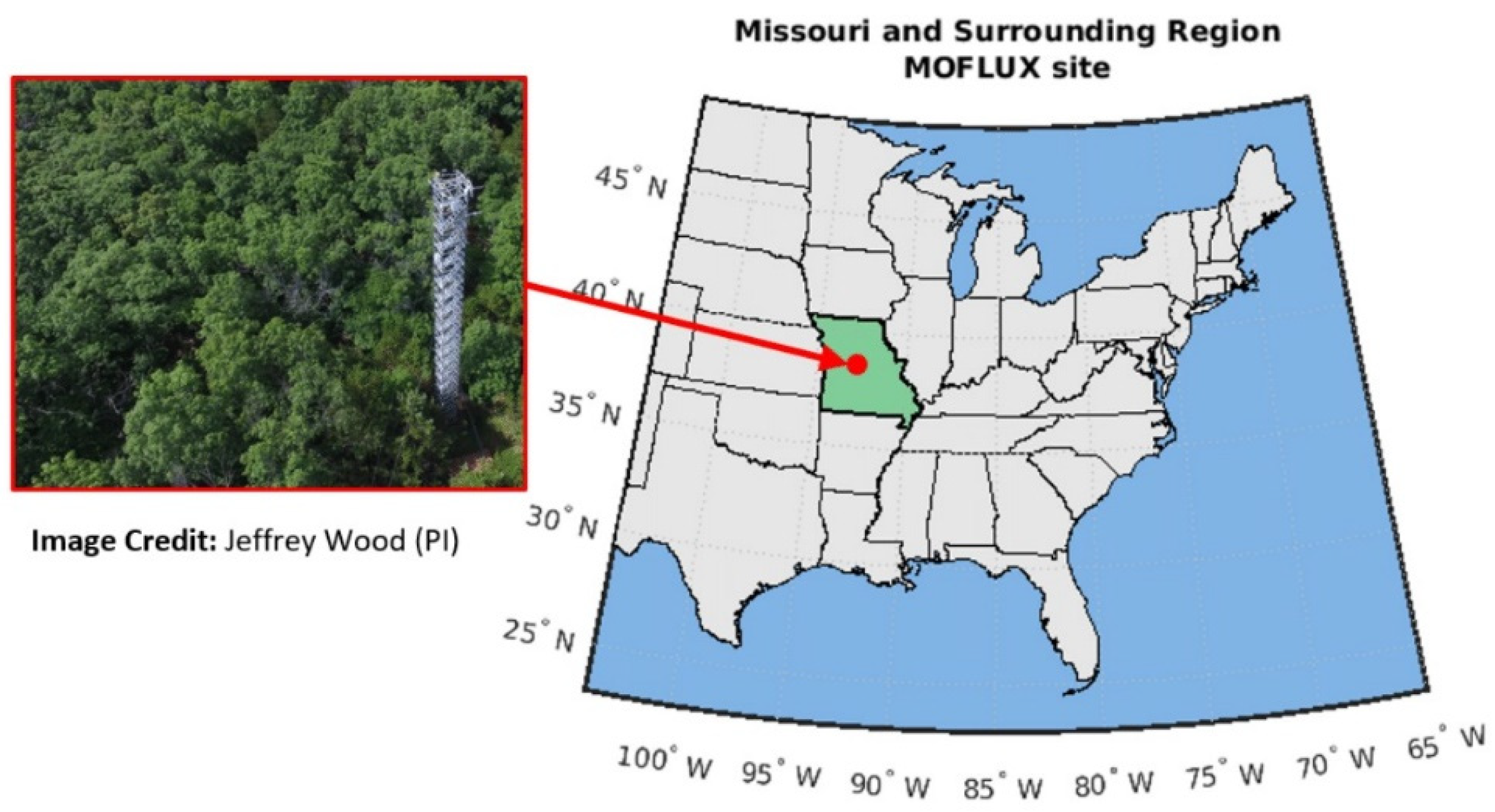
2.1. Site Description and Eddy-Covariance Flux Measurements

The MOFLUX field site is located in central U.S., in the Ozarks region of Missouri state (38°44.65′N latitude, 92°12.00′W longitude, 219 m elevation; Figure 1). It is part of the AmeriFlux network and has provided continuous eddy covariance measurements of carbon dioxide, water and energy fluxes since 2004. The 32-m tower is surrounded by a continuous broadleaf deciduous forest within a 1-km radius. The tower extends about 10 m above the top of the canopy. The forest is oak dominated, with two thirds of the trees belonging to white and red oak species, and the remaining third being hickory, sugar maple, ash, and juniper. With this abundance of isoprene-emitting species of oaks, the Ozarks area has gained the nickname of ‘isoprene-volcano’, holding the record for the highest isoprene fluxes ever reported (53.3 mg m⁻² h⁻¹) during the 2011 campaign [30]. The relatively thin silt loam soils prevent the trees from reaching deep soil moisture during droughts, which exacerbates plant water stress [63]. Soil water retention curves ([64]) for the Weller silt loam soils near the MOFLUX eddy covariance tower indicate a wilting point of 0.13 m³ m⁻³ for the top 0–30 cm soil depth, and 0.23 m³ m⁻³ for soil depths below 30 cm. These figures correspond to the water content at −1.5 MPa soil matric potential, a value that commonly defines ${\theta }_W$ [65].

The area is classified as a humid subtropical climate in the Köppen classification and is prone to droughts between July and September [66,67]. In 2011 and 2012, the site has respectively suffered from mild and severe droughts for which two campaigns of VOC flux measurements were conducted. [30] used a chemiluminescence analyzer for the 2011 campaign spanning from 18 May to 2 September. The dataset is provided with a half-hour frequency. The 2012 campaign of [32] was extended to other compounds than isoprene. Eddy covariance fluxes were calculated half-hourly with a proton transfer reaction quadrupole mass spectrometer (PTR-Quad-MS) and covered a nearly six–months period from 2 May to 22 October. According to the U.S. Drought Monitor, the most intense period of drought occurred in August 2012 with exceptional drought conditions (i.e., level D4) affecting more than a third of Missouri land (https://www.drought.gov/states/missouri, accessed on 23 June 2021).

2.2. MEGAN-MOHYCAN: Biogenic VOC Emission Modelling

The biogenic emissions of isoprene, monoterpenes, and 2-methylbutenol are estimated using MEGAN [5,48] coupled to the MOdel for HYdrocarbon emissions by the CANopy (MOHYCAN; [49,68]), a multi-layer canopy environment model. The net emission rates F (µg m⁻² h⁻¹) into the above-canopy atmosphere are estimated as follows:

$$F=\mathsf{\epsilon }\cdot {\gamma }_0, with {\gamma }_0=C_{CE}\cdot {\gamma }_{PT}\cdot LAI\cdot {\gamma }_A\cdot {\gamma }_{SM}\cdot {\gamma }_{C{O}_2},$$

(1)

where the emission factor ε (µg m⁻² h⁻¹) represents the emission rate at standard conditions as defined by [48]. Deviations from those conditions are accounted for by the activity factors encapsulated in ${\gamma }_0$ representing the response of biogenic emissions to their major identified environmental and phenological drivers. Activity factors account for leaf temperature and photosynthetic photon flux density (${\gamma }_{PT}$), leaf area index (LAI), leaf age (${\gamma }_A$), drought stress (${\gamma }_{SM}$) and CO₂ inhibition (${\gamma }_{C{O}_2}$). The temperature and light response algorithm incorporates the influence of current and past conditions, as well as the attenuation of light by leaves within the canopy. The calculation of ${\gamma }_{PT}$ is performed by MOHYCAN, the canopy environment model, detailed by [49]. The adjustment factor C_CE is specific for each canopy environment model and is set to 0.52 for MOHYCAN, so that ${\gamma }_0=1$ for standard canopy conditions. The response of biogenic isoprene emissions to drought in the MEGAN model is accounted for primarily in the ${\gamma }_{SM}$ activity factor through the direct impact of soil water stress on the emissions. Moreover, drought leads to enhanced stomatal resistances and therefore higher leaf temperatures accounted for in ${\gamma }_{PT}$ defined in MOHYCAN. For severe drought conditions, however, the impact of ${\gamma }_{SM}$ outweighs the impact of higher leaf temperatures, and can even lead to a complete shutdown of the emissions [33].

Currently, the MEGAN model provides the users with two algorithms of ${\gamma }_{SM}$ for the response of emissions to drought. In MEGANv2.1, the impact of drought is estimated based on the volumetric soil water content (denoted $\theta$) and ${\theta }_W$. The factor ${\gamma }_{SM}$ accounts for direct deviations due to changes in $\theta$ as follows:

$${\gamma }_{SM}=\{\begin{array}{cc}1& \theta >{\theta }_1\\ \frac{\theta -{\theta }_W}{\Delta \theta }& {\theta }_{W }<\theta <{\theta }_1\\ 0& \theta <{\theta }_W\end{array}$$

(2)

The original value of $\Delta \theta$ (0.06 m³ m⁻³; [48]) was derived empirically based on the study of [33] conducted on potted plants, with one plant species (Populus deltoides Bartr.) and soil type. The value $\Delta \theta$ was later lowered to a more conservative 0.04 m³ m⁻³ [5], because emissions were being shut off in regions where there was no extreme drought, and will further be referred to as the default value for this parameter. The threshold point ${\theta }_1$ is defined as ${\theta }_W+\Delta \theta$. As emphasized by [49], the soil water content should be paired consistently with the wilting point given the importance of the wilting point in the determination of soil moisture.

In the third version of the model (MEGANv3; [69]), isoprene emissions respond simultaneously to water stress and photosynthesis, as provided by the Community Land Model (CLM; [70]) in the Community Earth System Model (CESM; [71]), which is coupled to MEGAN. The parameterization of the drought stress activity factor ${\gamma }_{SM}$ in MEGANv3 (hereafter denoted ${\gamma }_{SM}^{\ast }$) is based on CLM maximum rate of carboxylation ($V_{CMAX}$) and soil moisture stress function (${\beta }_t$). A thorough description of these parameters is provided in [70] and the parameterization is fully discussed in [69]. The estimation of ${\gamma }_{SM}^{\ast }$ follows:

$${\gamma }_{SM}^{\ast }=\{\begin{array}{cc}\hfill 1& {\beta }_t>0.6\\ \hfill V_{CMAX}/\alpha & 0<{\beta }_t<0.6\\ \hfill 0& {\beta }_t=0\end{array}$$

(3)

The empirical parameter α (=37) was calibrated by [69] based on field measurements at the MOFLUX site.

Two evaluation approaches are considered to assess the response of biogenic isoprene emissions to drought in the MEGAN biogenic emission model. Single-point estimations of isoprene fluxes using algorithms from Equations (2) and (3) are evaluated against measurements conducted in 2011 and 2012 presented hereinabove. Global and regional (over North America) approaches are also conducted through the assessment of tropospheric HCHO columns using satellite-based observations against simulations from a chemistry transport model that accounts for ${\gamma }_{SM}$ (Equation (2)) with different values of $\Delta \theta$.

The MEGAN-MOHYCAN model is set up for the MOFLUX site as follows. Single-point model simulations of daily isoprene fluxes for years 2011 and 2012 are performed using local meteorological conditions provided by the AmeriFlux website (https://ameriflux.lbl.gov/sites/siteinfo/US-MOz, accessed on 23 June 2021). Hourly measurements of air temperature and photosynthetic photon flux density from the tower are used. Daily LAI measurements for the 2012 campaign were obtained from [32]. Since direct local measurements of LAI were not available to us for 2011, we use the daily 2012 values, corrected for interannual variation based on monthly averaged Moderate Resolution Imaging Spectroradiometer (MODIS) LAI (MODIS 15A2H collection 6 available at https://lpdaac.usgs.gov, accessed on 15 June 2021) at 0.5° resolution in the vicinity of the MOFLUX site. More precisely, the 2012 local values are multiplied by the ratio of MODIS LAI between the two years (Figure S1). The canopy emission factor ε was set to 8.6 mg m⁻² h⁻¹. The value is chosen such that the model without any drought stress correction (${\gamma }_{SM}=1$) matches the average measured isoprene fluxes of the 2011 campaign, when the effect of drought was of lesser magnitude. As will be seen in Section 3, the ${\gamma }_{SM}$ parameterization has an almost negligible impact in 2011.

In the following, the simulation without stress (${\gamma }_{SM}=1$) will be referred to as the baseline. The impact of drought stress is accounted for by multiplying the baseline emissions by either daily ${\gamma }_{SM}$ (Equation (2)) or ${\gamma }_{SM}^{\ast }$ (Equation (3)). The latter was obtained using CLM5 (instead of CLM4.5 as in Jiang et al., 2018) and local environmental conditions observed at the MOFLUX site. The daily ${\gamma }_{SM}$ is obtained using daily satellite-based root-zone $\theta$ provided by the GLEAM model at 0.25° × 0.25° spatial resolution, along with the ${\theta }_W$ distribution taken from the static soil properties defined in GLEAM (see Section 2.3). For reasons explained in Section 3.1, the empirical parameter $\Delta \theta$ is re-evaluated and set to $\Delta \theta =0.12$; the adjusted factor using GLEAM is referred to as ${\gamma }_{SM}^{OPT}$. The drought factor using the default $\Delta \theta =0.04$ is denoted ${\gamma }_{SM}^{0.04}$.

2.3. Satellite-Based Soil Properties from GLEAM

GLEAM [55,56] is a set of algorithms to derive the different components of terrestrial evaporation and soil moisture (surface and root-zone) from satellite-based datasets of different hydro-climatic variables at a daily timescale. It employs the Priestley and Taylor equation [72] to estimate potential evaporation for different land cover types (short and tall vegetation, bare soil, ice and snow covers, and open water). A semi-empirical, land cover-dependent multiplicative stress factor is used to translate the potential evaporation estimates into actual evaporation. For tall and short vegetation, the stress factor is based on vegetation optical depth [73] and root-zone soil moisture. For bare soil, the stress factor is dependent on surface soil moisture only. Interception loss is estimated using the Gash analytical model [74]. To model surface and root-zone soil moisture, GLEAM applies a multi-layer soil water balance. The number of soil layers and the depth of the root-zone depend on land-cover type with a maximum depth of 10 cm for bare soil, 100 cm for low vegetation, and 250 cm for tall vegetation, respectively. The soil water available for evaporation, either via transpiration or bare soil evaporation, is estimated using static soil properties (e.g., ${\theta }_W$) taken from the database of Global Gridded Surfaces of Selected Soil Characteristics generated by the International Geosphere-Biosphere Programme Data and Information System (IGBP-DIS, [75]). Finally, GLEAM incorporates a data assimilation module which ingests soil moisture observations via a Newtonian nudging scheme. In the version of GLEAM used in this study (GLEAMv3.5b), the latest satellite-based estimates of surface soil moisture from ESA-CCI [76] are assimilated, which include observations from the Soil Moisture Active Passive (SMAP) satellite. GLEAMv3.5b data at daily and 0.25° × 0.25° resolution are available for download at www.gleam.eu (accessed on 1 April 2022).

2.4. Remotely Sensed Formaldehyde Columns from OMI

We use formaldehyde observations retrieved from the Ozone Monitoring Instrument (OMI) spectrometer aboard the Aura mission launched in 2004 [77]. The OMI HCHO product used in this study was developed in the framework of the EU FP7 project QA4ECV (Quality Assurance for Essential Climate Variables, http://www.qa4ecv.eu, accessed on 1 June 2018) and is fully documented by [78,79]. The retrievals of HCHO slant columns are based on improved Differential Optical Absorption Spectroscopy (DOAS) algorithms that reduce the effect of interferences between species using the 328.5–359 nm spectral window with the HCHO absorption cross-section from [80]. Further, the background normalization of the slant columns is performed using the equatorial Pacific Ocean in order to compensate for possible systematic latitude-dependent offsets in spectral fitting. The conversion into a vertical column is performed with the air mass factor (AMF) obtained by combining an altitude-resolved AMF look-up table derived at 340 nm from the VLIDORTv2.6 radiative transfer model [81] and the daily a priori formaldehyde vertical profile shape calculated with the TM5-MP chemical transport model [82,83]. The scattering due to clouds is corrected using an independent pixel approximation [84], whereas the effects of non-absorbing aerosols are implicitly accounted for through the cloud correction scheme. The effect of absorbing aerosols is currently not accounted for in the retrieval algorithm. Those effects can be significant over regions dominated by biomass burning or over heavily industrialized regions.

The OMI QA4ECV dataset provides separate estimates for the systematic and random components of the total uncertainty and a thorough description of the error estimation is provided in [85]. The total uncertainty on the monthly HCHO vertical column generally ranges between 20% and 40%, depending on the observation conditions. For clear sky conditions, in absence of aerosols, the total error on the AMFs is estimated at 18% and the error increases with cloud fraction, up to 50% for a cloud fraction of 0.5. The omission of the aerosol correction may lead to a significant underestimation of the derived HCHO column by up to 40% over fire scenes [80]. To ensure the best quality, we filter out cloudy pixels (fractions higher than 20%) in addition to the quality assurance criterion (http://www.tropomi.eu/sites/default/files/files/publicSentinel-5P-Formaldehyde-Readme.pdf, accessed on 25 September 2021). This already limits the potential impact of thick plumes on the retrievals. Furthermore, we conducted an additional sensitivity analysis aiming to minimize the potential impact of aerosols on the model comparisons with OMI HCHO data. This was done by filtering out OMI pixels with high aerosol optical depth (AOD), as described in Section 2.6 below and Section S6 of the Supplementary Materials.

For the comparison with MOFLUX data, the OMI observations are averaged within a 20-km radius around the MOFLUX site. For the regional and global evaluation, observations at 0.5° × 0.5° and 2° × 2.5° are used, respectively.

2.5. Simulated HCHO Columns Using MAGRITTE and IMAGES CTMs

Simulations of HCHO columns are performed using the Model of Atmospheric composition at Global and Regional scales using Inversion Techniques for Trace gas Emissions (MAGRITTE) v1.1, a global and regional three-dimensional chemistry-transport model (CTM) of the troposphere [86,87]. Most model parameterizations are inherited from the global Intermediate Model of the Global and Annual Evolution of Species (IMAGESv2) model [46,61,88,89,90]. MAGRITTE calculates the concentrations of 182 chemical compounds in the troposphere with a spin-up time of six months. The horizontal resolution of the model is either 2° (latitude) × 2.5° (longitude) at a global scale or 0.5° × 0.5° at a regional scale, while the vertical coordinate is a hybrid sigma-pressure system resolved in 40 unevenly spaced levels extending from the surface to the lower stratosphere (44 hPa). Meteorological fields are provided by European Centre for Medium-Range Weather Forecasts (ECMWF) ERA-Interim reanalyses. The model calculates monthly averaged columns at the OMI overpass time (13:30), taking into account the sampling date statistics of the satellite. The chemical degradation mechanism of isoprene relies on the Leuven isoprene mechanism [11,91] and the Caltech oxidation mechanism [92], accounting for relevant theoretical and laboratory studies.

The bottom-up fluxes of HCHO precursors are prescribed as follows. The biomass burning inventory is obtained from the Global Fire Emission Database version 4 (GFED4s; [93]) on a daily basis (https://globalfiredata.org, accessed on 22 March 2013). The anthropogenic sources of non-methane VOC species are taken from the Emission Database for Global Atmospheric Research version 4.3.2 (EDGARv4.3.2, [94]) and the anthropogenic CO, NO_x, OC, SO₂, BC and NH₃ are obtained from the Hemispheric Transport of Air Pollution version 2 (HTAPv2; [95]) database for 2010. Due to their limited availability, the EDGARv4.3.2 emissions are set constant at their 2012 values after this year. Both inventories are available at https://edgar.jrc.ec.europa.eu (accessed on 28 August 2018). Over the U.S., the anthropogenic EDGAR emissions are scaled down to match emission estimates based on aircraft NO_x concentrations and nitric acid deposition data, according to [96]. Biogenic emissions are prescribed as follows. As in [46], MEGAN-MOHYCAN global simulations provided fluxes of isoprene, monoterpene, and 2-methyl-3-buten-2-ol (MBO) using meteorological fields from ECMWF reanalysis (ERA-Interim; [97]) and gridded emission factors [5] based on detailed land cover description and species-specific emission factors. The global bottom-up inventory of biogenic isoprene emissions is publicly available from emissions.aeronomie.be/index.php/bottom-up/isoprenev2018 (accessed on 1 April 2022). Biogenic sources of ethylene, formaldehyde, and acetone, based on the MEGAN model are taken from the database of Emissions of atmospheric Compounds and Compilation of Ancillary Data (ECCAD, http://eccad.aeris-data.fr, accessed on 3 June 2019). Biogenic emissions of acetaldehyde and ethanol are parameterized as in [98]. Finally, the biogenic methanol emissions are provided by inverse modelling constrained by spaceborne methanol data [99]. Finally, monthly 3-dimensional methane concentration distributions are prescribed, based on an assimilation of surface data at 0.75° resolution provided by the Copernicus Atmospheric Monitoring System (CAMS) (https://ads.atmosphere.copernicus.eu, accessed on 21 April 2022).

The HCHO column assessment is performed at three different scales: local, regional and global. Regional simulations of formaldehyde columns are conducted using the regional MAGRITTE model at a 0.5° resolution for the U.S. (10–54°N, 65–130°W) for a period of 30 months starting on 1 July 2010 (including the spin-up time). For the local analysis, we extract HCHO columns at the 0.5° grid cell of the regional model including the MOFLUX site. The lateral boundary conditions of the regional model are provided by a global model simulation using the same chemical mechanism and emission datasets. Three model simulations were performed: one simulation without water stress (referred to as MAGRITTE, ${\gamma }_{SM}=1$), and two simulations with the monthly ${\gamma }_{SM}$ factor calculated using Equation (2) with monthly root-zone $\theta$ from GLEAM with different values of the empirical parameter $\Delta \theta$, namely the default value 0.04 (referred to as MAGRITTE, ${\gamma }_{SM}^{0.04}$) and the value of 0.12 obtained from the optimization of the model at the MOFLUX site (referred to as MAGRITTE,${\gamma }_{SM}^{OPT}$). The global, long term comparison relies on the monthly HCHO columns obtained with IMAGES, for which two simulations are performed over the 2005–2016 period at a horizontal resolution of 2° × 2.5°, using either the default value 0.04 (referred to as IMAGES, ${\gamma }_{SM}^{0.04}$) or the value of 0.12 (referred to as IMAGES, ${\gamma }_{SM}^{OPT}$).

2.6. Aerosol Optical Depth Dataset

For our alternative analysis based on OMI data excluding high-AOD pixels, we use gridded, total AOD at 469 nm from the CAMS global reanalysis EAC4 (ECMWF Atmospheric Composition Reanalysis 4; https://ads.atmosphere.copernicus.eu/#!/home, accessed on 22 February 2022). CAMS AOD is constrained by MODIS [100] and the Advanced Along-Track Scanning Radiometer (AATSR; [101]) aboard Envisat from 2003 to March 2012. Moreover, they are routinely evaluated against in situ data such as the AErosol RObotic NETwork (AERONET). A more complete description of the CAMS aerosol scheme can be found in [102].

3. Results

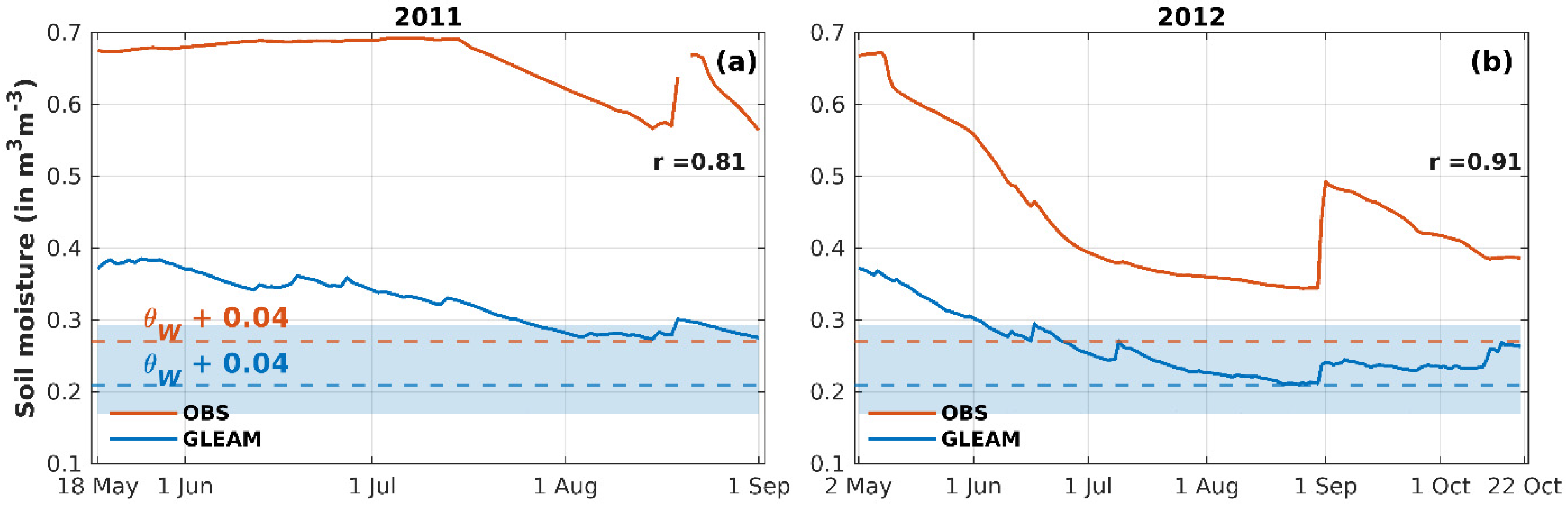
3.1. Soil Water Content and Soil Moisture Stress Factor

The ${\gamma }_{SM}$ factor (Equation (2)) depends explicitly on the plant water status. Figure 2 shows the daily $\theta$ as measured at a depth of 100 cm and as represented by the root-zone (0–250 cm) GLEAM product at the grid cell encompassing the MOFLUX site in years 2011 and 2012. The exceptional conditions of 2012 are shown by the decrease in the observed $\theta$, from 67% at the beginning of May to a minimum of 34% by the end of August. The drought condition was relieved with the return of precipitation illustrated by the sharp increase in the $\theta$ at the end of August 2012. The mild drought of 2011 had a lesser impact on $\theta$, which decreased from 70% in July to 56% in August.

The root-zone $\theta$ of GLEAM correlates well with in situ observations in both years, with Pearson’s coefficients of 0.81 and 0.91. While part of the bias stems from differences in soil depths and spatial horizontal resolution, model biases are expected due the ill-representation of certain soil properties (field capacity, critical and residual soil moisture, etc.); nonetheless, absolute values are expected to differ due to the lack in regional representativeness of soil moisture point in situ measurements, mainly due to the high spatial variability in porosity. The local mean porosity varies between 0.55 m³ m⁻³ at 50 cm and about 0.70 m³ m⁻³ at the surface (Jeffrey D. Wood, personal communication), based on measurements at four locations around the Missouri site; the IGBP-DIS porosity used in GLEAM is 0.43 m³ m⁻³ at the site, and vertically constant.

Following the ${\gamma }_{SM}$ parameterization of MEGANv2.1, both the locally measured $\theta$ (orange line on Figure 2) and the GLEAM $\theta$ (blue line) always exceed the default threshold value, ${\theta }_1$ = ${\theta }_W$+ 0.04, represented by dashed lines in Figure 2. The threshold is estimated at 0.27 m³ m⁻³ based on local ${\theta }_W$, and at 0.21 m³ m⁻³ in GLEAM based on the IGBP-DIS ${\theta }_W$ value. This implies that the isoprene fluxes are not impacted by the drought stress activity factor (i.e., ${\gamma }_{SM}=1$) according to the MEGANv2.1 parameterization.

Therefore, the current parameterization fails to capture the drought effect due to the low value of the empirical parameter $\Delta \theta$, which was based on only one study [33]. Therefore the $\Delta \theta$ value is re-calibrated using the MOFLUX measurements, in order to derive an optimal value of the parameter $\Delta \theta$ that provides the best match with the MOFLUX isoprene dataset. To that aim, we vary the $\Delta \theta$ parameter in the model and select the value which minimizes the root-mean square error (RMSE) between modelled and in situ daily fluxes in both years. Using the soil moisture and ${\theta }_W$ from GLEAM, the optimized $\Delta \theta$ is 0.12. Using this value, the GLEAM $\theta$ falls below the threshold ${\theta }_1$ of 0.29 (= 0.12 + 0.17) during several weeks in 2011 (after 28 July) and the entire summer and early fall in 2012 (after 5 June).

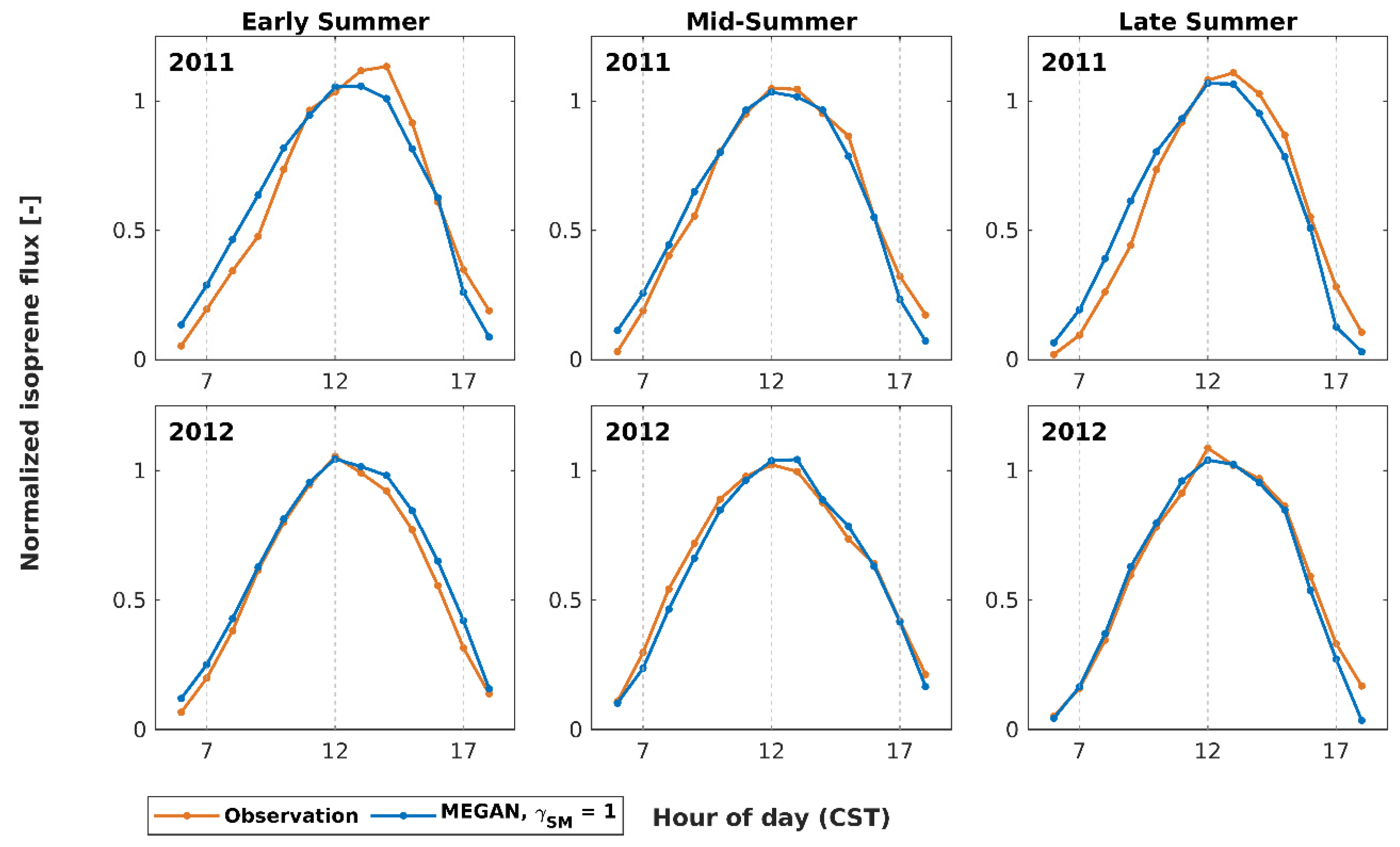
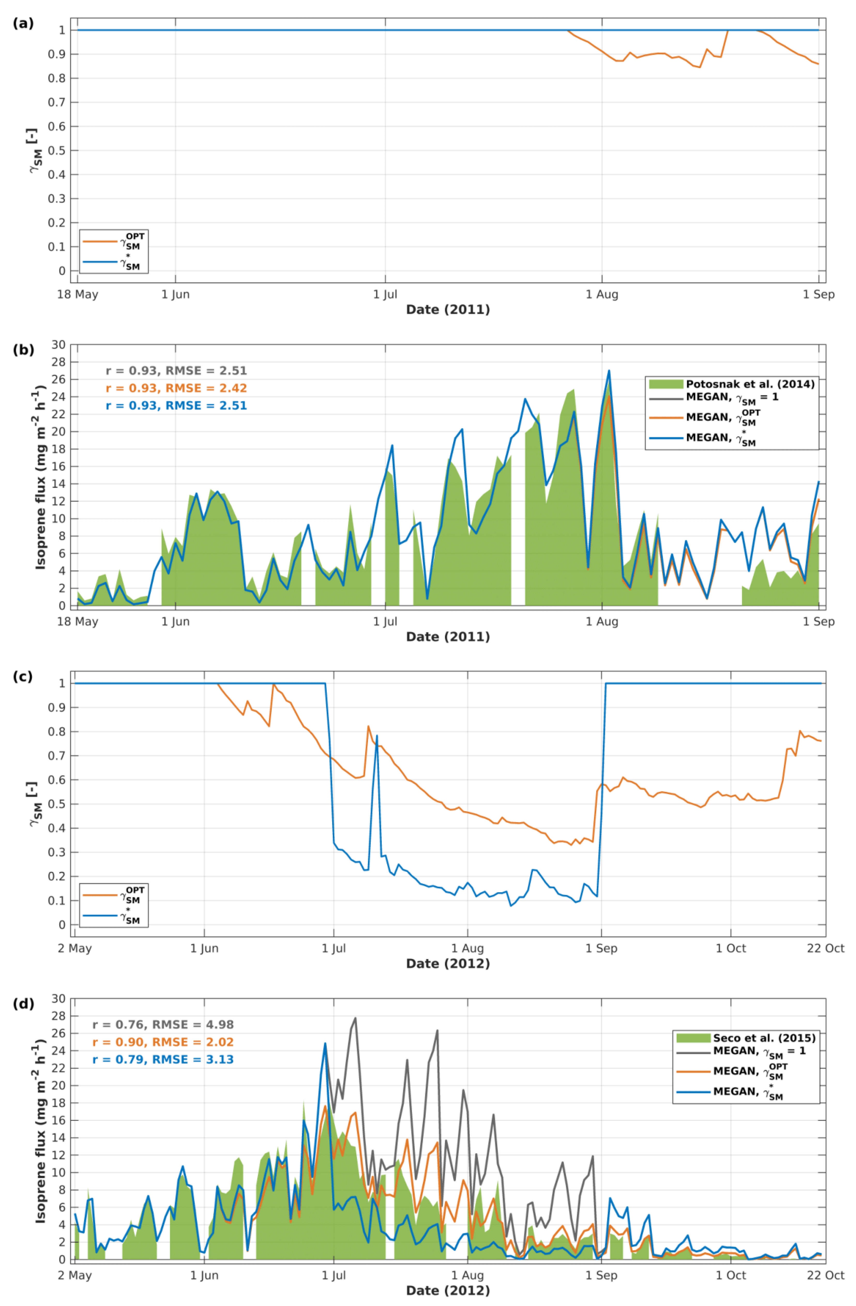
3.2. Daily Time Series and Diel Cycle

During the mild drought year, the daily drought stress factors have virtually no impact on isoprene fluxes except when adopting the optimized factor ${\gamma }_{SM}^{OPT}$, which entails a flux reduction of about 10% during the month of August (Figure 3a). The bias-corrected MEGAN simulations explain 93% of the variability of daily isoprene fluxes during summer 2011 for the simulations using ${\gamma }_{SM}^{OPT}$ or using ${\gamma }_{SM}=1$ (Figure 3b). Measurements are missing during 10–17 August due to an equipment failure. The reasons for the model overestimation in the second half of August are unclear, but could be partly due to an underestimation of the effect of leaf age as previously noted in MEGAN comparisons with flux measurements at a temperate forest [49].

In the severe stress year (2012), the model performance is lowest in the no-stress configuration (${\gamma }_{SM}=1$) both in terms of correlation (r = 0.76) and root-mean square error (RMSE = ~5 mg m⁻² h⁻¹, Figure 3d). The ${\gamma }_{SM}^{\ast }$ factor improves only slightly the comparison (r = 0.79 and RMSE = ~3 mg m⁻² h⁻¹), whereas the application of ${\gamma }_{SM}^{OPT}$ improves the fit in 2012 to r = 0.90 and RMSE = ~2 mg m⁻² h⁻¹. The stress factor ${\gamma }_{SM}^{OPT}$ decreases the isoprene fluxes from early June to late October, with a maximum reduction of about 70% at the end of August, and a significant decrease of 40–50% in late summer (Figure 3c). In the measurement dataset, the highest daily flux occurs on June 24, at ~18 mg m⁻² h⁻¹. Without the stress factor, modelled isoprene fluxes peak 12 days later, on 6 July. Those fluxes overestimate the observations by 6.00 mg m⁻² h⁻¹ in July August (a percentage bias of about 98%). This bias is strongly reduced (to 0.42 mg m⁻² h⁻¹) due to the application of ${\gamma }_{SM}^{OPT}$ i.e., ~7%. The drop in emissions is sharper with ${\gamma }_{SM}^{\ast }$, up to 90% in July August (Figure 3c), leading to a model underestimation reaching 3.13 mg m⁻² h⁻¹ (about −58%) for that same period (Figure 3d). The improvement of estimated isoprene fluxes using ${\gamma }_{SM}^{OPT}$ is also seen in the drop in the RMSE from ~5 mg m⁻² h⁻¹ to roughly 2 mg m⁻² h⁻¹. Overall, the comparison shown in Figure 3 points to a better agreement with the use of ${\gamma }_{SM}^{OPT}$ compared to ${\gamma }_{SM}^{\ast }$. Finally, the model succeeds at reproducing the normalized diel pattern of emission fluxes (Figure 4), independent of the application of the drought stress factor. Nevertheless, the diurnal peak occurs sooner in 2011, by one hour in June, and as much as 2 h in late summer.

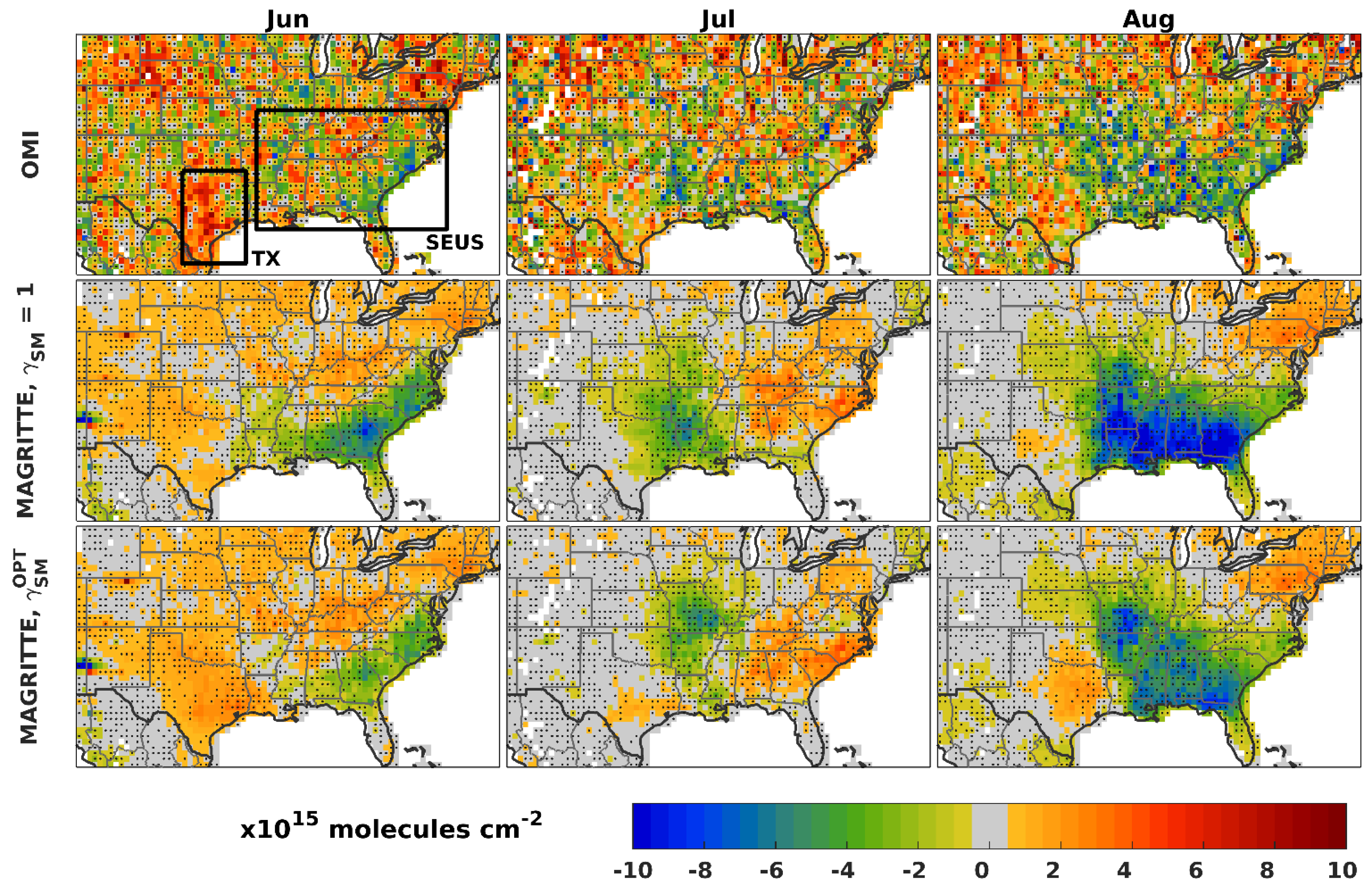
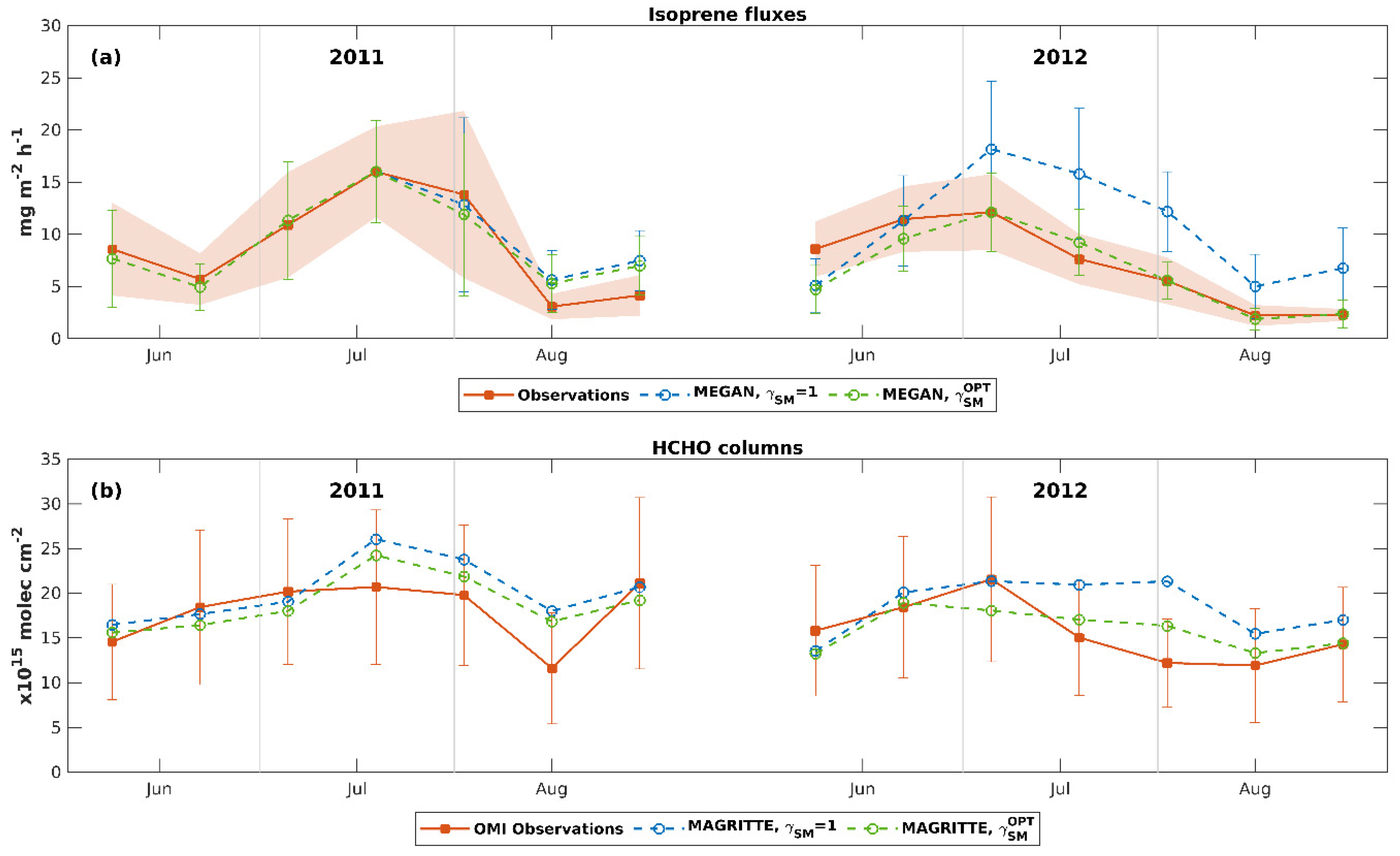
3.3. Local and Regional Simulations of Formaldehyde Columns

Here we examine the impact of drought stress on the temporal variability of isoprene fluxes and HCHO columns at the MOFLUX site. Both observed and calculated data are averaged biweekly (14 days) (Figure 5) and monthly (

Table 1. Monthly averages of (a–c) local isoprene fluxes (in mg m⁻² h⁻¹) from observations and MEGAN estimations (MEGAN, ${\gamma }_{SM}=1$ and MEGAN, ${\gamma }_{SM}^{OPT}$); (d–g) formaldehyde columns (in 10¹⁵ molecules cm⁻²) observed by OMI sensor around the MOFLUX site and calculated by MAGRITTE with biogenic emissions in no-stress conditions (MAGRITTE, ${\gamma }_{SM}=1$) and applying the drought stress factor (MAGRITTE, ${\gamma }_{SM}^{0.04}$ and MAGRITTE, ${\gamma }_{SM}^{OPT}$). Relative changes (RC) are provided between monthly averages in years 2011 and 2012 as percentages. The relative changes in OMI columns are provided along with their uncertainty estimates at 1σ-level calculated based on random uncertainties of columns retrievals.

	June			July			August
	2011	2012	RC (%)	2011	2012	RC (%)	2011	2012	RC (%)
(a) Observed isoprene flux	7.3	10.7	+47	14.4	9.0	−38	7.2	3.4	−53
(b) MEGAN, ${\gamma }_{SM}=1$	6.3	9.9	+60	14.2	16.6	+16	9.2	7.9	−14
(c) MEGAN, ${\gamma }_{SM}^{OPT}$	6.3	8.4	+34	14.2	10.1	−29	8.4	3.1	−63
(d) OMI HCHO column	16.2	17.5	+8 (±22)	21.9	17.7	−19 (±13)	16.2	12.5	−23 (±20)
(e) MAGRITTE HCHO column with ${\gamma }_{SM}=1$	16.9	17.6	+4	24.5	22.2	−10	20.6	16.3	−21
(f) MAGRITTE HCHO column with ${\gamma }_{SM}^{0.04}$	16.5	17.5	+6	24.1	22.1	−8	20.1	16.0	−20
(g) MAGRITTE HCHO column with ${\gamma }_{SM}^{OPT}$	15.9	16.9	+6	23.0	18.4	−20	19.3	13.9	−28

). As seen in Figure 3, isoprene fluxes exhibit great temporal variability at short timescales, but its evaluation using OMI HCHO observations cannot be performed due to the high noise and limited set of valid data (Section S2 of the Supplementary Materials).

Observed biweekly OMI HCHO columns averaged over a 20-km radius around the site (Figure 5b) follow essentially the same pattern as in situ measured isoprene fluxes (Figure 5a), although with a dampened amplitude. This dampening is expected due to the presence of other HCHO precursors less affected by drought (e.g., methane, methanol and anthropogenic VOCs) and due to complex transport and chemical effects, as discussed for instance by [41]. MAGRITTE simulations show the same biweekly variability during summer 2011, with HCHO columns reduced when using the drought factor ${\gamma }_{SM}^{OPT}$. Whereas the observed columns are relatively constant in July and early August, MAGRITTE simulations exhibit a greater biweekly variability with a mid-July peak, reflecting the temporal variability of isoprene fluxes. In 2012, OMI observations display a strong decline of HCHO column following the peak in early July, which is not reproduced by MAGRITTE simulations. Overall, application of the drought factor ${\gamma }_{SM}^{OPT}$ reduces the positive biases in biweekly averages of HCHO columns estimated in the no-stress simulation as shown in Figure 5b. Note however that the OMI systematic errors are important, of the order of 50%, and encompass both MAGRITTE simulations, except in early August 2012.

Monthly isoprene fluxes were enhanced in June 2012 compared to the previous year (Figure 5a and Table 1). More favourable (i.e., warm and sunny) environmental conditions at the onset of the severe drought explain this increase, as shown by the model ability to match the large emission enhancement in June (+47% in the observations and 34–60% in the model). In subsequent months, observed isoprene fluxes were about 40% and 50% lower than in the previous year, representing drastic decreases relative to the model expectation ignoring drought stress effects (+16% and −14% in July and August, respectively). The updated MEGAN model based on ${\gamma }_{SM}^{OPT}$ reproduces fairly well the seasonal variation (Figure 5a) as well as the inter-annual variability of summer monthly averages (Table 1).

A peak was observed in OMI HCHO in July 2011 at about 22 × 10¹⁵ molecules cm⁻² mainly due to high temperatures entailing fast VOC oxidation and strong biogenic emissions. About half this column was observed in August 2012 (12.5 × 10¹⁵ molecules cm⁻²) when severe drought took its toll on biogenic emissions. While the small increase observed in June 2012 with respect to the previous year (+7%) is well simulated in all runs, the substantial drop in July (−19%) is very well represented in MAGRITTE,${\gamma }_{SM}^{OPT}$ (−20%), whereas MAGRITTE,${\gamma }_{SM}=1$ and MAGRITTE, ${\gamma }_{SM}^{0.04}$ barely account for half of that reduction (Table 1). Yet in August, the relative impact of drought in MAGRITTE,${\gamma }_{SM}^{OPT}$ is slightly overestimated (−28% vs. −23% in OMI). While those comparisons point to a better performance of MAGRITTE, ${\gamma }_{SM}^{OPT}$ at reproducing the interannual variability of monthly averaged HCHO columns, uncertainties in OMI relative changes (given between brackets in Table 1) do not allow for a robust conclusion to be drawn. In particular, in June, the uncertainty (±22%) exceeds the relative change (+8%).

Further, we assess the absolute difference in HCHO columns of 2012 and 2011 observed by OMI and modelled by MAGRITTE with ${\gamma }_{SM}=1$ and ${\gamma }_{SM}^{OPT}$ (Figure 6). Two regions depicted in Figure 6, where MAGRITTE predicts significant impacts of the drought stress effect, namely Texas (hereafter TX) and southeast U.S. (hereafter SEUS), are examined. Grid cells that are marked by a stippling are those for which the 2011 and 2012 columns are not statistically different (at the 68% confidence level), based on the random error estimates provided with the HCHO product.

A strong enhancement in 2012 columns over TX is observed by OMI, particularly in June but also in August. Since the area is primarily covered by prairie grasslands, HCHO columns are lower over central and west TX compared to the SEUS. The severe drought that hit Texas during the summer of 2011 (https://www.drought.gov/states/texas, accessed on 1 September 2021) led to enhanced temperatures and PAR (Figure S3) and to lower humidity levels in comparison with 2012. The strong regional enhancement over TX observed in OMI, +21% of relative change (RC) on average (

Table 2. Monthly HCHO columns (10¹⁵ molecules cm⁻²) in JJA 2011 and 2012 averaged over the Texas (TX) and southeast U.S. (SEUS) regions, and relative change (RC) between monthly averages in years 2012 relative to 2011 expressed in percentage. Values are given for OMI observations and for MAGRITTE, ${\gamma }_{SM}=1$ and MAGRITTE, ${\gamma }_{SM}^{OPT}$. The RC in OMI HCHO averaged columns is provided with the uncertainty based on the propagation of random errors of OMI columns.

		OMI			$\mathbf{MAGRITTE}, {\mathit{\gamma }}_{\mathit{S}\mathit{M}}=1$			$\mathbf{MAGRITTE}, {\mathit{\gamma }}_{\mathit{S}\mathit{M}}^{\mathit{O}\mathit{P}\mathit{T}}$
		June	July	August	June	July	August	June	July	August
TX	2011	11.2	12.8	14.0	13.4	14.5	17.4	10.8	11.2	12.1
	2012	13.5	12.6	13.7	13.8	13.0	15.6	12.3	11.4	12.7
	RC (%)	+21 (±23)	−1 (±18)	−2 (±17)	+3	−10	−10	+14	+2	+5
SEUS	2011	16.6	17.3	16.4	18.7	20.0	21.2	17.1	18.4	18.8
	2012	16.2	17.0	14.0	17.2	20.1	16.3	16.7	18.5	15.0
	RC (%)	−3 (±17)	−2 (±17)	−14 (±18)	−8	0	−23	−3	+1	−20

), is largely underestimated by the run ignoring drought stress (MAGRITTE, ${\gamma }_{SM}=1$) (+3%) because the faster VOC oxidation rate in 2012 (due to higher OH concentrations) and higher HCHO photolysis rate in 2011 (due to high radiation levels) were compensated by lower isoprene emissions in 2012 (due to lower temperatures and PAR). The model agreement with OMI greatly improves MAGRITTE, ${\gamma }_{SM}^{OPT}$ run 3, when accounting for ${\gamma }_{SM}^{OPT}$. The activity factor decreased biogenic emissions over east Texas in June 2012, leading to enhanced differences (14%) in HCHO columns over the TX region. In subsequent months, the activity factor also improves the prediction of the column differences between 2011 and 2012, from −10% in MAGRITTE, ${\gamma }_{SM}=1$ to small positive changes. While the average change has been improved due to the inclusion of stress, its spatial distribution has not. For instance, MAGRITTE, ${\gamma }_{SM}=1$ run 1 is in better agreement with OMI observations than MAGRITTE, ${\gamma }_{SM}^{OPT}$ in East Texas (Piney Woods), pointing to an overestimated drought stress effect in this region. This region exhibits relatively high HCHO columns due to the important source of isoprene oxidation stemming from the presence of a mixed evergreen-deciduous forestland and the 2012–2011 absolute difference in temperatures (Figure S3) plays a dominant role in this interannual variation of isoprene emissions.

The southeastern forests, a dense temperate trees coverage, extend from east Texas (Piney Woods) to North Carolina. HCHO columns in SEUS are primarily attributed to the oxidation of non-methane VOC due to the high biogenic isoprene and monoterpene emissions [41,42,62]. The region experienced lower temperatures and PAR in June and August 2012 (Figure S3) which explains to a great extent the negative 2012-to-2011 HCHO differences observed by OMI and captured by the model, whereas opposite patterns are found in July. OMI observations in the SEUS show slight decreases in 2012 averaged columns in June (−3%) and July (−2%) followed by a larger drop of −14% in August (Table 2). In June and August, the relative changes simulated by MAGRITTE, ${\gamma }_{SM}^{OPT}$ in SEUS amount to −3% and −20%, respectively, i.e., in overall better agreement than MAGRITTE, ${\gamma }_{SM}^{0.04}$ using the default parameter. The impact of the drought stress factor (Figure S4) is mainly localized in Louisiana–Arkansas–Missouri and Georgia. This corresponds well with the 2012 patterns reported by the U.S. Drought Monitor (https://www.ncdc.noaa.gov/sotc/drought/201208, accessed on 1 September 2021).

While average columns and relative changes point to an overall better agreement when using the optimized drought factor (with MAGRITTE, ${\gamma }_{SM}^{OPT}$, the uncertainties in OMI HCHO retrievals undermine the confidence in this result. Based on the random error estimates provided with the QA4ECV HCHO product, only about 50% of the differences shown on Figure 6 are statistically different from zero at 1σ (20% at 2σ i.e., 95% confidence level). Moreover, Table 2 shows that the uncertainty in the OMI relative changes based on the estimated random uncertainties of the OMI retrieval, is of the order of 20%, which is higher than (or of the same order as) the relative changes in OMI HCHO averaged columns. Both MAGRITTE-calculated column differences lie within the error bar of the observations. Note that the filtering of OMI data based on AOD and GFED emissions (aimed to minimize the potential impact of biomass burning and aerosols) does not change the conclusions (Section S6 of the Supplement). The filtering leads to a decrease in the number of observations, most pronounced in the SEUS (Figure S5), which increases the noise level and leads to enhanced column differences (Figure S6). On average over the TX and SEUS regions, however, the relative differences (Table S2) are very similar to those of Table 2.

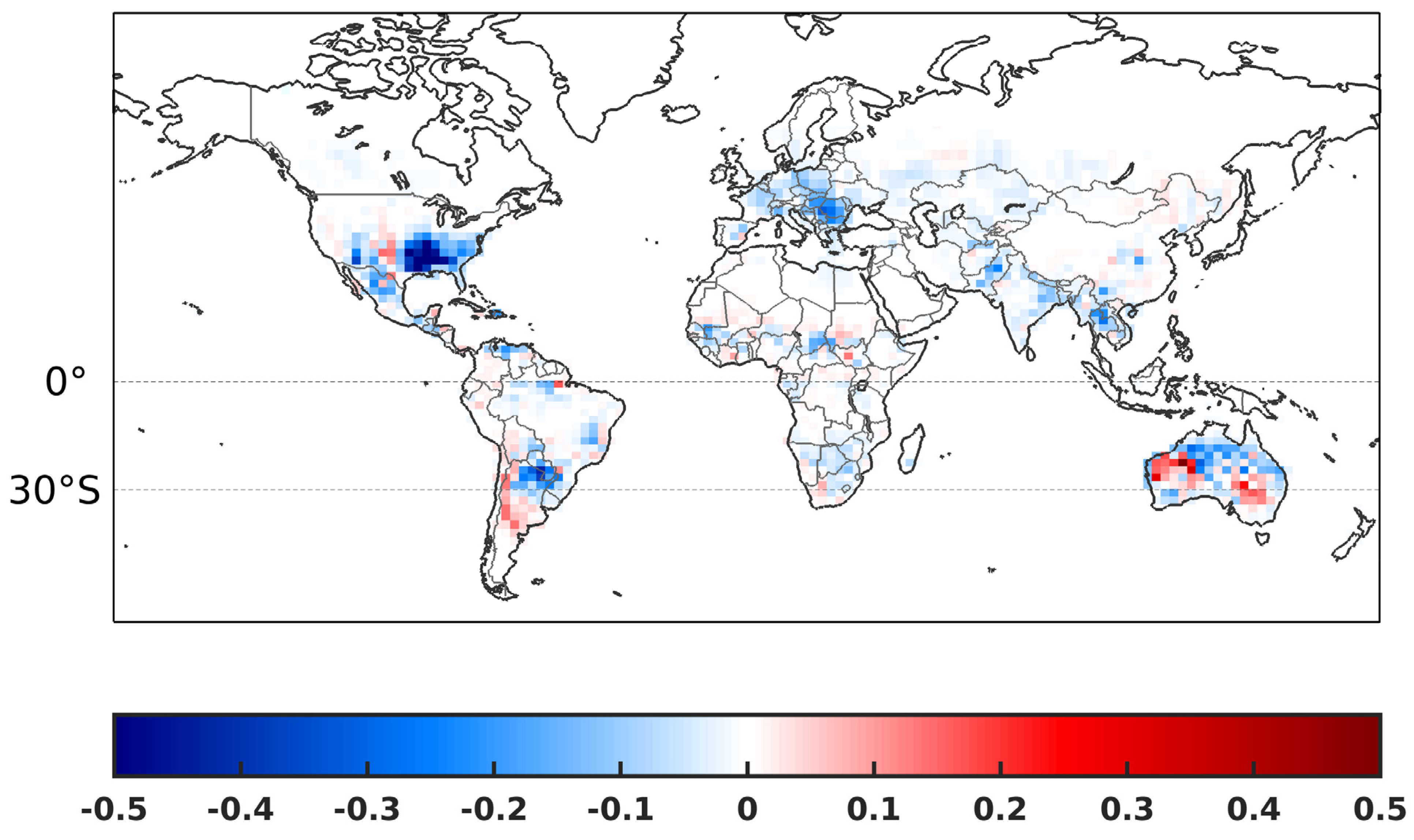
3.4. Global Simulations of HCHO Columns

The interannual variability in seasonal averages from global simulations modelled by IMAGES over the course of 2005–2016 is assessed against OMI HCHO columns (Figure S7). Figure 7 displays the difference in correlation coefficients between two runs, IMAGES, ${\gamma }_{SM}^{0.04}$ and IMAGES, ${\gamma }_{SM}^{OPT}$. The seasonal averages are calculated over the months of June–August in the Northern Hemisphere (>0°N), February–April in the 0°–30°S latitudinal band, and December–February below the 30th parallel, corresponding to months with low biomass burning activity.

Overall, the correlation coefficient in the interannual variability in HCHO columns is deteriorated in IMAGES, ${\gamma }_{SM}^{OPT}$ compared to IMAGES, ${\gamma }_{SM}^{0.04}$, particularly, in southeastern U.S., the Gran Chaco (vicinity of Paraguay), eastern and southeastern Europe, and northern Australia. Those regions exhibit relatively high isoprene emissions (e.g., [6]) that lead to high, statistically significant correlations in HCHO in IMAGES, ${\gamma }_{SM}^{0.04}$ (Figure S7a). But stronger reductions in isoprene emissions in these areas due to the adjusted parameterization are not supported by OMI observations. Correlations are slightly improved in arid or semi-arid regions such as the Great Plains (central U.S.), shrubland of Western Australia, and the Argentinian Monte desert. Due to the sparse vegetation found in these regions, emissions of isoprene are of a lesser magnitude and the poor agreement between IMAGES, ${\gamma }_{SM}^{0.04}$ and OMI observations is found in these vicinities (Figure S7a) is likely due to the relatively low HCHO signal. As a result, improved correlations shown in Figure 7 remain statistically insignificant (Figure S7b). The filtering of OMI data for high AOD and pyrogenic emissions have only a minimal impact on the conclusions of the global model analysis (Figure S8). The filtering slightly decreases, as expected, the temporal correlation between the monthly HCHO columns from the model and the observation, due to degraded statistics, but the filtered dataset leads to the same patterns as seen in Figure 7.

4. Discussion and Conclusions

Previous studies conducted on the MOFLUX site noted that the low value of wilting point used in the default parameterization of MEGANv2.1 at this site (0.084 m³ m⁻³, [103]) prevent the stress factor from capturing the effect of drought on isoprene emissions [30,32,52,68]. In this study, we focused on optimizing the empirical parameter $\Delta \theta$ of the MEGANv2.1 soil moisture stress algorithm. The parameter $\Delta \theta$ was originally set to 0.06 [48] and was later re-evaluated to a lower, more conservative, value of 0.04 m³ m⁻³ [5] so that the emissions are shut off only in extreme drought conditions. Here we re-evaluated it ($\Delta \theta =0.12$) based on isoprene flux measurements at the MOFLUX site conducted in mild and severe drought conditions, and GLEAM soil moisture. The adjusted parameterization leads to an improved prediction of daily isoprene emissions rates during the severe drought at the MOFLUX site (r = 0.90, RMSE = 2.02 mg m⁻² h⁻¹) compared to the no-stress simulation (r = 0.76, RMSE = 4.98 mg m⁻² h⁻¹) and to the simulation adopting the MEGANv3 parameterization (r = 0.79, RMSE = 3.13 mg m⁻² h⁻¹). Analysis of OMI and modelled tropospheric HCHO column over the MOFLUX site supports this conclusion. At a regional scale, the relative changes in simulated formaldehyde between the two years show some improvement when including the adapted parameterization over certain regions in the U.S., but clearly not over all areas. Nonetheless, global long-term HCHO simulations using ${\gamma }_{SM}^{OPT}$ lead to heterogeneous results, with extended areas where the correlation with OMI observations worsens compared to the use of the default parameterization.

The study is subject to limitations and uncertainties. Foremost, the adjustment of the parameter $\Delta \theta$ is influenced by many factors including the $\theta$ dataset, the soil depth of reference, and the MEGAN parametrized response functions to environmental conditions other than soil moisture. For instance, using in situ measurements of the $\theta$ at 100 cm and the local wilting point (0.23 m³ m⁻³), the optimized $\Delta \theta$ would be about twice higher (0.25 m³ m⁻³) than the value derived using GLEAM $\theta$ (0.12 m³ m⁻³). In addition, the high sensitivity of isoprene emissions to soil properties using the MEGANv2.1 parameterization has been demonstrated in numerous studies and motivated the adoption of higher values of $\Delta \theta$ despite the earlier rationale to only apply the isoprene reduction for extreme droughts, that led to its downward revision. Also, soil moisture should be seen as relative, i.e., framed by the soil properties the model uses. In particular, the high heterogeneity of porosity renders soil properties inaccurate since they are a function of porosity, such that the comparison of soil moisture in absolute terms is of limited relevance. Consistency in the use of soil characteristics dataset is also crucial as already pointed out in [49]. For year 2012, Seco et al. (2015) [32] used the MEGANv2.1 drought activity factor algorithm with the measured $\theta$ data at 10 cm jointly with the local wilting point (0.23 m³ m⁻³) and found a substantial improvement in the overall model results against the MOFLUX isoprene flux measurements. However, the wilting point of 0.13 m³ m⁻³ for the top 30 cm (Section 2.1) would be more appropriate when using the 10 cm $\theta$ data. Therefore, since the $\theta$ measured at 10 cm always exceeds the threshold of 0.13 + 0.04 = 0.17 m³ m⁻³, no drought stress is predicted by MEGANv2.1 based on 10 cm $\theta$ data. The level at which the $\theta$ is defined is important due to the general increase of $\theta$ with depth and to changes in the temporal evolution due to water percolation.

Regarding the assessment of drought impacts using formaldehyde columns, the following shortcomings and limitations are raised. OMI HCHO observations lack the precision required to conduct an evaluation on isoprene emission estimates at short temporal scales (daily and weekly), which would be most relevant for drought impact studies. With its much higher resolution and increased sensitivity to day-to-day variability [102], the TROPOMI sensor on Sentinel-5p offers promising perspectives for future research. As we have seen, the exclusion of OMI data characterized by high AOD or high pyrogenic emissions degrades the statistics while not fundamentally affecting the conclusions of the study. Modelled tropospheric HCHO columns over the MOFLUX site pointed to an overall better agreement with the adjusted parameterization and the radius of 20 km was chosen as the best for representing the site given that satellite overpasses within a smaller radius were too infrequent (<17/month for 10 km). At greater coverage (30 km), however, the MAGRITTE runs with the least soil moisture stress (as in MAGRITTE, ${\gamma }_{SM}=1$ and MAGRITTE, ${\gamma }_{SM}^{0.04}$) are in best overall agreement with OMI observations (Table S1). At the global scale, high values of $\Delta \theta$ are not supported by observations. Indeed, multi-year global simulations (2005–2016) with the CTM IMAGES indicated that the use of $\Delta \theta$ = 0.12 m³ m⁻³ does not improve significantly the comparison with OMI HCHO over dry regions, and it worsens the comparison over most forested areas. The best agreement with OMI in terms of interannual variability is found when the drought activity factor is not accounted for (not shown here). The reason for such disparity between the MOFLUX study and the large-scale evaluation using HCHO could lie in the spatial resolution. Disparities in soil water content between local and grid cell scales can be huge given the great heterogeneity in soil properties like porosity and subsequently for the ‘absolute’ values of soil moisture and the empirical parameter. Another issue with the current parameterization is that it is independent of various environmental factors other than the soil moisture characteristics. Furthermore, the response of isoprene emissions depends on the drought characteristics and plant species. The parametrization of drought stress should account for different effects across biomes and species [104,105,106]. For instance, Genard-Zielinski et al. (2018) [39] suggested an exponential reduction function of the SWC for drought-adapted species. In addition, longer and recurrent drought (e.g., 10 years) could have progressive and cumulative effects over time in forested ecosystems dominated by long-lived species [18]. Besides the complexity of the drought response, the lack of ecosystem-scale, long-term monitoring of soil moisture and isoprene emissions is another important issue. Direct comparison between MEGAN and flux measurements in various drought conditions has been only possible for the MOFLUX site. Other campaigns including isoprene concentration measurements in drought-impacted ecosystems ([39,40]) provide qualitative insights but no direct constraint on the fluxes. A possible avenue for drought stress parameterizations could be the development of empirical relationships making use of remotely sensed photosynthetic parameters or vegetation indices such as SIF [47], Emissivity Difference Vegetation Index (EDVI; [107]) or Photochemical Reflectance Index (PRI; [108]). So far, however, progress has been limited in that direction.

References

1. Fehsenfeld, F.; Calvert, J.; Fall, R.; Goldan, P.; Guenther, A.B.; Hewitt, C.N.; Lamb, B.; Liu, S.; Trainer, M.; Westberg, H.; et al. Emissions of Volatile Organic Compounds from Vegetation and the Implications for Atmospheric Chemistry. Glob. Biogeochem. Cycles 1992, 6, 389–430. [Google Scholar] [CrossRef]
2. Atkinson, R. Atmospheric Chemistry of VOCs and NOx. Atmos. Environ. 2000, 34, 2063–2101. [Google Scholar] [CrossRef]
3. Pike, R.C.; Young, P.J. How Plants Can Influence Tropospheric Chemistry: The Role of Isoprene Emissions from the Biosphere. Weather 2009, 64, 332–336. [Google Scholar] [CrossRef] [Green Version]
4. Lathière, J.; Hauglustaine, D.A.; Friend, A.D.; De Noblet-Ducoudré, N.; Viovy, N.; Folberth, G.A. Impact of Climate Variability and Land Use Changes on Global Biogenic Volatile Organic Compound Emissions. Atmos. Chem. Phys. 2006, 6, 2129–2146. [Google Scholar] [CrossRef] [Green Version]
5. Guenther, A.B.; Jiang, X.; Heald, C.L.; Sakulyanontvittaya, T.; Duhl, T.; Emmons, L.K.; Wang, X. The Model of Emissions of Gases and Aerosols from Nature Version 2.1 (MEGAN2.1): An Extended and Updated Framework for Modeling Biogenic Emissions. Geosci. Model Dev. 2012, 5, 1471–1492. [Google Scholar] [CrossRef] [Green Version]
6. Sindelarova, K.; Granier, C.; Bouarar, I.; Guenther, A.; Tilmes, S.; Stavrakou, T.; Müller, J.-F.; Kuhn, U.; Stefani, P.; Knorr, W. Global Data Set of Biogenic VOC Emissions Calculated by the MEGAN Model over the Last 30 Years. Atmos. Chem. Phys. 2014, 14, 9317–9341. [Google Scholar] [CrossRef] [Green Version]
7. Messina, P.; Lathière, J.; Sindelarova, K.; Vuichard, N.; Granier, C.; Ghattas, J.; Cozic, A.; Hauglustaine, D.A. Global Biogenic Volatile Organic Compound Emissions in the ORCHIDEE and MEGAN Models and Sensitivity to Key Parameters. Atmos. Chem. Phys. 2016, 16, 14169–14202. [Google Scholar] [CrossRef] [Green Version]
8. Granier, C.; Darras, S.; Denier van der Gon, H.; Doubalova, J.; Elguindi, N.; Galle, B.; Gauss, M.; Guevara, M.; Jalkanen, J.-P.; Kuenen, J.; et al. The Copernicus Atmosphere Monitoring Service Global and Regional Emissions (April 2019 Version). Copernic. Atmos. Monit. Serv. 2019. [Google Scholar] [CrossRef]
9. Lelieveld, J.; Butler, T.; Crowley, J.; Dillon, T.; Fischer, H.; Ganzeveld, L.; Harder, H.; Lawrence, M.; Martinez, M.; Taraborrelli, D.; et al. Atmospheric Oxidation Capacity Sustained by a Tropical Forest. Nature 2008, 452, 737–740. [Google Scholar] [CrossRef]
10. Hofzumahaus, A.; Rohrer, F.; Lu, K.; Bohn, B.; Brauers, T.; Chang, C.-C.; Fuchs, H.; Holland, F.; Kita, K.; Kondo, Y.; et al. Amplified Trace Gas Removal in the Troposphere. Science 2009, 324, 1702–1704. [Google Scholar] [CrossRef] [Green Version]
11. Peeters, J.; Nguyen, T.L.; Vereecken, L. HOx Radical Regeneration in the Oxidation of Isoprene. Phys. Chem. Chem. Phys. 2009, 11, 5935–5939. [Google Scholar] [CrossRef]
12. Peeters, J.; Müller, J.-F. HOx Radical Regeneration in Isoprene Oxidation via Peroxy Radical Isomerisations. II: Experimental Evidence and Global Impact. Phys. Chem. Chem. Phys. 2010, 12, 14227–14235. [Google Scholar] [CrossRef] [PubMed]
13. Fuchs, H.; Hofzumahaus, A.; Rohrer, F.; Bohn, B.; Brauers, T.; Dorn, H.-P.; Häseler, R.; Holland, F.; Kaminski, M.; Li, X.; et al. Experimental Evidence for Efficient Hydroxyl Radical Regeneration in Isoprene Oxidation. Nat. Geosci. 2013, 6, 1023–1026. [Google Scholar] [CrossRef]
14. Hansen, R.F.; Lewis, T.R.; Graham, L.; Whalley, L.K.; Seakins, P.W.; Heard, D.E.; Blitz, M.A. OH Production from the Photolysis of Isoprene-Derived Peroxy Radicals: Cross-Sections, Quantum Yields and Atmospheric Implications. Phys. Chem. Chem. Phys. 2017, 19, 2332–2345. [Google Scholar] [CrossRef] [PubMed]
15. Ryerson, T.B.; Trainer, M.; Holloway, J.S.; Parrish, D.D.; Huey, L.G.; Sueper, D.T.; Frost, G.J.; Donnelly, S.G.; Schauffler, S.; Atlas, E.L.; et al. Observations of Ozone Formation in Power Plant Plumes and Implications for Ozone Control Strategies. Science 2001, 292, 719–723. [Google Scholar] [CrossRef] [Green Version]
16. Da Silva, C.M.; Corrêa, S.M.; Arbilla, G. Isoprene Emissions and Ozone Formation in Urban Conditions: A Case Study in the City of Rio de Janeiro. Bull. Environ. Contam. Toxicol. 2018, 100, 184–188. [Google Scholar] [CrossRef] [PubMed]
17. Mo, Z.; Shao, M.; Wang, W.; Liu, Y.; Wang, M.; Lu, S. Evaluation of Biogenic Isoprene Emissions and Their Contribution to Ozone Formation by Ground-Based Measurements in Beijing, China. Sci. Total Environ. 2018, 627, 1485–1494. [Google Scholar] [CrossRef] [PubMed]
18. Saunier, A.; Ormeño, E.; Piga, D.; Armengaud, A.; Boissard, C.; Lathière, J.; Szopa, S.; Genard-Zielinski, A.-C.; Fernandez, C. Isoprene Contribution to Ozone Production under Climate Change Conditions in the French Mediterranean Area. Reg. Environ. Chang. 2020, 20, 111. [Google Scholar] [CrossRef]
19. Claeys, M.; Graham, B.; Vas, G.; Wang, W.; Vermeylen, R.; Pashynska, V.; Cafmeyer, J.; Guyon, P.; Andreae, M.; Artaxo, P.; et al. Formation of Secondary Organic Aerosols through Photooxidation of Isoprene. Science 2004, 303, 1173–1176. [Google Scholar] [CrossRef] [PubMed] [Green Version]
20. Kroll, J.H.; Ng, N.L.; Murphy, S.M.; Flagan, R.C.; Seinfeld, J.H. Secondary Organic Aerosol Formation from Isoprene Photooxidation under High-NOx Conditions. Geophys. Res. Lett. 2005, 32. [Google Scholar] [CrossRef] [Green Version]
21. Kroll, J.H.; Ng, N.L.; Murphy, S.M.; Flagan, R.C.; Seinfeld, J.H. Secondary Organic Aerosol Formation from Isoprene Photooxidation. Environ. Sci. Technol. 2006, 40, 1869–1877. [Google Scholar] [CrossRef] [PubMed] [Green Version]
22. Carlton, A.G.; Wiedinmyer, C.; Kroll, J.H. A Review of Secondary Organic Aerosol (SOA) Formation from Isoprene. Atmos. Chem. Phys. 2009, 9, 4987–5005. [Google Scholar] [CrossRef] [Green Version]
23. Tingey, D.T.; Evans, R.; Gumpertz, M. Effects of Environmental Conditions on Isoprene Emission from Live Oak. Planta 1981, 152, 565–570. [Google Scholar] [CrossRef] [PubMed]
24. Sharkey, T.D.; Loreto, F. Water Stress, Temperature, and Light Effects on the Capacity for Isoprene Emission and Photosynthesis of Kudzu Leaves. Oecologia 1993, 95, 328–333. [Google Scholar] [CrossRef]
25. Funk, J.L.; Jones, C.G.; Gray, D.W.; Throop, H.L.; Hyatt, L.A.; Lerdau, M.T. Variation in Isoprene Emission from Quercus Rubra: Sources, Causes, and Consequences for Estimating Fluxes. J. Geophys. Res. Atmos. 2005, 110. [Google Scholar] [CrossRef] [Green Version]
26. Singsaas, E.L.; Lerdau, M.; Winter, K.; Sharkey, T.D. Isoprene Increases Thermotolerance of Isoprene-Emitting Species. Plant Physiol. 1997, 115, 1413–1420. [Google Scholar] [CrossRef] [PubMed] [Green Version]
27. Sharkey, T.D.; Chen, X.; Yeh, S. Isoprene Increases Thermotolerance of Fosmidomycin-Fed Leaves. Plant Physiol. 2001, 125, 2001–2006. [Google Scholar] [CrossRef] [PubMed] [Green Version]
28. Sasaki, K.; Saito, T.; Lämsä, M.; Oksman-Caldentey, K.-M.; Suzuki, M.; Ohyama, K.; Muranaka, T.; Ohara, K.; Yazaki, K. Plants Utilize Isoprene Emission as a Thermotolerance Mechanism. Plant Cell Physiol. 2007, 48, 1254–1262. [Google Scholar] [CrossRef] [PubMed] [Green Version]
29. Niinemets, Ü.; Copolovici, L.; Hüve, K. High Within-Canopy Variation in Isoprene Emission Potentials in Temperate Trees: Implications for Predicting Canopy-Scale Isoprene Fluxes. J. Geophys. Res. Biogeosci. 2010, 115. [Google Scholar] [CrossRef] [Green Version]
30. Potosnak, M.J.; LeStourgeon, L.; Pallardy, S.G.; Hosman, K.P.; Gu, L.; Karl, T.; Geron, C.; Guenther, A.B. Observed and Modeled Ecosystem Isoprene Fluxes from an Oak-Dominated Temperate Forest and the Influence of Drought Stress. Atmos. Environ. 2014, 84, 314–322. [Google Scholar] [CrossRef] [Green Version]
31. Brüggemann, N.; Schnitzler, J.-P. Comparison of Isoprene Emission, Intercellular Isoprene Concentration and Photosynthetic Performance in Water-Limited Oak (Quercus pubescens Willd. and Quercus robur L.) Saplings. Plant Biol. 2002, 4, 456–463. [Google Scholar] [CrossRef]
32. Seco, R.; Karl, T.; Guenther, A.; Hosman, K.P.; Pallardy, S.G.; Gu, L.; Geron, C.; Harley, P.; Kim, S. Ecosystem-Scale Volatile Organic Compound Fluxes during an Extreme Drought in a Broadleaf Temperate Forest of the Missouri Ozarks (Central USA). Glob. Chang. Biol. 2015, 21, 3657–3674. [Google Scholar] [CrossRef] [Green Version]
33. Pegoraro, E.; Rey, A.; Greenberg, J.; Harley, P.; Grace, J.; Malhi, Y.; Guenther, A. Effect of Drought on Isoprene Emission Rates from Leaves of Quercus Virginiana Mill. Atmos. Environ. 2004, 38, 6149–6156. [Google Scholar] [CrossRef] [Green Version]
34. Funk, J.L.; Mak, J.E.; Lerdau, M.T. Stress-Induced Changes in Carbon Sources for Isoprene Production in Populus Deltoides. Plant Cell Environ. 2004, 27, 747–755. [Google Scholar] [CrossRef]
35. Brilli, F.; Barta, C.; Fortunati, A.; Lerdau, M.; Loreto, F.; Centritto, M. Response of Isoprene Emission and Carbon Metabolism to Drought in White Poplar (Populus Alba) Saplings. New Phytol. 2007, 175, 244–254. [Google Scholar] [CrossRef]
36. Centritto, M.; Brilli, F.; Fodale, R.; Loreto, F. Different Sensitivity of Isoprene Emission, Respiration and Photosynthesis to High Growth Temperature Coupled with Drought Stress in Black Poplar (Populus Nigra) Saplings. Tree Physiol. 2011, 31, 275–286. [Google Scholar] [CrossRef] [Green Version]
37. Tattini, M.; Loreto, F.; Fini, A.; Guidi, L.; Brunetti, C.; Velikova, V.; Gori, A.; Ferrini, F. Isoprenoids and Phenylpropanoids Are Part of the Antioxidant Defense Orchestrated Daily by Drought-Stressed Platanus × Acerifolia Plants during Mediterranean Summers. New Phytol. 2015, 207, 613–626. [Google Scholar] [CrossRef]
38. Bamberger, I.; Ruehr, N.K.; Schmitt, M.; Gast, A.; Wohlfahrt, G.; Arneth, A. Isoprene Emission and Photosynthesis during Heatwaves and Drought in Black Locust. Biogeosciences 2017, 14, 3649–3667. [Google Scholar] [CrossRef] [Green Version]
39. Genard-Zielinski, A.-C.; Boissard, C.; Ormeño, E.; Lathière, J.; Reiter, I.M.; Wortham, H.; Orts, J.-P.; Temime-Roussel, B.; Guenet, B.; Bartsch, S.; et al. Seasonal Variations of Quercus Pubescens Isoprene Emissions from an in Natura Forest under Drought Stress and Sensitivity to Future Climate Change in the Mediterranean Area. Biogeosciences 2018, 15, 4711–4730. [Google Scholar] [CrossRef]
40. Ferracci, V.; Bolas, C.G.; Freshwater, R.A.; Staniaszek, Z.; King, T.; Jaars, K.; Otu-Larbi, F.; Beale, J.; Malhi, Y.; Waine, T.W.; et al. Continuous Isoprene Measurements in a UK Temperate Forest for a Whole Growing Season: Effects of Drought Stress During the 2018 Heatwave. Geophys. Res. Lett. 2020, 47, e2020GL088885. [Google Scholar] [CrossRef]
41. Palmer, P.I.; Jacob, D.J.; Fiore, A.M.; Martin, R.V.; Chance, K.; Kurosu, T.P. Mapping Isoprene Emissions over North America Using Formaldehyde Column Observations from Space. J. Geophys. Res. Atmos. 2003, 108. [Google Scholar] [CrossRef] [Green Version]
42. Millet, D.B.; Jacob, D.J.; Boersma, K.F.; Fu, T.-M.; Kurosu, T.P.; Chance, K.; Heald, C.L.; Guenther, A. Spatial Distribution of Isoprene Emissions from North America Derived from Formaldehyde Column Measurements by the OMI Satellite Sensor. J. Geophys. Res. Atmos. 2008, 113. [Google Scholar] [CrossRef]
43. Stavrakou, T.; Müller, J.-F.; De Smedt, I.; Van Roozendael, M.; van der Werf, G.R.; Giglio, L.; Guenther, A. Global Emissions of Non-Methane Hydrocarbons Deduced from SCIAMACHY Formaldehyde Columns through 2003–2006. Atmos. Chem. Phys. 2009, 9, 3663–3679. [Google Scholar] [CrossRef] [Green Version]
44. Cao, H.; Fu, T.-M.; Zhang, L.; Henze, D.K.; Miller, C.C.; Lerot, C.; Abad, G.G.; De Smedt, I.; Zhang, Q.; van Roozendael, M.; et al. Adjoint Inversion of Chinese Non-Methane Volatile Organic Compound Emissions Using Space-Based Observations of Formaldehyde and Glyoxal. Atmos. Chem. Phys. 2018, 18, 15017–15046. [Google Scholar] [CrossRef] [Green Version]
45. Bauwens, M.; Verreyken, B.; Stavrakou, T.; Müller, J.-F.; Smedt, I.D. Spaceborne Evidence for Significant Anthropogenic VOC Trends in Asian Cities over 2005–2019. Environ. Res. Lett. 2022, 17, 015008. [Google Scholar] [CrossRef]
46. Stavrakou, T.; Müller, J.-F.; Bauwens, M.; De Smedt, I.; Van Roozendael, M.; Guenther, A. Impact of Short-Term Climate Variability on Volatile Organic Compounds Emissions Assessed Using OMI Satellite Formaldehyde Observations. Geophys. Res. Lett. 2018, 45, 8681–8689. [Google Scholar] [CrossRef]
47. Zheng, Y.; Unger, N.; Tadić, J.M.; Seco, R.; Guenther, A.B.; Barkley, M.P.; Potosnak, M.J.; Murray, L.T.; Michalak, A.M.; Qiu, X.; et al. Drought Impacts on Photosynthesis, Isoprene Emission and Atmospheric Formaldehyde in a Mid-Latitude Forest. Atmos. Environ. 2017, 167, 190–201. [Google Scholar] [CrossRef] [Green Version]
48. Guenther, A.; Karl, T.; Harley, P.; Wiedinmyer, C.; Palmer, P.I.; Geron, C. Estimates of Global Terrestrial Isoprene Emissions Using MEGAN (Model of Emissions of Gases and Aerosols from Nature). Atmos. Chem. Phys. 2006, 6, 3181–3210. [Google Scholar] [CrossRef] [Green Version]
49. Müller, J.-F.; Stavrakou, T.; Wallens, S.; De Smedt, I.; Van Roozendael, M.; Potosnak, M.J.; Rinne, J.; Munger, B.; Goldstein, A.; Guenther, A.B. Global Isoprene Emissions Estimated Using MEGAN, ECMWF Analyses and a Detailed Canopy Environment Model. Atmos. Chem. Phys. 2008, 8, 1329–1341. [Google Scholar] [CrossRef] [Green Version]
50. Tawfik, A.B.; Stöckli, R.; Goldstein, A.; Pressley, S.; Steiner, A.L. Quantifying the Contribution of Environmental Factors to Isoprene Flux Interannual Variability. Atmos. Environ. 2012, 54, 216–224. [Google Scholar] [CrossRef]
51. Opacka, B.; Müller, J.-F.; Stavrakou, T.; Bauwens, M.; Sindelarova, K.; Markova, J.; Guenther, A.B. Global and Regional Impacts of Land Cover Changes on Isoprene Emissions Derived from Spaceborne Data and the MEGAN Model. Atmos. Chem. Phys. 2021, 21, 8413–8436. [Google Scholar] [CrossRef]
52. Huang, L.; McGaughey, G.; McDonald-Buller, E.; Kimura, Y.; Allen, D.T. Quantifying Regional, Seasonal and Interannual Contributions of Environmental Factors on Isoprene and Monoterpene Emissions Estimates over Eastern Texas. Atmos. Environ. 2015, 106, 120–128. [Google Scholar] [CrossRef]
53. Emmerson, K.M.; Palmer, P.I.; Thatcher, M.; Haverd, V.; Guenther, A.B. Sensitivity of Isoprene Emissions to Drought over South-Eastern Australia: Integrating Models and Satellite Observations of Soil Moisture. Atmos. Environ. 2019, 209, 112–124. [Google Scholar] [CrossRef]
54. Karthikeyan, L.; Pan, M.; Wanders, N.; Kumar, D.N.; Wood, E.F. Four Decades of Microwave Satellite Soil Moisture Observations: Part 1. A Review of Retrieval Algorithms. Adv. Water Resour. 2017, 109, 106–120. [Google Scholar] [CrossRef]
55. Miralles, D.G.; De Jeu, R.A.M.; Gash, J.H.; Holmes, T.R.H.; Dolman, A.J. An Application of GLEAM to Estimating Global Evaporation. Hydrol. Earth Syst. Sci. Discuss. 2011, 8, 1–27. [Google Scholar] [CrossRef] [Green Version]
56. Martens, B.; Miralles, D.G.; Lievens, H.; van der Schalie, R.; de Jeu, R.A.M.; Fernández-Prieto, D.; Beck, H.E.; Dorigo, W.A.; Verhoest, N.E.C. GLEAM v3: Satellite-Based Land Evaporation and Root-Zone Soil Moisture. Geosci. Model Dev. 2017, 10, 1903–1925. [Google Scholar] [CrossRef] [Green Version]
57. Gruber, A.; Scanlon, T.; van der Schalie, R.; Wagner, W.; Dorigo, W. Evolution of the ESA CCI Soil Moisture Climate Data Records and Their Underlying Merging Methodology. Earth Syst. Sci. Data 2019, 11, 717–739. [Google Scholar] [CrossRef] [Green Version]
58. Beck, H.E.; Pan, M.; Miralles, D.G.; Reichle, R.H.; Dorigo, W.A.; Hahn, S.; Sheffield, J.; Karthikeyan, L.; Balsamo, G.; Parinussa, R.M.; et al. Evaluation of 18 Satellite- and Model-Based Soil Moisture Products Using in Situ Measurements from 826 Sensors. Hydrol. Earth Syst. Sci. 2021, 25, 17–40. [Google Scholar] [CrossRef]
59. Palmer, P.I.; Abbot, D.S.; Fu, T.-M.; Jacob, D.J.; Chance, K.; Kurosu, T.P.; Guenther, A.; Wiedinmyer, C.; Stanton, J.C.; Pilling, M.J.; et al. Quantifying the Seasonal and Interannual Variability of North American Isoprene Emissions Using Satellite Observations of the Formaldehyde Column. J. Geophys. Res. Atmos. 2006, 111. [Google Scholar] [CrossRef] [Green Version]
60. Marais, E.A.; Jacob, D.J.; Kurosu, T.P.; Chance, K.; Murphy, J.G.; Reeves, C.; Mills, G.; Casadio, S.; Millet, D.B.; Barkley, M.P.; et al. Isoprene Emissions in Africa Inferred from OMI Observations of Formaldehyde Columns. Atmos. Chem. Phys. 2012, 12, 6219–6235. [Google Scholar] [CrossRef] [Green Version]
61. Bauwens, M.; Stavrakou, T.; Müller, J.-F.; De Smedt, I.; Van Roozendael, M.; van der Werf, G.R.; Wiedinmyer, C.; Kaiser, J.W.; Sindelarova, K.; Guenther, A. Nine Years of Global Hydrocarbon Emissions Based on Source Inversion of OMI Formaldehyde Observations. Atmos. Chem. Phys. 2016, 16, 10133–10158. [Google Scholar] [CrossRef] [Green Version]
62. Kaiser, J.; Jacob, D.J.; Zhu, L.; Travis, K.R.; Fisher, J.A.; González Abad, G.; Zhang, L.; Zhang, X.; Fried, A.; Crounse, J.D.; et al. High-Resolution Inversion of OMI Formaldehyde Columns to Quantify Isoprene Emission on Ecosystem-Relevant Scales: Application to the Southeast US. Atmos. Chem. Phys. 2018, 18, 5483–5497. [Google Scholar] [CrossRef] [Green Version]
63. Gu, L.; Meyers, T.; Pallardy, S.G.; Hanson, P.J.; Yang, B.; Heuer, M.; Hosman, K.P.; Riggs, J.S.; Sluss, D.; Wullschleger, S.D. Direct and Indirect Effects of Atmospheric Conditions and Soil Moisture on Surface Energy Partitioning Revealed by a Prolonged Drought at a Temperate Forest Site. J. Geophys. Res. Atmos. 2006, 111. [Google Scholar] [CrossRef]
64. Wood, J.D.; University of Missouri, Columbia, MO, USA. Personal Communication, 2021.
65. Tolk, J. Soils, Permanent Wilting Points; Howell, T.A., Stewart, B.A., Eds.; Marcel-Dekker, Inc.: New York, NY, USA, 2003; ISBN 0-8247-4241-9. [Google Scholar]
66. Hinckley, T.M.; Dougherty, P.M.; Lassoie, J.P.; Roberts, J.E.; Teskey, R.O. A Severe Drought: Impact on Tree Growth, Phenology, Net Photosynthetic Rate and Water Relations. Am. Midl. Nat. 1979, 102, 307–316. [Google Scholar] [CrossRef]
67. Bahari, Z.A.; Pallardy, S.G.; Parker, W.C. Photosynthesis, Water Relations, and Drought Adaptation in Six Woody Species of Oak-Hickory Forests in Central Missouri. For. Sci. 1985, 31, 557–569. [Google Scholar] [CrossRef]
68. Wallens, S. Modélisation Des Émissions de Composés Organiques Volatils Par La Végétation. Ph.D. Thesis, Universite Libre de Bruxelles, Brussels, Belgium, 2004. [Google Scholar]
69. Jiang, X.; Guenther, A.; Potosnak, M.; Geron, C.; Seco, R.; Karl, T.; Kim, S.; Gu, L.; Pallardy, S. Isoprene Emission Response to Drought and the Impact on Global Atmospheric Chemistry. Atmos. Environ. 2018, 183, 69–83. [Google Scholar] [CrossRef]
70. Oleson, K.; Lawrence, M.; Bonan, B.; Drewniak, B.; Huang, M.; Koven, D.; Levis, S.; Li, F.; Riley, J.; Subin, M.; et al. Technical Description of Version 4.5 of the Community Land Model (CLM); UCAR: Boulder, CO, USA, 2013. [Google Scholar]
71. Gent, P.R.; Danabasoglu, G.; Donner, L.J.; Holland, M.M.; Hunke, E.C.; Jayne, S.R.; Lawrence, D.M.; Neale, R.B.; Rasch, P.J.; Vertenstein, M.; et al. The Community Climate System Model Version 4. J. Clim. 2011, 24, 4973–4991. [Google Scholar] [CrossRef]
72. Priestley, C.H.B.; Taylor, R.J. On the Assessment of Surface Heat Flux and Evaporation Using Large-Scale Parameters. Mon. Weather Rev. 1972, 100, 81–92. [Google Scholar] [CrossRef]
73. Moesinger, L.; Dorigo, W.; de Jeu, R.; van der Schalie, R.; Scanlon, T.; Teubner, I.; Forkel, M. The Global Long-Term Microwave Vegetation Optical Depth Climate Archive (VODCA). Earth Syst. Sci. Data 2020, 12, 177–196. [Google Scholar] [CrossRef] [Green Version]
74. Miralles, D.G.; Gash, J.H.; Holmes, T.R.H.; de Jeu, R.A.M.; Dolman, A.J. Global Canopy Interception from Satellite Observations. J. Geophys. Res. Atmos. 2010, 115. [Google Scholar] [CrossRef]
75. Global Soil Data Task Global Soil Data Products CD-ROM Contents (IGBP-DIS); ORNL DAAC: Oak Ridge, TN, USA, 2000. [CrossRef]
76. Dorigo, W.; Wagner, W.; Albergel, C.; Albrecht, F.; Balsamo, G.; Brocca, L.; Chung, D.; Ertl, M.; Forkel, M.; Gruber, A.; et al. ESA CCI Soil Moisture for Improved Earth System Understanding: State-of-the Art and Future Directions. Remote Sens. Environ. 2017, 203, 185–215. [Google Scholar] [CrossRef]
77. Levelt, P.F.; van den Oord, G.H.J.; Dobber, M.R.; Malkki, A.; Visser, H.; de Vries, J.; Stammes, P.; Lundell, J.O.V.; Saari, H. The Ozone Monitoring Instrument. IEEE Trans. Geosci. Remote Sens. 2006, 44, 1093–1101. [Google Scholar] [CrossRef]
78. De Smedt, I.; Stavrakou, T.; Hendrick, F.; Danckaert, T.; Vlemmix, T.; Pinardi, G.; Theys, N.; Lerot, C.; Gielen, C.; Vigouroux, C.; et al. Diurnal, Seasonal and Long-Term Variations of Global Formaldehyde Columns Inferred from Combined OMI and GOME-2 Observations. Atmos. Chem. Phys. 2015, 15, 12519–12545. [Google Scholar] [CrossRef] [Green Version]
79. De Smedt, I.; Theys, N.; Yu, H.; Danckaert, T.; Lerot, C.; Compernolle, S.; Van Roozendael, M.; Richter, A.; Hilboll, A.; Peters, E.; et al. Algorithm Theoretical Baseline for Formaldehyde Retrievals from S5P TROPOMI and from the QA4ECV Project. Atmos. Meas. Tech. 2018, 11, 2395–2426. [Google Scholar] [CrossRef] [Green Version]
80. Meller, R.; Moortgat, G.K. Temperature Dependence of the Absorption Cross Sections of Formaldehyde between 223 and 323 K in the Wavelength Range 225–375 Nm. J. Geophys. Res. Atmos. 2000, 105, 7089–7101. [Google Scholar] [CrossRef]
81. Spurr, R. LIDORT and VLIDORT: Linearized Pseudo-Spherical Scalar and Vector Discrete Ordinate Radiative Transfer Models for Use in Remote Sensing Retrieval Problems. In Light Scattering Reviews 3: Light Scattering and Reflection; Kokhanovsky, A.A., Ed.; Springer Praxis Books; Springer: Berlin/Heidelberg, Germany, 2008; pp. 229–275. ISBN 978-3-540-48546-9. [Google Scholar]
82. Huijnen, V.; Williams, J.; van Weele, M.; van Noije, T.; Krol, M.; Dentener, F.; Segers, A.; Houweling, S.; Peters, W.; de Laat, J.; et al. The Global Chemistry Transport Model TM5: Description and Evaluation of the Tropospheric Chemistry Version 3.0. Geosci. Model Dev. 2010, 3, 445–473. [Google Scholar] [CrossRef] [Green Version]
83. Williams, J.E.; Boersma, K.F.; Le Sager, P.; Verstraeten, W.W. The High-Resolution Version of TM5-MP for Optimized Satellite Retrievals: Description and Validation. Geosci. Model Dev. 2017, 10, 721–750. [Google Scholar] [CrossRef] [Green Version]
84. Martin, R.V.; Chance, K.; Jacob, D.J.; Kurosu, T.P.; Spurr, R.J.D.; Bucsela, E.; Gleason, J.F.; Palmer, P.I.; Bey, I.; Fiore, A.M.; et al. An Improved Retrieval of Tropospheric Nitrogen Dioxide from GOME. J. Geophys. Res. Atmos. 2002, 107, ACH 9-1–ACH 9-21. [Google Scholar] [CrossRef] [Green Version]
85. De Smedt, I.; Müller, J.-F.; Stavrakou, T.; van der A, R.; Eskes, H.; Van Roozendael, M. Twelve Years of Global Observations of Formaldehyde in the Troposphere Using GOME and SCIAMACHY Sensors. Atmos. Chem. Phys. 2008, 8, 4947–4963. [Google Scholar] [CrossRef] [Green Version]
86. Müller, J.-F.; Stavrakou, T.; Bauwens, M.; Compernolle, S.; Peeters, J. Chemistry and Deposition in the Model of Atmospheric Composition at Global and Regional Scales Using Inversion Techniques for Trace Gas Emissions (MAGRITTE v1.0). Part B. Dry Deposition. Geosci. Model Dev. Discuss. 2018, 1–49. [Google Scholar] [CrossRef] [Green Version]
87. Müller, J.-F.; Stavrakou, T.; Peeters, J. Chemistry and Deposition in the Model of Atmospheric Composition at Global and Regional Scales Using Inversion Techniques for Trace Gas Emissions (MAGRITTE v1.1)—Part 1: Chemical Mechanism. Geosci. Model Dev. 2019, 12, 2307–2356. [Google Scholar] [CrossRef] [Green Version]
88. Müller, J.-F.; Brasseur, G. IMAGES: A Three-Dimensional Chemical Transport Model of the Global Troposphere. J. Geophys. Res. Atmos. 1995, 100, 16445–16490. [Google Scholar] [CrossRef]
89. Müller, J.-F.; Stavrakou, T. Inversion of CO and NOx Emissions Using the Adjoint of the IMAGES Model. Atmos. Chem. Phys. 2005, 5, 1157–1186. [Google Scholar] [CrossRef] [Green Version]
90. Stavrakou, T.; Müller, J.-F.; Bauwens, M.; De Smedt, I.; Lerot, C.; Van Roozendael, M.; Coheur, P.-F.; Clerbaux, C.; Boersma, K.F.; van der A, R.; et al. Substantial Underestimation of Post-Harvest Burning Emissions in the North China Plain Revealed by Multi-Species Space Observations. Sci. Rep. 2016, 6, 32307. [Google Scholar] [CrossRef] [PubMed] [Green Version]
91. Peeters, J.; Müller, J.-F.; Stavrakou, T.; Nguyen, V.S. Hydroxyl Radical Recycling in Isoprene Oxidation Driven by Hydrogen Bonding and Hydrogen Tunneling: The Upgraded LIM1 Mechanism. J. Phys. Chem. A 2014, 118, 8625–8643. [Google Scholar] [CrossRef] [Green Version]
92. Wennberg, P.O.; Bates, K.H.; Crounse, J.D.; Dodson, L.G.; McVay, R.C.; Mertens, L.A.; Nguyen, T.B.; Praske, E.; Schwantes, R.H.; Smarte, M.D.; et al. Gas-Phase Reactions of Isoprene and Its Major Oxidation Products. Chem. Rev. 2018, 118, 3337–3390. [Google Scholar] [CrossRef] [PubMed] [Green Version]
93. Van der Werf, G.R.; Randerson, J.T.; Giglio, L.; van Leeuwen, T.T.; Chen, Y.; Rogers, B.M.; Mu, M.; van Marle, M.J.E.; Morton, D.C.; Collatz, G.J.; et al. Global Fire Emissions Estimates during 1997–2016. Earth Syst. Sci. Data 2017, 9, 697–720. [Google Scholar] [CrossRef] [Green Version]
94. Huang, G.; Brook, R.; Crippa, M.; Janssens-Maenhout, G.; Schieberle, C.; Dore, C.; Guizzardi, D.; Muntean, M.; Schaaf, E.; Friedrich, R. Speciation of Anthropogenic Emissions of Non-Methane Volatile Organic Compounds: A Global Gridded Data Set for 1970–2012. Atmos. Chem. Phys. 2017, 17, 7683–7701. [Google Scholar] [CrossRef] [Green Version]
95. Janssens-Maenhout, G.; Crippa, M.; Guizzardi, D.; Dentener, F.; Muntean, M.; Pouliot, G.; Keating, T.; Zhang, Q.; Kurokawa, J.; Wankmüller, R.; et al. HTAP_v2.2: A Mosaic of Regional and Global Emission Grid Maps for 2008 and 2010 to Study Hemispheric Transport of Air Pollution. Atmos. Chem. Phys. 2015, 15, 11411–11432. [Google Scholar] [CrossRef] [Green Version]
96. Travis, K.R.; Jacob, D.J.; Fisher, J.A.; Kim, P.S.; Marais, E.A.; Zhu, L.; Yu, K.; Miller, C.C.; Yantosca, R.M.; Sulprizio, M.P.; et al. Why Do Models Overestimate Surface Ozone in the Southeast United States? Atmos. Chem. Phys. 2016, 16, 13561–13577. [Google Scholar] [CrossRef] [Green Version]
97. Dee, D.P.; Uppala, S.M.; Simmons, A.J.; Berrisford, P.; Poli, P.; Kobayashi, S.; Andrae, U.; Balmaseda, M.A.; Balsamo, G.; Bauer, P.; et al. The ERA-Interim Reanalysis: Configuration and Performance of the Data Assimilation System. Q. J. R. Meteorol. Soc. 2011, 137, 553–597. [Google Scholar] [CrossRef]
98. Millet, D.B.; Guenther, A.; Siegel, D.A.; Nelson, N.B.; Singh, H.B.; de Gouw, J.A.; Warneke, C.; Williams, J.; Eerdekens, G.; Sinha, V.; et al. Global Atmospheric Budget of Acetaldehyde: 3-D Model Analysis and Constraints from in-Situ and Satellite Observations. Atmos. Chem. Phys. 2010, 10, 3405–3425. [Google Scholar] [CrossRef] [Green Version]
99. Stavrakou, T.; Guenther, A.; Razavi, A.; Clarisse, L.; Clerbaux, C.; Coheur, P.-F.; Hurtmans, D.; Karagulian, F.; De Mazière, M.; Vigouroux, C.; et al. First Space-Based Derivation of the Global Atmospheric Methanol Emission Fluxes. Atmos. Chem. Phys. 2011, 11, 4873–4898. [Google Scholar] [CrossRef] [Green Version]
100. Levy, R.C.; Mattoo, S.; Sawyer, V.; Shi, Y.; Colarco, P.R.; Lyapustin, A.I.; Wang, Y.; Remer, L.A. Exploring Systematic Offsets between Aerosol Products from the Two MODIS Sensors. Atmos. Meas. Tech. 2018, 11, 4073–4092. [Google Scholar] [CrossRef] [Green Version]
101. Popp, T.; De Leeuw, G.; Bingen, C.; Brühl, C.; Capelle, V.; Chedin, A.; Clarisse, L.; Dubovik, O.; Grainger, R.; Griesfeller, J.; et al. Development, Production and Evaluation of Aerosol Climate Data Records from European Satellite Observations (Aerosol_cci). Remote Sens. 2016, 8, 421. [Google Scholar] [CrossRef] [Green Version]
102. Inness, A.; Ades, M.; Agustí-Panareda, A.; Barré, J.; Benedictow, A.; Blechschmidt, A.-M.; Dominguez, J.J.; Engelen, R.; Eskes, H.; Flemming, J.; et al. The CAMS Reanalysis of Atmospheric Composition. Atmos. Chem. Phys. 2019, 19, 3515–3556. [Google Scholar] [CrossRef] [Green Version]
103. Chen, F.; Dudhia, J. Coupling an Advanced Land Surface–Hydrology Model with the Penn State–NCAR MM5 Modeling System. Part I: Model Implementation and Sensitivity. Mon. Weather Rev. 2001, 129, 569–585. [Google Scholar] [CrossRef] [Green Version]
104. Geron, C.; Daly, R.; Harley, P.; Rasmussen, R.; Seco, R.; Guenther, A.; Karl, T.; Gu, L. Large Drought-Induced Variations in Oak Leaf Volatile Organic Compound Emissions during PINOT NOIR 2012. Chemosphere 2016, 146, 8–21. [Google Scholar] [CrossRef] [PubMed]
105. Llusia, J.; Roahtyn, S.; Yakir, D.; Rotenberg, E.; Seco, R.; Guenther, A.; Peñuelas, J. Photosynthesis, Stomatal Conductance and Terpene Emission Response to Water Availability in Dry and Mesic Mediterranean Forests. Trees 2016, 30, 749–759. [Google Scholar] [CrossRef] [Green Version]
106. Seco, R.; Karl, T.; Turnipseed, A.; Greenberg, J.; Guenther, A.; Llusia, J.; Peñuelas, J.; Dicken, U.; Rotenberg, E.; Kim, S.; et al. Springtime Ecosystem-Scale Monoterpene Fluxes from Mediterranean Pine Forests across a Precipitation Gradient. Agric. For. Meteorol. 2017, 237–238, 150–159. [Google Scholar] [CrossRef] [Green Version]
107. Zhang, Y.; Li, R.; Min, Q.; Bo, H.; Fu, Y.; Wang, Y.; Gao, Z. The Controlling Factors of Atmospheric Formaldehyde (HCHO) in Amazon as Seen From Satellite. Earth Space Sci. 2019, 6, 959–971. [Google Scholar] [CrossRef] [Green Version]
108. Filella, I.; Zhang, C.; Seco, R.; Potosnak, M.; Guenther, A.; Karl, T.; Gamon, J.; Pallardy, S.; Gu, L.; Kim, S.; et al. A MODIS Photochemical Reflectance Index (PRI) as an Estimator of Isoprene Emissions in a Temperate Deciduous Forest. Remote Sens. 2018, 10, 557. [Google Scholar] [CrossRef] [Green Version]
109. Vigouroux, C.; Langerock, B.; Bauer Aquino, C.A.; Blumenstock, T.; Cheng, Z.; De Mazière, M.; De Smedt, I.; Grutter, M.; Hannigan, J.W.; Jones, N.; et al. TROPOMI–Sentinel-5 Precursor Formaldehyde Validation Using an Extensive Network of Ground-Based Fourier-Transform Infrared Stations. Atmos. Meas. Tech. 2020, 13, 3751–3767. [Google Scholar] [CrossRef]
Figure 1. The location of the MOFLUX site in the Missouri state and the 32-m AmeriFlux tower overlooking the forest, approximately 10 m above the top of the canopy.
Remotesensing 14 02021 g001
Figure 2. Time series of the volumetric soil moisture (in m3 m−3) at the MOFLUX site as obtained from measurements at 100 cm (orange) and as estimated by the GLEAM model at the root-zone level at the 0.25° × 0.25° grid cell including the site (blue) in (a) 2011 and (b) 2012. The dashed horizontal lines mark the threshold values ( θ 1 = θ W + 0.04) for each dataset. The blue shading indicates the transition between the GLEAM wilting point and the threshold value ( θ W + 0.12) obtained by model optimization against isoprene MOFLUX data.
Remotesensing 14 02021 g002
Figure 3. (a) Time series of the daily soil moisture stress activity factor in 2011 from γ S M O P T (orange) and γ S M (blue); (b) Daily isoprene fluxes averaged over 7–17 h (CST) for 2011. Model results are shown for the cases γ S M = 1 (grey line), γ S M O P T (orange) and γ S M (blue). The latter overlays the grey line since γ S M = 1 over the entire period in 2011. (c,d): as (a,b), for 2012. Isoprene measurements (green shading) are from campaigns conducted in 2011 by [30] and in 2012 by [32].
Remotesensing 14 02021 g003
Figure 4. Observed and modelled diurnal cycles of isoprene fluxes normalized by the mean midday value (11–13 h) in years 2011 and 2012 over three periods: (i) early summer (May–June), (ii) mid-summer (July–August 10) and (iii) late summer (from August 10).
Remotesensing 14 02021 g004
Figure 5. Biweekly averaged (a) observed isoprene fluxes (in mg m2 h1) in June-August 2011 and 2012 (with standard deviations σ of the daily variability shown as orange shading) and MEGAN estimates in no-stress conditions and with γ S M O P T (with σ shown as error bars); (b) HCHO columns (1015 molecules cm−2) from OMI observations within a 20-km radius of the MOFLUX site (orange) (with systematic error bars from the retrievals) and from MAGRITTE simulations using biogenic emissions neglecting (blue) or accounting for γ S M O P T (green).
Remotesensing 14 02021 g005
Figure 6. Absolute difference in monthly HCHO columns (1015 molecules cm−2) at 0.5° spatial resolution in the eastern U.S. between 2012 and 2011 during the summer (June–August) for OMI (top row), MAGRITTE, γ S M = 1 (middle row) and MAGRITTE, γ S M O P T (bottom row). The black boxes mark the areas selected for the regional assessments in Texas (TX: 26–34°N, 94–100°W) and south-eastern U.S. (SEUS: 29–39°N, 75–93°W). The stippling indicates the grid cells where the differences in OMI HCHO columns is not statistically different from zero at the 68% confidence level ( 1 σ ), based on estimated random errors of the OMI retrieval.
Remotesensing 14 02021 g006
Figure 7. Difference in correlation coefficients of simulated HCHO columns with OMI HCHO columns at 2° × 2.5° spatial resolution: R2 − R1, where R1 and R2 are the correlation coefficients from IMAGES, γ S M 0.04 and IMAGES, γ S M O P T simulations (displayed in Figure S7), respectively.
Remotesensing 14 02021 g007