
Geometrical Segmentation of Multi-Shape Point Clouds Based on Adaptive Shape Prediction and Hybrid Voting RANSAC

 , , , ,
Abstract
:
1. Introduction
- (1)
- Efficiency with large-scale or dense data. RANSAC methods require a large number of iterations; their point–model consistency and spatial connectivity [29] need to be calculated in each iteration.
- (2)
- Robustness to poor (under-, over-, or no) segmentation or spurious planes [19]. The adjustment of parameters to achieve the best performance is not easy when the point density and object scale are changeable over a large area.
- (3)
- Most current segmentation methods only consider planar segments, while the object shape in a real scene can be much more complex.
2. Related Work
2.1. Voxel Clustering
2.1.1. Superpixel-Based 2D Clustering
2.1.2. Octree-Based 3D Partitioning
2.1.3. Boundary-Enhanced Segmentation
2.2. RANSAC-Based Segmentation
2.2.1. Guided Sampling
2.2.2. Multiple Shapes
2.2.3. Loss Function and Weighted RANSAC
2.2.4. Adaptive Threshold
2.2.5. Connectivity and Normal Consistency
3. Methods
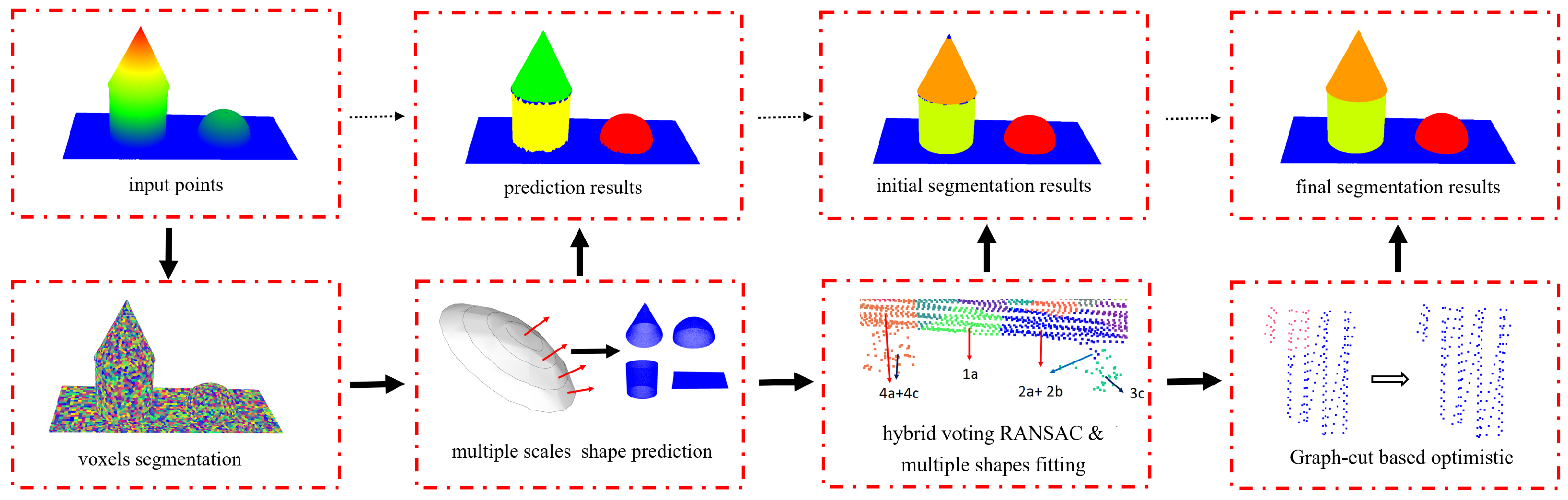
3.1. Overall Workflow and Problem Setup
3.1.1. Overall Workflow
3.1.2. Problem Setup
- 3D point P. Basic item, considering its position and normal vectors .
- Super voxel V. A group of points that have similar features and shape types. Each voxel has its centre of gravity and an average normal .
- Observation errors E. The consistency between the point and the proposed shapes, including the distance () and normal difference ().
- Shape type T. Each point or voxel needs to be classified into certain shape types, including planes, spheres, cylinders, and cones.
- Object segment S. A group of points and voxels with the same shape types and segment labels.
3.2. Multi-Scale Shape Prediction
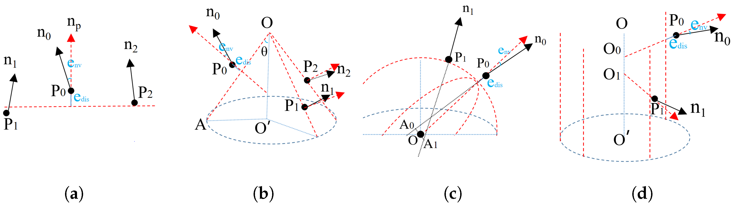
3.2.1. Shape Hypothesis
- Plane. A plane can be estimated using and other two random voxel centers, and .
- Cone. Two more samples, and , with normal vectors are used. Their apex O was intersected by the planes defined from the three point and normal pairs. The axis and the opening angle could from calculated by the average values of normalized , , and . Moreover, if we limit the axis to be vertical in some situations, one sample point will be sufficient.
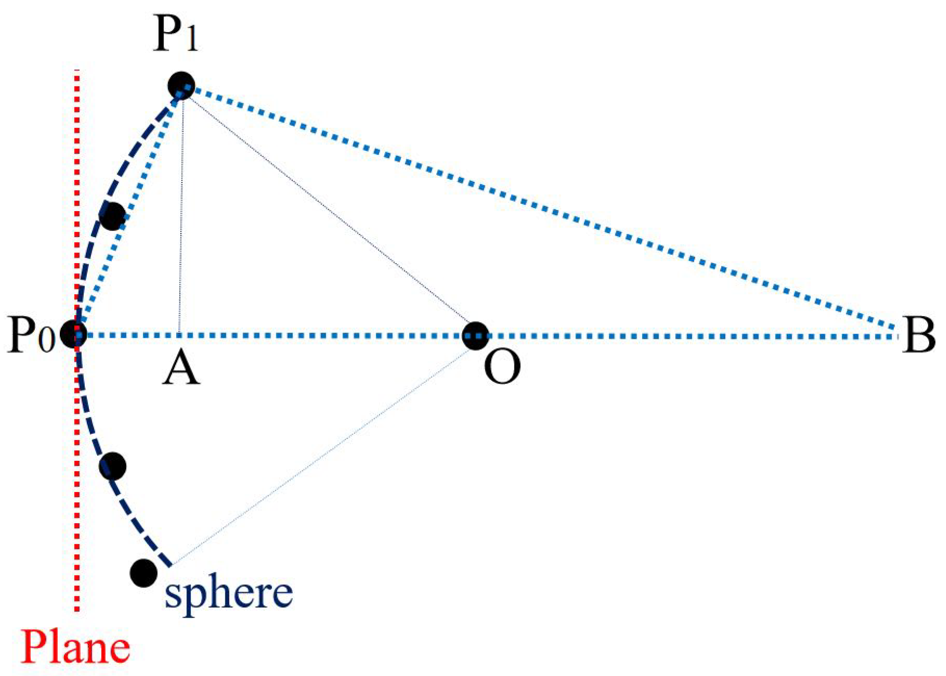
- Sphere. Another point with anormal vector is required. The sphere center O is the middle point of shortest line segment between the lines defined by the two point and normal pairs and . The sphere radius is the average of and .
- Cylinder. Another sample with a normal vector is sufficient. The axis orientation is defined by . We then project and to the plane vertically to the axis and intersect them for the center. The sphere radius is the average of and .
3.2.2. Shape Evaluation and Prediction
| Algorithm 1: Shape prediction |
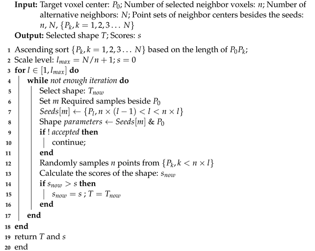 |
3.3. Hybrid Voting RANSAC-Based Segmentation
3.3.1. Hybrid Voting
3.3.2. Voxel-Based Connectivity
3.3.3. Post-Segmentation
3.4. Graph-Cut-Based Optimization
4. Experimental Evaluations
4.1. Dataset, Parameters, and Metrics
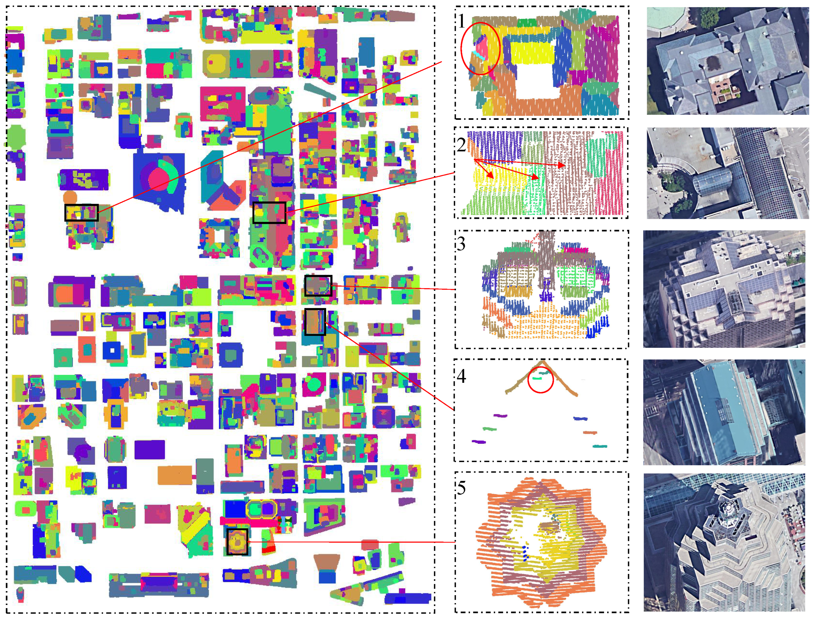
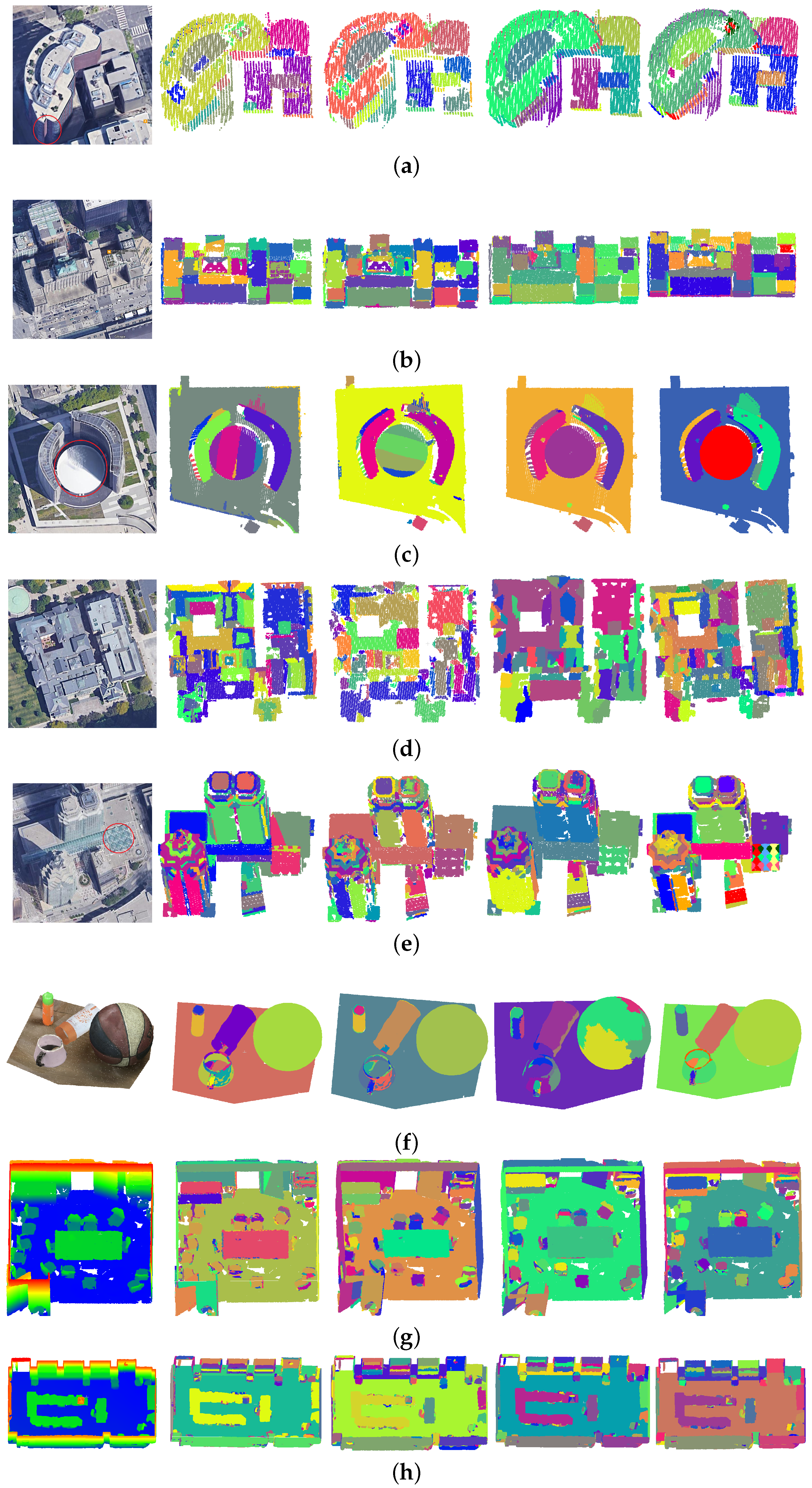
4.2. Overall Segmentation Results
4.3. Local Details and Precision
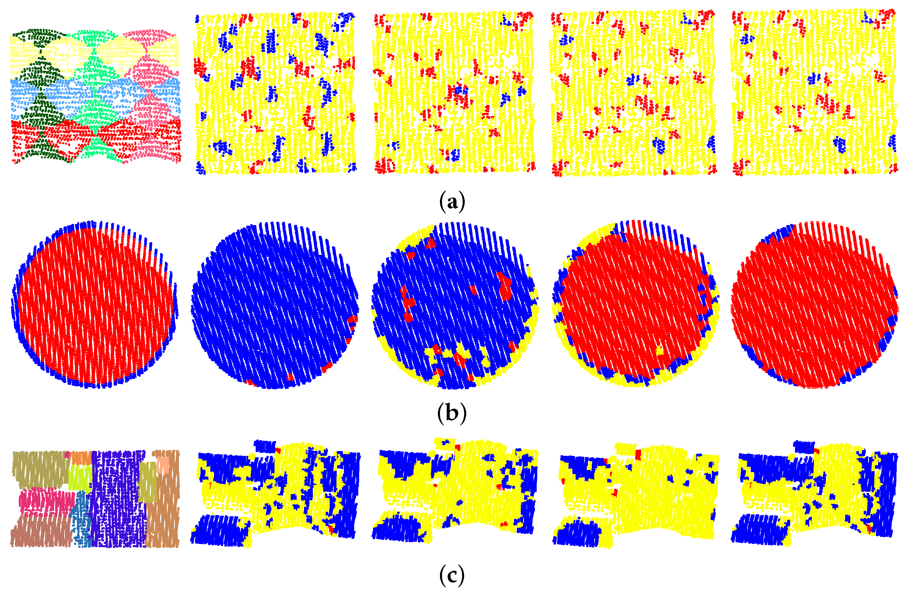
4.4. Parameter Sensitivity
4.5. Discussion
- Shape type competition. This issue is unavoidable in complex scenes or when the quality of data is poor. For instance, a horizontal plane may generate more inliers than the cylinders in Figure 8a, causing the poor results seen in Figure 9b. Considering that there are relatively fewer curved shapes, a prediction-then-segmentation strategy that estimates the shape type first is adopted. In Figure 8a, since most points are predicted as cylinders, the influence of other shapes and their meaningless iteration are avoided.
- Spurious shapes. Even if the shape types are successfully identified, spurious shapes will also cause trouble in current methods—i.e., the segmentation results obtained for efficient RANSAC shown in Figure 9c. A spurious plane can be accepted when it contains more inliers or the iteration terminates too early. In our work, the weighted RANSAC approach, which takes the point–shape distance and normal difference into consideration, is adopted. Spurious shapes with greater numbers of points but smaller total weights are suppressed. Moreover, the approaches adopted in post-segmentation and graph-cut-based optimization will also further improve the segmentation results.
- Object scale and neighborhood size. Since the shape prediction approach is achieved through local analysis, it can be influenced by neighborhood size. Meanwhile, when the radius of curved shapes is much larger than the neighborhood size, they can be identified as planes. As such, scale factors are considered in this work, including the radius of curved shapes and the neighborhood size. This ensures the extraction of multiple-scale curved shapes under various different scenes.
5. Conclusions
Author Contributions
Funding
Data Availability Statement
Acknowledgments
Conflicts of Interest
Abbreviations
| RANSAC | RANdom SAmple Consensus |
| MSAC | M-estimate SAmple Consensus |
| MLESAC | Maximum Likelihood-estimate SAmple Consensus |
References
- Haala, N.; Kada, M. An update on automatic 3D building reconstruction. ISPRS J. Photogramm. Remote Sens. 2010, 65, 570–580. [Google Scholar] [CrossRef]
- Musialski, P.; Wonka, P.; Aliaga, D.G.; Wimmer, M.; Van Gool, L.; Purgathofer, W. A survey of urban reconstruction. Comput. Graph. Forum 2013, 32, 146–177. [Google Scholar] [CrossRef]
- Zhu, L.; Lehtomäki, M.; Hyyppä, J.; Puttonen, E.; Krooks, A.; Hyyppä, H. Automated 3D Scene Reconstruction from Open Geospatial Data Sources: Airborne Laser Scanning and a 2D Topographic Database. Remote Sens. 2015, 7, 6710–6740. [Google Scholar] [CrossRef] [Green Version]
- Koelle, M.; Laupheimer, D.; Schmohl, S.; Haala, N.; Rottensteiner, F.; Wegner, J.; Ledoux, H. The Hessigheim 3D (H3D) benchmark on semantic segmentation of high-resolution 3D point clouds and textured meshes from UAV LiDAR and Multi-View-Stereo. ISPRS Open J. Photogramm. Remote Sens. 2021, 1, 100001. [Google Scholar] [CrossRef]
- Zhao, B.; Hua, X.; Yu, K.; Xuan, W.; Chen, X.; Tao, W. Indoor Point Cloud Segmentation Using Iterative Gaussian Mapping and Improved Model Fitting. IEEE Trans. Geosci. Remote Sens. 2020, 58, 7890–7907. [Google Scholar] [CrossRef]
- Shi, W.; Ahmed, W.; Li, N.; Fan, W.; Xiang, H.; Wang, M. Semantic Geometric Modelling of Unstructured Indoor Point Cloud. Int. J. Geo-Inf. 2018, 8, 9. [Google Scholar] [CrossRef] [Green Version]
- Schnabel, R.; Wahl, R.; Klein, R. Efficient RANSAC for Point-Cloud Shape Detection. Comput. Graph. Forum 2007, 26, 214–226. [Google Scholar] [CrossRef]
- Zhu, L.; Kukko, A.; Virtanen, J.-P.; Hyyppä, J.; Kaartinen, H.; Hyyppä, H.; Turppa, T. Multisource Point Clouds, Point Simplification and Surface Reconstruction. Remote Sens. 2019, 11, 2659. [Google Scholar] [CrossRef] [Green Version]
- Lin, Y.; Li, J.; Wang, C.; Chen, Z.; Wang, Z.; Li, J. Fast regularity-constrained plane fitting. ISPRS J. Photogramm. Remote Sens. 2020, 161, 208–217. [Google Scholar] [CrossRef]
- Tian, P.; Hua, X.; Yu, K.; Tao, W. Robust Segmentation of Building Planar Features From Unorganized Point Cloud. IEEE Access 2020, 8, 30873–30884. [Google Scholar] [CrossRef]
- Ying, S.; Xu, G.; Li, C.; Mao, Z. Point Cluster Analysis Using a 3D Voronoi Diagram with Applications in Point Cloud Segmentation. ISPRS Int. J. -Geo-Inf. 2015, 4, 1480–1499. [Google Scholar] [CrossRef]
- Serna, A.; Marcotegui, B.; Hernández, J. Segmentation of Facades from Urban 3D Point Clouds using Geometrical and Morphological Attribute-based Operators. ISPRS Int. J.-Geo-Inf. 2016, 5, 6. [Google Scholar] [CrossRef]
- Li, Y.; Ma, L.; Zhong, Z.; Cao, D.; Li, J. TGNet: Geometric Graph CNN on 3-D Point Cloud Segmentation. IEEE Trans. Geosci. Remote Sens. 2020, 58, 3588–3600. [Google Scholar] [CrossRef]
- Sampath, A.; Shan, J. Segmentation and Reconstruction of Polyhedral Building Roofs From Aerial Lidar Point Clouds. IEEE Trans. Geosci. Remote Sens. 2010, 48, 1554–1567. [Google Scholar] [CrossRef]
- Rabbani, T.; Heuvel, F.V.D.; Vosselman, G. Segmentation of point clouds using smoothness constraints. Int. Arch. Photogramm. Remote Sens. Spat. Inf. Sci. 2006, 36, 248–253. [Google Scholar]
- Luo, N.; Jiang, Y.; Wang, Q. Supervoxel Based Region Growing Segmentation for Point Cloud Data. Int. J. Pattern Recognit. Artif. Intell. 2020, 35, 2154007. [Google Scholar] [CrossRef]
- Wang, X.; Liu, S.; Shen, X.; Shen, C.; Jia, J. Associatively Segmenting Instances and Semantics in Point Clouds. arXiv 2019, arXiv:1902.09852. [Google Scholar]
- Zhao, L.; Tao, W. JSNet: Joint Instance and Semantic Segmentation of 3D Point Clouds. arXiv 2019, arXiv:1912.09654. [Google Scholar] [CrossRef]
- Xu, B.; Jiang, W.; Shan, J.; Zhang, J.; Li, L. Investigation on the Weighted RANSAC Approaches for Building Roof Plane Segmentation from LiDAR Point Clouds. Remote Sens. 2016, 8, 5. [Google Scholar] [CrossRef] [Green Version]
- Fischler, M.A.; Bolles, R.C. Random sample consensus: A paradigm for model fitting with applications to image analysis and automated cartography. Commun. ACM 1981, 24, 381–395. [Google Scholar] [CrossRef]
- Choi, S.; Kim, T.; Yu, W. Performance Evaluation of RANSAC Family. In Proceedings of the British Machine Vision Conference, London, UK, 7–10 September 2009; pp. 81.1–81.12. [Google Scholar]
- Chen, D.; Zhang, L.Q.; Li, J.; Liu, R. Urban building roof segmentation from airborne lidar point clouds. Int. J. Remote Sens. 2012, 33, 6497–6515. [Google Scholar] [CrossRef]
- Frederic, B.; Michel, R. Hybrid image segmentation using LiDAR 3D planar primitives. In Proceedings of the Workshop “Laser scanning 2005”, Enschede, The Netherlands, 12–14 September 2005. [Google Scholar]
- Awwad, T.M.; Zhu, Q.; Du, Z.; Zhang, Y. An improved segmentation approach for planar surfaces from unconstructed 3D point clouds. Photogramm. Rec. 2010, 25, 5–23. [Google Scholar] [CrossRef]
- Zeineldin, R.A.; El-Fishawy, N.A. FRANSAC: Fast RANdom Sample Consensus for 3D Plane Segmentation. Int. J. Comput. Appl. 2017, 167, 30–36. [Google Scholar]
- Papon, J.; Abramov, A.; Schoeler, M.; Wörgötter, F. Voxel Cloud Connectivity Segmentation-Supervoxels for Point Clouds. In Proceedings of the 2013 IEEE Conference on Computer Vision and Pattern Recognition, Portland, OR, USA, 23–28 June 2013; pp. 2027–2034. [Google Scholar]
- Torr, P.H.; Zisserman, A. MLESAC: A new robust estimator with application to estimating image geometry. Comput. Vis. Image Underst. 2000, 78, 138–156. [Google Scholar] [CrossRef] [Green Version]
- Berkhin, P. Survey of Clustering Data Mining Techniques; Springer: New York, NY, USA, 2006. [Google Scholar]
- Gallo, O.; Manduchi, R.; Rafii, A. CC-RANSAC: Fitting planes in the presence of multiple surfaces in range data. Pattern Recognit. Lett. 2011, 32, 403–410. [Google Scholar] [CrossRef] [Green Version]
- Lin, Y.; Wang, C.; Zhai, D.; Li, W.; Li, J. Toward better boundary preserved supervoxel segmentation for 3D point clouds. ISPRS J. Photogramm. Remote Sens. 2018, 143, 39–47. [Google Scholar] [CrossRef]
- Xu, Y.; Tong, X.; Stilla, U. Voxel-based representation of 3D point clouds: Methods, applications, and its potential use in the construction industry. Autom. Constr. 2021, 126, 103675. [Google Scholar] [CrossRef]
- Achanta, R.; Shaji, A.; Smith, K.; Lucchi, A.; Fua, P.; Süsstrunk, S. SLIC Superpixels Compared to State-of-the-Art Superpixel Methods. IEEE Trans. Pattern Anal. Mach. Intell. 2012, 34, 2274–2282. [Google Scholar] [CrossRef] [Green Version]
- Wang, N.; Chen, F.; Yu, B.; Wang, L. A Strategy of Parallel SLIC Superpixels for Handling Large-Scale Images over Apache Spark. Remote Sens. 2022, 14, 1568. [Google Scholar] [CrossRef]
- Comaniciu, D.; Meer, P. Mean shift: A robust approach toward feature space analysis. IEEE Trans. Pattern Anal. Mach. Intell. 2002, 24, 603–619. [Google Scholar] [CrossRef] [Green Version]
- Zhou, Y.; Ju, L.; Wang, S. Multiscale Superpixels and Supervoxels Based on Hierarchical Edge-Weighted Centroidal Voronoi Tessellation. IEEE Trans. Image Process. 2015, 24, 3834–3845. [Google Scholar] [CrossRef] [PubMed]
- Xu, Y.; Tuttas, S.; Hoegner, L.; Stilla, U. Geometric Primitive Extraction from Point Clouds of Construction Sites Using VGS. IEEE Geosci. Remote Sens. Lett. 2017, 14, 424–428. [Google Scholar] [CrossRef]
- Song, S.; Lee, H.; Jo, S. Boundary-enhanced supervoxel segmentation for sparse outdoor LiDAR data. Electron. Lett. 2014, 50, 1917–1919. [Google Scholar] [CrossRef] [Green Version]
- Shen, J.; Hu, M.; Yuan, B. A robust method for estimating the fundamental matrix. In Proceedings of the 6th International Conference on Signal Processing, Beijing, China, 26–30 August 2002; Volume 1, pp. 892–895. [Google Scholar]
- Moisan, L.; Moulon, P.; Monasse, P. Fundamental Matrix of a Stereo Pair, with A Contrario Elimination of Outliers. Image Process. Line 2016, 6, 89–113. [Google Scholar] [CrossRef] [Green Version]
- Su, Z.; Gao, Z.; Zhou, G.; Li, S.; Song, L.; Lu, X.; Kang, N. Building Plane Segmentation Based on Point Clouds. Remote Sens. 2021, 14, 95. [Google Scholar] [CrossRef]
- Li, L.; Yang, F.; Zhu, H.; Li, D.; Li, Y.; Tang, L. An improved RANSAC for 3D point cloud plane segmentation based on normal distribution transformation cells. Remote Sens. 2017, 9, 433. [Google Scholar] [CrossRef] [Green Version]
- Yan, J.X.; Shan, J.; Jiang, W.S. A global optimization approach to roof segmentation from airborne lidar point clouds. ISPRS J. Photogramm. Remote Sens. 2014, 94, 183–193. [Google Scholar] [CrossRef]
- Dong, Z.; Yang, B.; Hu, P.; Scherer, S. An efficient global energy optimization approach for robust 3D plane segmentation of point clouds. ISPRS J. Photogramm. Remote Sens. 2018, 137, 112–133. [Google Scholar] [CrossRef]
- Rottensteiner, F.; Sohn, G.; Gerke, M.; Wegner, J.D.; Breitkopf, U.; Jung, J. Results of the ISPRS benchmark on urban object detection and 3D building reconstruction. ISPRS J. Photogramm. Remote Sens. 2014, 93, 256–271. [Google Scholar] [CrossRef]
- Armeni, I.; Sax, S.; Zamir, A.R.; Savarese, S. Joint 2d-3d-semantic data for indoor scene understanding. arXiv 2017, arXiv:1702.01105. [Google Scholar]
- Awrangjeb, M.; Fraser, C.S. An Automatic and Threshold-Free Performance Evaluation System for Building Extraction Techniques From Airborne LIDAR Data. IEEE J. Sel. Top. Appl. Earth Obs. Remote Sens. 2014, 7, 4184–4198. [Google Scholar] [CrossRef]


| Method Type | 2D Clustering | 3D | |
|---|---|---|---|
| 3D Partitioning | Boundary Enhanced | ||
| Description | converts points into a 2D grid | uses octree or 3D cells | considers boundary quality |
| Pros and cons | fast, well researched, but only considers 2D information | voxels may overlap multiple planes | preserves boundaries |
| Examples | SLIC [32], Parallel SLIC [33], mean-shift [34], Multiscale Superpixels [35] | VCCS [26], VGS [36] | BESS [30,37] |
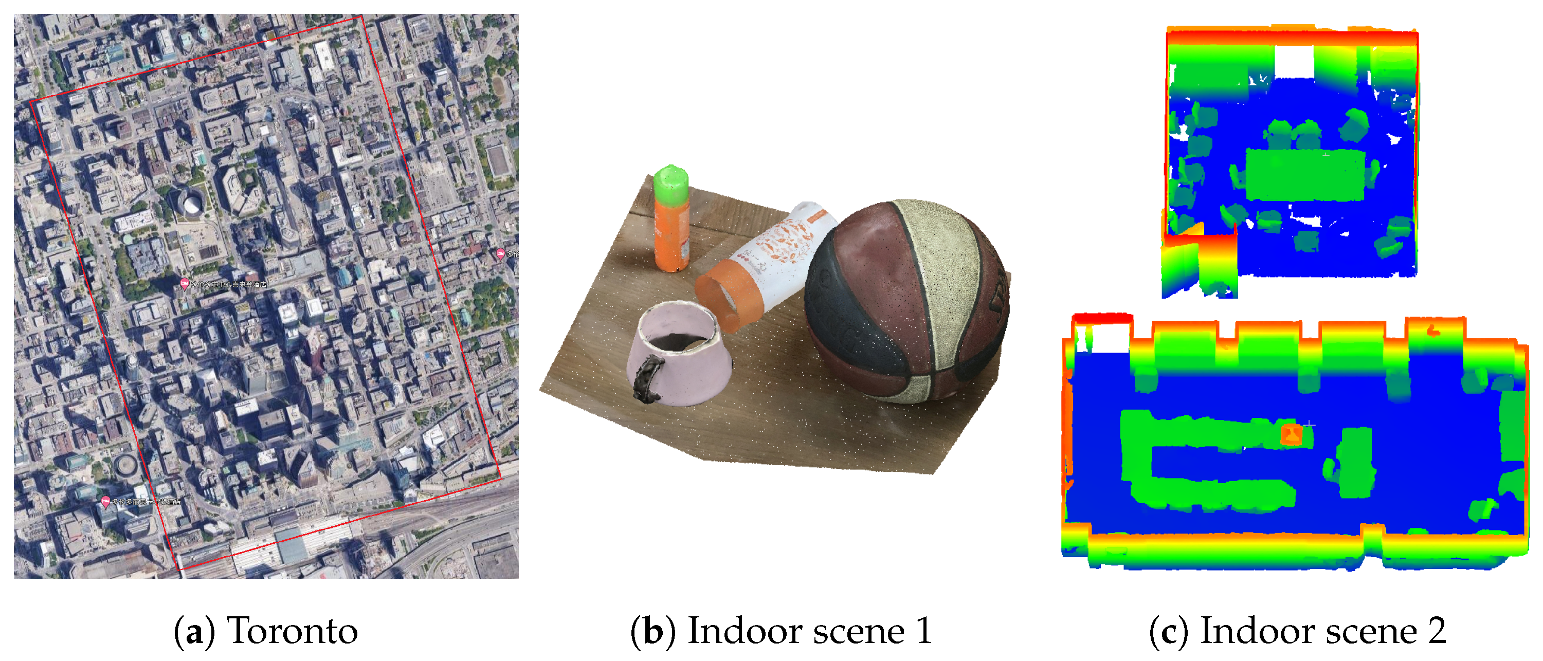
| Toronto | Indoor1 | Indoor2 | |
|---|---|---|---|
| Data | February 2009 | June 2021 | 2016 |
| System | ALTM-ORION M | Phone 8 plus | Matterport Camera |
| DOV | 650 m | 2–3 m | unknow |
| Density | ∼ | > | > |
| Voxel | Shape Prediction | RANSAC | ||||||||
|---|---|---|---|---|---|---|---|---|---|---|
| Toronto | 25 | 0.2 m | 10 | 2 m | 80% | 5 | 50 | 15 | 0.99 | 3 |
| Indoor 1 | 25 | 0.03 m | 10 | 0.05 m | 80% | 5 | 50 | 15 | 0.99 | 3 |
| Indoor 2 | 25 | 0.05 m | 10 | 0.1 m | 80% | 5 | 50 | 15 | 0.99 | 5 |
| ID | nPls | nCur | nTop | Meth | Segmentation | Curved Shapes | Topology | ||||||
|---|---|---|---|---|---|---|---|---|---|---|---|---|---|
| %cm | %cr | %qua | %cm | %cr | %qua | %cm | %cr | %qua | |||||
| a | 29 | 1 | 16 | eRAN | 83 | 92 | 77 | 100 | 50 | 50 | 69 | 85 | 61 |
| RG + eR | 93 | 87 | 82 | 100 | 50 | 50 | 81 | 93 | 76 | ||||
| GloL0 | 86 | 92 | 81 | / | / | / | 88 | 93 | 82 | ||||
| Ours | 93 | 93 | 87 | 100 | 100 | 100 | 94 | 88 | 83 | ||||
| b | 44 | 0 | 23 | eRAN | 86 | 86 | 76 | / | / | / | 83 | 86 | 73 |
| RG + eR | 98 | 81 | 78 | / | / | / | 96 | 81 | 76 | ||||
| GloL0 | 89 | 93 | 83 | / | / | / | 96 | 85 | 81 | ||||
| Ours | 93 | 91 | 85 | / | / | / | 87 | 91 | 80 | ||||
| c | 15 | 7 | 17 | eRAN | 80 | 60 | 52 | 57 | 36 | 29 | 47 | 58 | 32 |
| RG + eR | 80 | 57 | 50 | 57 | 36 | 29 | 47 | 58 | 32 | ||||
| GloL0 | 93 | 88 | 82 | / | / | / | 88 | 88 | 79 | ||||
| Ours | 100 | 88 | 88 | 100 | 78 | 78 | 100 | 81 | 81 | ||||
| d | 89 | 0 | 76 | eRAN | 73 | 89 | 67 | / | / | / | 45 | 79 | 40 |
| RG + eR | 75 | 79 | 63 | / | / | / | 42 | 64 | 34 | ||||
| GloL0 | 76 | 92 | 72 | / | / | / | 40 | 81 | 37 | ||||
| Ours | 88 | 93 | 82 | / | / | / | 83 | 93 | 78 | ||||
| e | 97 | 7 | 41 | eRAN | 77 | 87 | 69 | 0 | 0 | 0 | 54 | 81 | 48 |
| RG + eR | 73 | 83 | 58 | 0 | 0 | 0 | 49 | 87 | 45 | ||||
| GloL0 | 75 | 92 | 71 | / | / | / | 54 | 85 | 51 | ||||
| Ours | 92 | 86 | 80 | 100 | 100 | 100 | 88 | 92 | 82 | ||||
| f | 13 | 7 | 6 | eRAN | 92 | 75 | 71 | 100 | 78 | 78 | 100 | 88 | 88 |
| RG + eR | 92 | 75 | 71 | 100 | 78 | 78 | 100 | 88 | 88 | ||||
| GloL0 | 31 | 18 | 13 | / | / | / | 33 | 17 | 13 | ||||
| Ours | 92 | 92 | 86 | 100 | 88 | 88 | 100 | 100 | 100 | ||||
| g | 72 | 0 | 29 | eRAN | 70 | 85 | 63 | / | / | / | 90 | 87 | 79 |
| RG + eR | 75 | 79 | 63 | / | / | / | 90 | 93 | 84 | ||||
| GloL0 | 82 | 78 | 66 | / | / | / | 97 | 93 | 90 | ||||
| Ours | 85 | 87 | 75 | / | / | / | 97 | 93 | 90 | ||||
| h | 103 | 0 | 66 | eRAN | 77 | 79 | 65 | / | / | / | 91 | 88 | 81 |
| RG + eR | 84 | 76 | 67 | / | / | / | 89 | 91 | 82 | ||||
| GloL0 | 87 | 80 | 72 | / | / | / | 92 | 91 | 85 | ||||
| Ours | 86 | 83 | 73 | / | / | / | 94 | 89 | 84 | ||||
| sum | 462 | 22 | 274 | eRAN | 77 | 83 | 67 | 55 | 57 | 40 | 65 | 84 | 58 |
| RG + eR | 78 | 78 | 64 | 55 | 57 | 40 | 65 | 85 | 59 | ||||
| GloL0 | 81 | 84 | 70 | / | / | / | 68 | 84 | 60 | ||||
| Ours | 89 | 88 | 79 | 100 | 88 | 88 | 86 | 91 | 79 | ||||
Publisher’s Note: MDPI stays neutral with regard to jurisdictional claims in published maps and institutional affiliations. |
© 2022 by the authors. Licensee MDPI, Basel, Switzerland. This article is an open access article distributed under the terms and conditions of the Creative Commons Attribution (CC BY) license (https://creativecommons.org/licenses/by/4.0/).
Share and Cite
Xu, B.; Chen, Z.; Zhu, Q.; Ge, X.; Huang, S.; Zhang, Y.; Liu, T.; Wu, D. Geometrical Segmentation of Multi-Shape Point Clouds Based on Adaptive Shape Prediction and Hybrid Voting RANSAC. Remote Sens. 2022, 14, 2024. https://doi.org/10.3390/rs14092024
Xu B, Chen Z, Zhu Q, Ge X, Huang S, Zhang Y, Liu T, Wu D. Geometrical Segmentation of Multi-Shape Point Clouds Based on Adaptive Shape Prediction and Hybrid Voting RANSAC. Remote Sensing. 2022; 14(9):2024. https://doi.org/10.3390/rs14092024
Chicago/Turabian StyleXu, Bo, Zhen Chen, Qing Zhu, Xuming Ge, Shengzhi Huang, Yeting Zhang, Tianyang Liu, and Di Wu. 2022. "Geometrical Segmentation of Multi-Shape Point Clouds Based on Adaptive Shape Prediction and Hybrid Voting RANSAC" Remote Sensing 14, no. 9: 2024. https://doi.org/10.3390/rs14092024
APA StyleXu, B., Chen, Z., Zhu, Q., Ge, X., Huang, S., Zhang, Y., Liu, T., & Wu, D. (2022). Geometrical Segmentation of Multi-Shape Point Clouds Based on Adaptive Shape Prediction and Hybrid Voting RANSAC. Remote Sensing, 14(9), 2024. https://doi.org/10.3390/rs14092024