Article

Assessing the Performance of the Phase Difference Bathymetric Sonar Depth Uncertainty Prediction Model

1
Acoustics Group, Faculty of Aerospace Engineering, Delft University of Technology, 2629 HS Delft, The Netherlands
2
ITER Systems, 3 Rue du Lac Mont-Cenis, Batiment Est Supernova Savoie Technolac, 73290 La Motte-Servolex, France
*
Author to whom correspondence should be addressed.
Remote Sens. 2022, 14(9), 2011; https://doi.org/10.3390/rs14092011
Submission received: 8 April 2022 / Accepted: 19 April 2022 / Published: 22 April 2022

Abstract

:
Realistic predictions of the contribution of the uncertainty sources affecting the quality of the bathymetric measurements prior to a survey is of importance. To this end, models predicting these contributions have been developed. The objective of the present paper is to assess the performance of the bathymetric uncertainty prediction model for Phase Difference Bathymetric Sonars (PDBS) which is an interferometric sonar. Two data sets were acquired with the Bathyswath-2 system with a frequency of 234 k Hz at average water depths of around 26 m and 8 m with pulse lengths equal to 0.0555   m s and 0.1581   m s , respectively. The comparison between the bathymetric uncertainties derived from the measurements and those predicted using the current model indicates a relatively good agreement except for the across-track distances close to the nadir. The performance of the prediction model can be improved by modifying the term addressing the effect of footprint shift, i.e., spatial decorrelation, on the bottom due to fact that at a given time the footprints seen by different receiving arrays are slightly different.

Graphical Abstract

1. Introduction

Currently MultiBeam EchoSounder (MBES) systems are widely used for conducting bathymetric surveys [1,2,3]. They allow for efficient surveying of large areas and offer the possibility of complete bottom coverage. An MBES sends out an acoustic pulse along a wide swath perpendicular to the sailing direction. Beam steering at reception allows for determining the travel-time of the signal for a set of predefined beam angles [4]. For each ping, water depths along the swath are derived from the combination of travel times and beam angles, provided that the local Sound Speed Profile (SSP) in the water column is known [5].
However, surveys with MBES systems in shallow water are typically inefficient and thus costly due to the limited swath width. For an MBES system, data acquisition capability is typically limited to 3–5 times water depth. This does not pose a major limitation until working in waters shallower than 10 m–15 m where attaining a full bottom coverage becomes difficult. This has promoted the use of Phase Differencing Bathymetric Sonars (PDBS), also known as interferometric sonars, where the wide swath range of the sonar decreases the survey time and reduces the cost for a large survey area. PDBS use the phase difference of the backscattered signal at two closely spaced receivers for determining the Angle(s) of Arrival (AoA) [6].
Similar to any measurement system, PDBS measurements are affected by uncertainties. Thus, the derived depths are affected by uncertainties induced by the interferometer system, sound speed in the water column, and position, motion and attitude sensors. Obtaining a realistic a priori estimate of the depth uncertainties is of importance for a number of applications [7,8] including survey planning.
Over the past decades, approaches have been developed for the estimation of the bathymetric uncertainties. Regarding an MBES system, references [9,10] developed an a priori vertical uncertainty prediction model to quantify the contribution of various sources. The model has been improved by [11,12] to account for different types of transmitted pulse shapes and has been validated by [13] using measurements acquired for different environmental conditions and MBES settings. Reference [4] proposed a unified definition of a quality factor for sonar bathymetry measurements (both MBES and PDBS), which is an a posteriori estimator of the local depth uncertainty estimated based on the measured signal features. Reference [14] discusses the influence of the phase difference estimation uncertainties using a theoretical physic based framework of the backscattered signals. Different uncertainty sources inherent to the backscattered signal structure are considered and the performance of the developed model is assessed using various numerical simulations scenarios, see also [15] for quantification of the contribution of different sources. Reference [16] quantified the uncertainties discussed in [14] for the Bathyswath-2 system (manufactured by ITER Sytems) [17] which is a phase differencing system and addressed the effect of varying transmitted pulse length on the bathymetric uncertainties. The author did not account for the uncertainty sources induced by ancillary sensors and SSP in the water column. The objective of this contribution is to quantify the total PDBS bathymetric uncertainties accounting for different sources such as the interferometer, sound speed in the water column, motion and positioning sensors for a PDBS system and to compare the predictions to those encountered in reality. The contribution of this paper is thus to assess and validate the current available method for predicting the PDBS measured depth uncertainties. For the comparison use is made of the Bathyswath-2 system for different environmental conditions and sonar settings. This paper is organized as follows. In Section 2, a brief theory of interferometer systems is given followed by discussing the bathymetric uncertainties induced by the interferometer. Next, the approach taken for predicting total bathymetric uncertainty is briefly explained. The description of the data sets is given in Section 3. We present and discuss the results in Section 4. Concluding remarks are given in Section 5.

2. Interferometric Bathymetry Undertainty Prediction Model
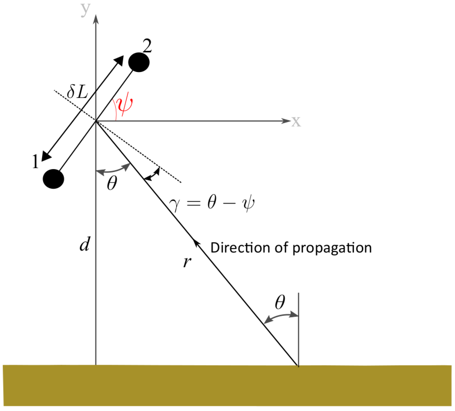
2.1. Interferometry

The interferometry principle is based on constructive and destructive interference between acoustic waves (or electromagnetic waves). Considering two waves from coherent sources, the resulting intensity depends on the phase difference between both waves [18]. Shown in Figure 1 is the geometry of angle and bathymetry measurements using interferometry. The angle ψ is the tilt angle relative to the x-axis and the angle θ is defined as the angle between the direction of propagation and the y-axis, i.e., depth axis (wavefront and x-axis). For an array made of two receivers equally distanced with δ L , the phase difference can be written as
Δ φ = 2 π λ δ r = 2 π λ δ L sin γ ,
with λ the acoustic wavelength equaling c f and f and c the frequency of the acoustic signal and sound speed respectively. γ = θ ψ is the angle between the direction of propagation and the interferometer axis. δ r is the difference in range from the source to the two receivers.
Thus, by measuring the phase difference, the angle of arrival can be determined. In practice, the phase difference Δ φ at a given time sample is estimated using an interferometric estimator based on the two complex signal envelopes received on the two array elements, s 1 and s 2 , as [19]
Δ φ ^ = arg ( s 1 s 2 * ) ,
with * the complex conjugate operator. The values given by the complex arg operator are between π , π . Thus, the relation between Δ φ and Δ φ ^ is Δ φ ^ = mod 2 π λ δ L sin γ , 2 π . A counter of phase rotations m ^ is thus introduced and Δ φ ^ is related to Δ φ as
Δ φ ^ ± 2 π m ^ = 2 π λ δ L sin γ m ^ N ,
with m ^ the integer phase ambiguity. The estimated phase difference thus becomes ambiguous and discontinuous, referred to as phase jumps. To address the phase ambiguity problem, occurring as soon as δ L (commonly referred to as the baseline length in interferometry) is larger than λ 2 , a number of approaches exist [20,21]. The widely used method for solving the phase ambiguity is the Vernier method [15,22]. The Vernier method does not require extra equipment or hardware change. The method requires at least three sensors (i.e., two receiver pairs) and creates artificial receiver pairs with a separation of λ 2 by subtracting the phase difference of two pairs [23,24]. For the Bathyswath system, four transducers are used at different spacings. For four transducers A, B, C and D, we can create an artificial λ 2 spacing by subtracting the AB phase difference from the BC phase difference, and thus an unambiguous but uncertain angle is obtained. With this unambiguous estimate of the angle, the uncertainty is decreased by choosing a larger element spacing. Repeating the process to increasingly larger pairs, gives a more certain estimate of the angle.

2.2. Bathymetry Uncertainty Prediction Model for PDBS Systems

In this subsection we will discuss the different sources of uncertainty affecting the bathymetric measurements obtained from the PDBS systems (interferometric systems). Except for the contribution of the interferometer, the uncertainty sources are similar to those for MBES system [10,13] and can be categorized as [25]
  • Interferometer contribution σ d Int ;
  • Angular motion sensor contribution, σ d AngMot , due to the uncertainties in roll and pitch measurements and imperfectness of their corrections;
  • Motion sensor and echosounder alignment contribution, σ d Align , due to the discrepancies between roll and pitch angle measurements at the motion sensor and the PDBS transducer;
  • Sound speed contribution, σ d SS , due to the sound speed uncertainties at the transducer array and those in the water column. In case of not using GNSS, a measurement of the height of the water surface relative to chart datum is needed (i.e., tide height);
  • Heave contribution, σ H , due to the uncertainties in the heave measurements and those induced due to the vertical motion of the transducer with respect to the vertical reference unit caused by the angular motions of the vessel. In case of using the Global Navigation Satellite System (GNSS) for vertical positioning, the uncertainty of the heave measurements is replaced by the uncertainty of the vertical component of the GNSS.
Assuming the above uncertainty sources are uncorrelated and have equal contribution to the final bathymetry uncertainty (this will be discussed later on in Section 4), the total depth uncertainty relative to the interferometer is expressed as
σ d = σ d Int 2 + σ d AngMot 2 + σ d Align 2 + σ d SS 2 + σ H 2
The equations for quantifying the contributions of σ d AngMot , σ d Align , σ d SS , σ H are not presented here and the interested reader can refer to [9,10]. Here, we briefly discuss the contribution of the interferometer, σ d Int . Before proceeding further, it should be highlighted that here we have considered the main uncertainty sources arising from the physics of the interaction of the acoustic environment and the measurement components and algorithms of the PDBS system. It is assumed that the sonar system has been designed such that internal sources of noise (and thus the corresponding bathymetry uncertainty) have been reduced to levels well below the contribution of the uncertainty sources mentioned above. For example, the front-end receiving pre-amplifiers are selected such that they have very low self-noise, and signal processing algorithms chosen do not add uncertainty to the processed data [26]. It is sometimes found that the electronic systems external to the sonar can introduce electrical noise which adds to the depth measurement uncertainty. System test procedures are available and to detect and address this issue. As an example, operating the system while the sonar transmit signal is turned off should provide an amplitude signal close to zero. Manufacturers often provide advice for solving any such problems.
A bathymetry measurement uncertainty induced by the interferometer is a combination of uncertainty in the time of arrival ( σ t ) and angle of arrival ( σ θ ) and is given as
σ d Int d = σ t t + σ θ tan θ
with t the two way travel time of the signal an d the depth below the PDBS transducer. Assuming that the time of arrival measurement is sufficiently accurate, the first term in Equation (5) can be neglected. This assumption is based on the high sampling frequency of the received signal.
The angular uncertainty ( σ θ ) is obtained from a differentiation of Equation (1), replacing γ by θ ψ as
σ θ = σ Δ φ 2 π λ δ L 1 cos ( θ ψ )
Angular measurement uncertainty is proportional to the phase difference uncertainty and is minimum for large values of δ L λ (a wide receiver spacing compared to signal wavelength), and cos ( θ ψ ) (a target close to the interferometer axis).
Substituting σ θ from Equation (6) in Equation (5) gives σ d Int as
σ d Int d = σ Δ φ 2 π λ δ L tan θ cos ( θ ψ )
Different uncertainty sources affect the phase difference uncertainty and thus the resulting bathymetry. The uncertainty of the phase measurements is approximated by [27]
σ Δ φ = 2 [ 12 π 2 + SNR ] 1 2 [ 1 0.05 SNR SNR + 1 ln SNR ] 1
with SNR the Signal-to-Noise Ratio of the received backscatter signal. Equation (8) provides an important relation between the SNR and the phase difference measurement uncertainty. Using Equation (8) in Equation (7), one can determine the bathymetric measurement uncertainty induced by the interferometer.
The uncertainty sources affecting the SNR may be either additive noise, or degradation related to the structure of the backscattered signal and are briefly described in the following subsection.

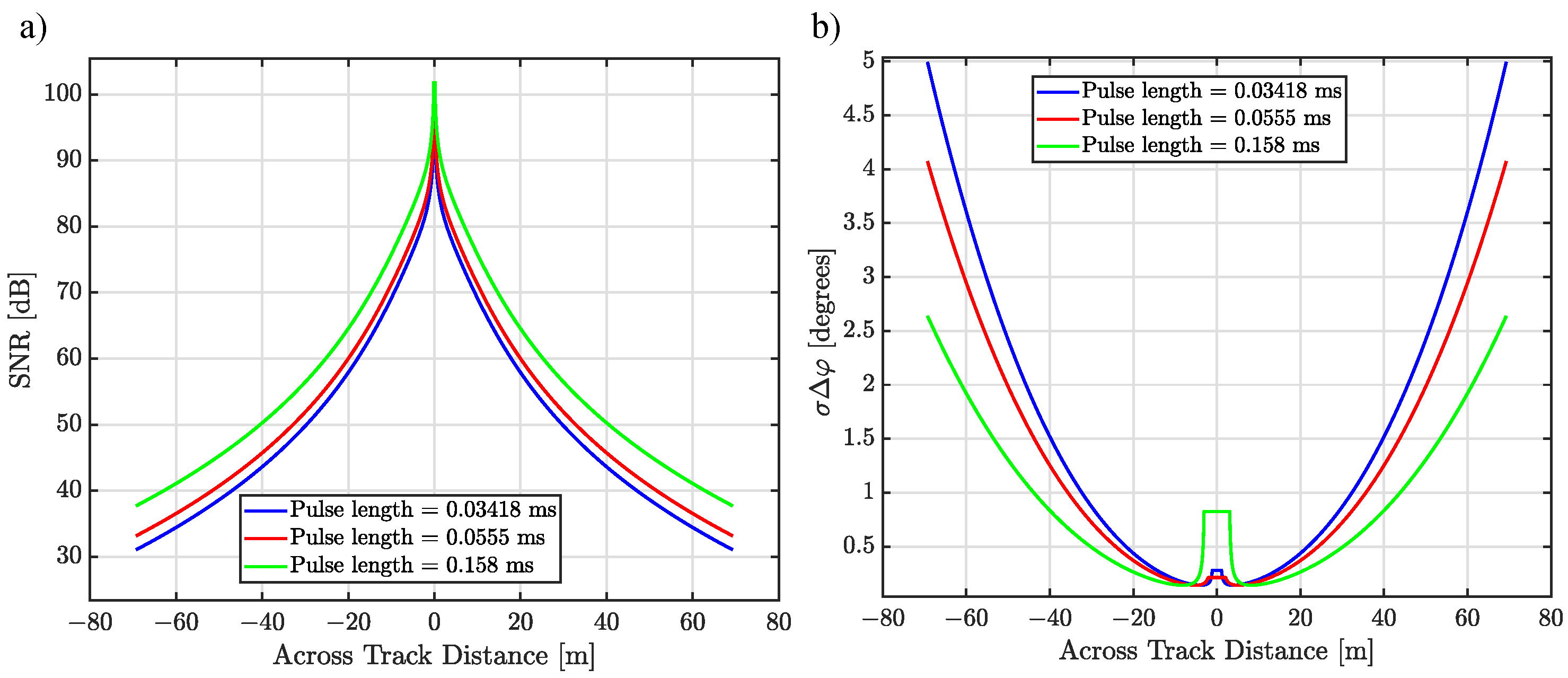
2.2.1. Additive Noise Contribution

Additive noise is a major limiting factor for interferometric sonars. Large additive noise can limit the attainable range and reduce the accuracy of angular measurements. Additive noise and its various causes can be assessed using the sonar equation [18,28]. In the calculation of the SNR due to the additive noise (referred to as SNR A d d ) information regarding the ambient noise ( N L 0 in Table 1), defined as any noise source present in the environment in the absence of the sonar, is required. Potential sources for this noise are sea-state (induced from the waves and wind), thermal (thermal agitation of the molecules of water producing pressure fluctuations at the face of the hydrophone), biological (from marine mammals and shrimps) and man-made (such as ships). Some of these sources can show impulsive nature instead of Gaussian [29]. This means that the performance of the signal processor designed assuming Gaussian noise, might be degraded in case of encountering impulsive noise. Studies have shown that at the high frequencies used by interferometric sonar systems (higher than 200 kHz), thermal noise is dominant [18,28,30] which does not show impulsive characteristic. Sea-state noise and ship noise are usually below the frequency of operation of the sonar, and are removed by band-pass filters.
Here we do not discuss the sonar equation, however we will use it to illustrate the effect of the pulse length on the SNR. In the sonar equation, the angular backscatter response is approximated by Lambert’s law [31]. This rule provides a specific incident angle dependency of the backscatter strength according to which many surfaces behave [28]. Figure 2 presents the evolution, with across-track distance, of the SNR and the corresponding phase difference uncertainty for three different pulse lengths (see Table 1). For the simulation, we use three different pulse lengths equal to 0.0342   m s , 0.0555   m s and 0.1580   m s which are representative of the frequently used pulse lengths in PDBS systems. As seen, using a longer pulse length results in higher SNR and consequently a smaller phase difference uncertainty.

2.2.2. Spatial Decorrelation Contribution

Ideally, the signals received on elements 1 and 2 in Figure 1 should only differ by their propagation range. Thus, theoretically their phase difference is only a function of the two path lengths at a given time, i.e., the two synchronous echoes should come from exactly the same scatterers [14,20,32].
However, at a given time, the footprints (instantly ensonified area) seen by different receiving arrays are slightly different. This difference depends on the receiver spacing ( δ L in Figure 1), depth d, incident angle θ and the transmitted pulse duration T (for a continuous wave signal shape) or equivalent duration after the pulse compression (for a frequency modulated signal shape). The phenomenon of receiving slightly different signals on the receiving elements is referred to as spatial decorrelation (sliding footprint) and contributes to the degradation of phase measurements due to a lower signal coherence (i.e., the degree of similarity between the two signals) [16].
The common part of the two individual footprints, referred to as the effective signal footprint, is used in the phase difference measurement. A Parasite contribution intervening as noise arises from the noncommon parts of the two individual footprints (which leads to decorrelation) [14]. The equivalent SNR is referred to as SNR S D and in linear scale (non dB values) is expressed as
SNR S D = c T δ L | sin γ | 1 .
The spatial decorrelation is penalizing for
  • A short continuous wave pulse or a short pulse compressed pulse duration for a frequency modulated signal;
  • Directions away from the interferometer axis; for the situation θ = ψ , SNR S D goes to infinity and the spatial decorrelation disappears;
  • A large interferometer spacing.
Shown in Figure 3a,b are the SNRs due to the spatial decorrelation ( SNR S D ) and the corresponding phase difference uncertainty, respectively. For the situation considered here with the interferometer tilt angle of 30 , the highest SNR (lowest phase difference uncertainty) occurs for the across-track distance of 17.35   m which corresponds to the across-track distance for the situation where θ = ψ . Similar to the additive noise contribution, one can see that an increase in the pulse length results in a higher SNR and smaller corresponding phase difference uncertainty.

2.2.3. Baseline Decorrelation Contribution

Signals arriving from scatterers located in the signal footprint overlap in time, i.e., the signals received at one instant of time result from contributions of all scatterers within the signal footprint. Hence, the footprint can be considered as a source dimension with its own directivity pattern [11]. This fluctuation and the fact that the two receivers observe the bottom along slightly different angular directions result in a decorrelation between the two received signals. This decorrelation is referred to as baseline decorrelation which is an intrinsic noise origin (i.e., inherent component of the acoustical signal) [4,14,33], and increases as the size of the footprint gets larger. The decorrelation process corresponds to an equivalent SNR, SNR B D , expressed as [14,32]
SNR B D = μ 1 μ
with μ the coherence coefficient which for a system transmitting a CW squared pulse is expressed as [27,32]
μ = sinc ( 2 π δ L λ d c T 4 cos θ cot θ cos γ )
with sinc ( x ) = sin x x the sinc function. Shown in Figure 4 is the SNR due to the baseline decorrelation and corresponding uncertainty of the phase measurements. For distances away from nadir, the SNR B D is usually high enough and has low impact on the phase measurements. This is due to the fact that the coherence between the received signals increases toward the outer part of the swath. For angles between nadir and the interferometry axis, the SNR B D is comparatively low.

2.2.4. Overal Signal-to-Noise Ratio

The final SNR should account for the contribution of additive noise (Section 2.2.1), spatial decorrelation (Section 2.2.2) and baseline decorrelation (Section 2.2.3). For now, we will only consider the degradation sources from the signal processing point of view, ignoring external factors impacting the measurement quality. These factors are denoted in Section 2.2 as σ d AngMot , σ d Align , σ d SS and σ H . Reference [27] proposes the following approach to account for different sources affecting SNR as
1 SNR T o t = G d ( 1 SNR A d d + 1 SNR S D + 1 SNR B D ) ,
where SNR T o t is the output SNR in linear units (non dB) due to the additive noise, baseline decorrelation and spatial decorrelation. G d is the array directivity index (array gain) [14,27]. The SNR due to the combined effect of additive noise (gray), spatial decorrelation (cyan) and baseline decorrelation (magenta) is shown with black in Figure 5a for a pulse length of 0.0555   m s . The corresponding phase measurement uncertainty is shown in Figure 5b.
The corresponding depth uncertainty due to SNR T o t is calculated substituting Equation (12) in Equation (8). σ Δ φ as obtained is then used in Equation (7) for the calculation of σ d Int .

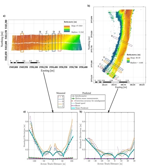
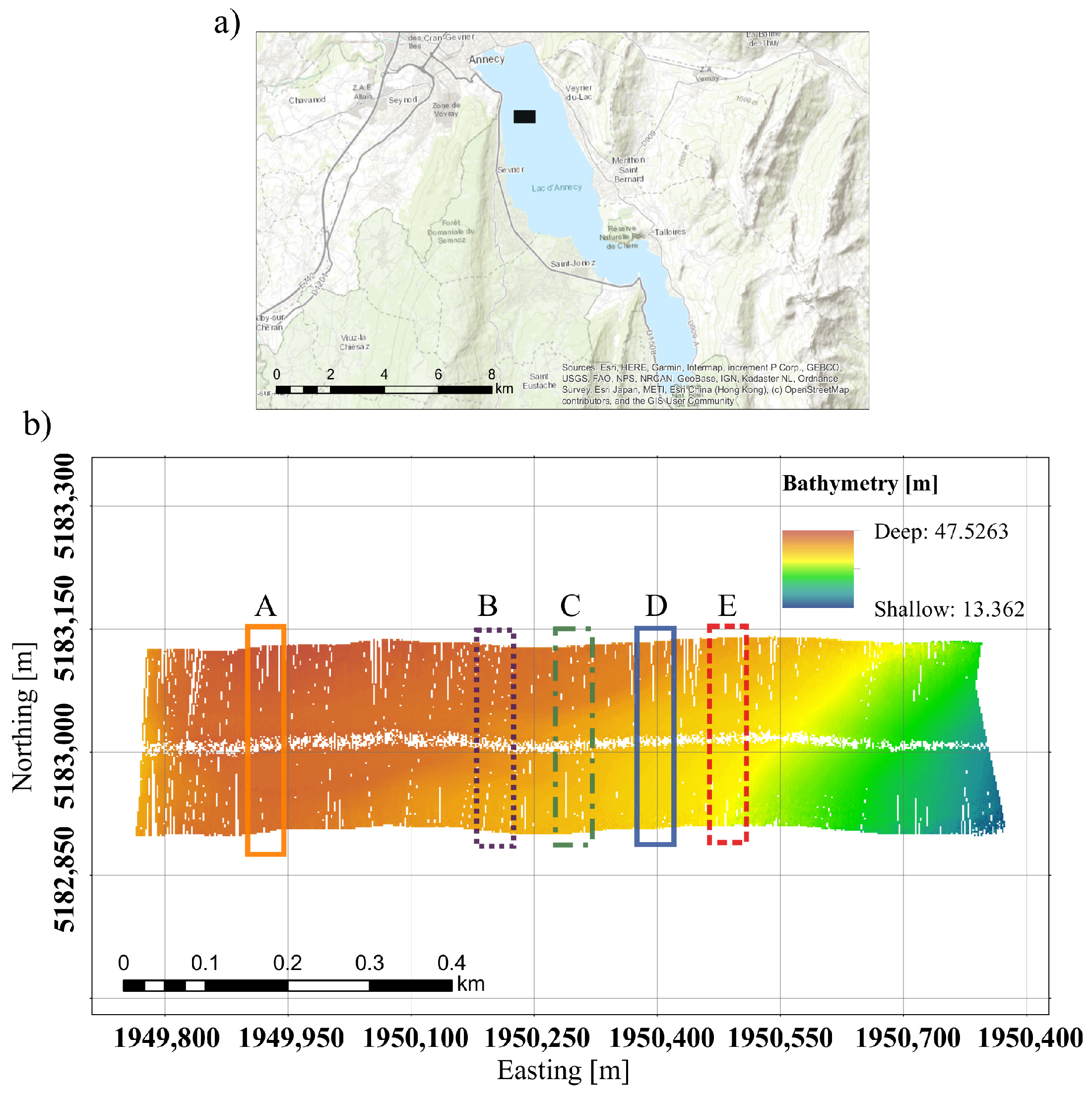
3. Description of the Data Sets

For validating the depth uncertainty model for the PDBS system, use is made of a Bathyswath-2 transducer, supplied by ITER Systems on a fixed platform with minimal motion.
A critical element for accurate estimation of the depth below the transducer is the Sound Speed Profile (SSP) in the water column which varies both spatially and temporally. Therefore, sufficient and accurate measurements of SSPs are required. To ensure the former a new SSP was taken in case of a difference of more than 2 m / s between the surface sound speed value and the sound speed from the latest full SSP [34]. The sound velocity profiler (miniSVP) was manufactured by Valeport and the uncertainty of its measurements as indicated by the manufacturer in a laboratory is 0.02   m / s [35]. However, from measurements at different locations (The Ministry of Infrastructure and Water Management of the Netherlands (Rijkswaterstaat) took 10 SSP measurements at 10 different location in inland waterways and the North Sea), the practical uncertainty was found to be 0.2   m / s , and hence this value was chosen as a practical value for the description of the system’s uncertainty and is used to quantify the resulting depth uncertainty.
The data sets were acquired using the “Swath Processor” (developed by ITER Systems) and GNSS sensors received the correction signal from Real-time Kinematic (RTK) services. GNSS RTK provides accurate position and ellipsoidal height of the GNSS antenna with an accuracy of a few centimeters in the WGS84 reference frame. The seafloor depth relative to the chart is then derived using the ellipsoidal height, GNSS antenna and transducer offsets from the vessel’s center of gravity (COG) and chart datum shift, obtained from chart datum models, an example of this is given in [36,37]. Thus, the uncertainty induced by the chart datum has been already included in the vertical positioning uncertainty, and hence there is no need to add this as a separate contributor to the total bathymetry uncertainty. Using GNSS for calculating the bathymetry implies that accounting for height offsets, such as dynamic draft, height above draft reference and tide, is not necessary for the depth calculation. Heave measurements are used within the processing software to calculate the height of the vessel’s center of gravity between two position updates (because the sonar system and Inertial Navigation Sensor (INS) have higher update rate than many GNSS system) [38]. Therefore, the accuracy of heave measurements acquired by the INS contributes to the uncertainty in the estimate of the depth. Ekinox-E manufactured by SBG Systems [39] was used for providing position, true heading, attitude, speed, and heave. The roll and pitch uncertainties of the system with RTK aiding are 0.02 (similarly the misalignment uncertainties are assumed to be 0.02 ).
Two areas with different bottom morphology, bathymetry and sonar settings were considered. The surveys were carried out in Annecy Lake, France (Figure 6), and Gomti River, India (Figure 7). Annecy Lake is a lake in Haute-Savoie region in France and is the second largest lake in France. The sound speed in the water column was varying between 1434.17   m / s and 1491.42   m / s with the average value of 1463.07   m / s . The Gomti River is an alluvial river of the Ganga Plain and is one of the important tributaries of the Ganga, originating near Mainkot, from Fulhar Jheel (also known as Gomat Taal) Lake in Madhotanda. The survey was carried out 30 k m from the city of Lucknow. The constant sound speed of 1489 m / s was used for this survey.
For both surveyed areas, the centre frequency of transducer was 234 k Hz with around 100 k Hz bandwidth. A complete Bathyswath-2 interferometric system consists of a dual transducer set looking to both port and starboard sides [17] with a tilt angle equaling 30 . For the data sets acquired in the Annecy Lake and Gomti River the pulse lengths were 0.0555   m s and 0.1581   m s , respectively. The other sonar related parameters are presented in Table 1.
It should be noted that we take the approach presented in [13] to account for the effect of potential along- and across-track slopes. However, the bottom morphology might change from one patch to another. Therefore, it is decided to consider small areas consisting of a number of patches (5 areas indicated as A, B, C, D and E with different colors in Figure 6 and Figure 7), i.e., not the full survey area, to minimize the variations of the bottom morphology when calculating the measured bathymetric uncertainties. In the present contribution it is assumed that the effect of potentially remaining small-scale bathymetry variations can be neglected in the modeling.

4. Results and Discussion

The size of the surface patch on the bottom is of importance. If a too large surface patch is considered, the variations of the measured uncertainties within a patch cannot be solely associated to the PDBS as the small-scale roughness affects the vertical uncertainties. On the other hand, if a too small patch is considered, the number of measurements within a patch is not enough for a robust estimate of the uncertainty [13]. We thus considered the patch size of 7 pings in the along-track direction by 0.5   m in the across-track direction. The minimum (sufficient) number of measurements within a patch for the estimation of the slopes and the uncertainties depends on various parameters such as water depth and beam angle. For the two surveys considered here, this number was assumed to be 10. For the deepest part of the data set acquired in Annecy Lake and Gomti River and the most outer beam, the Two-way Travel Time (TWTT) equals 0.17   s and 0.06   s respectively (i.e., ping rates of 6 Hz and 16 Hz ). Therefore, 7 pings in the along-track direction with the survey speed of 4.11   m / s correspond to 4.84   m and 1.77   m for the Annecy Lake and Gomti River surveys respectively.
The calculation of the measured bathymetric uncertainties was carried out by fitting a bi-quadratic or planar function (in 2 directions) to the measurements within each surface patch. The degree of the fit function (linear or bi-quadratic) was chosen based on the curvature, which is a measure of the surface patch deviation from a flat plane. For a surface patch with a curvature smaller than 0.5 / m a linear function was used for the fit, otherwise a bi-quadratic fit was employed.

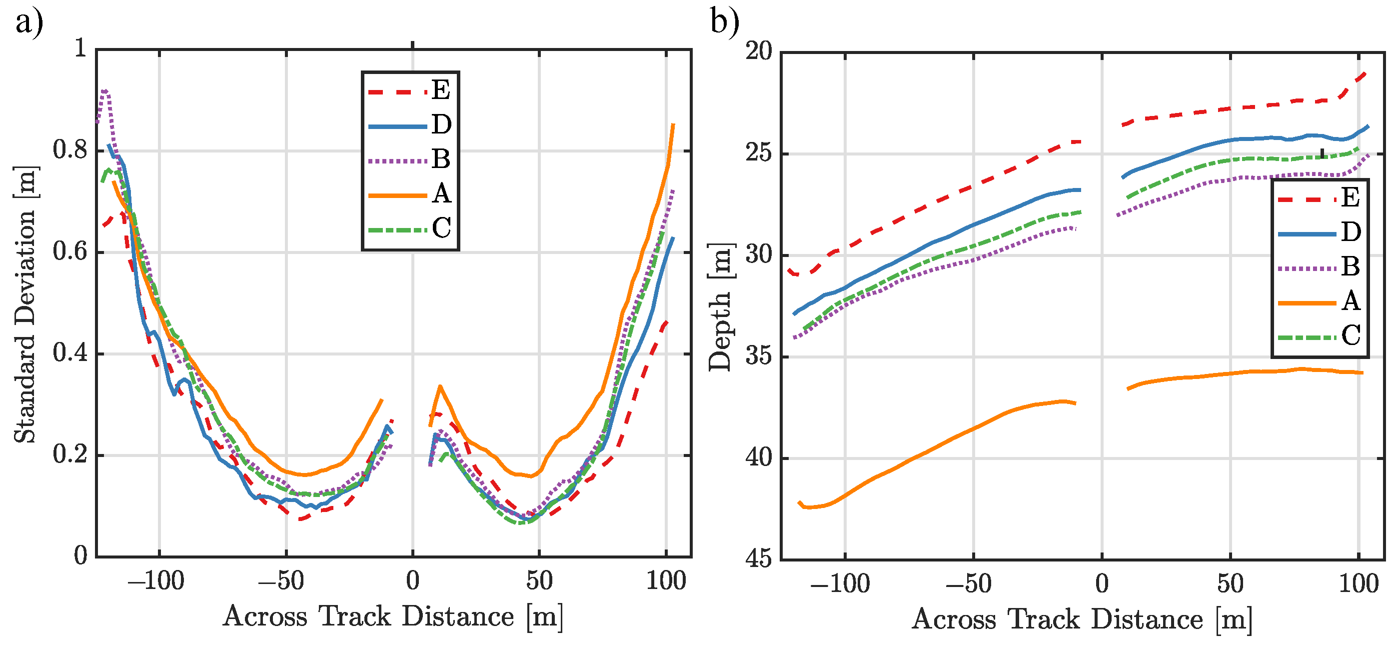
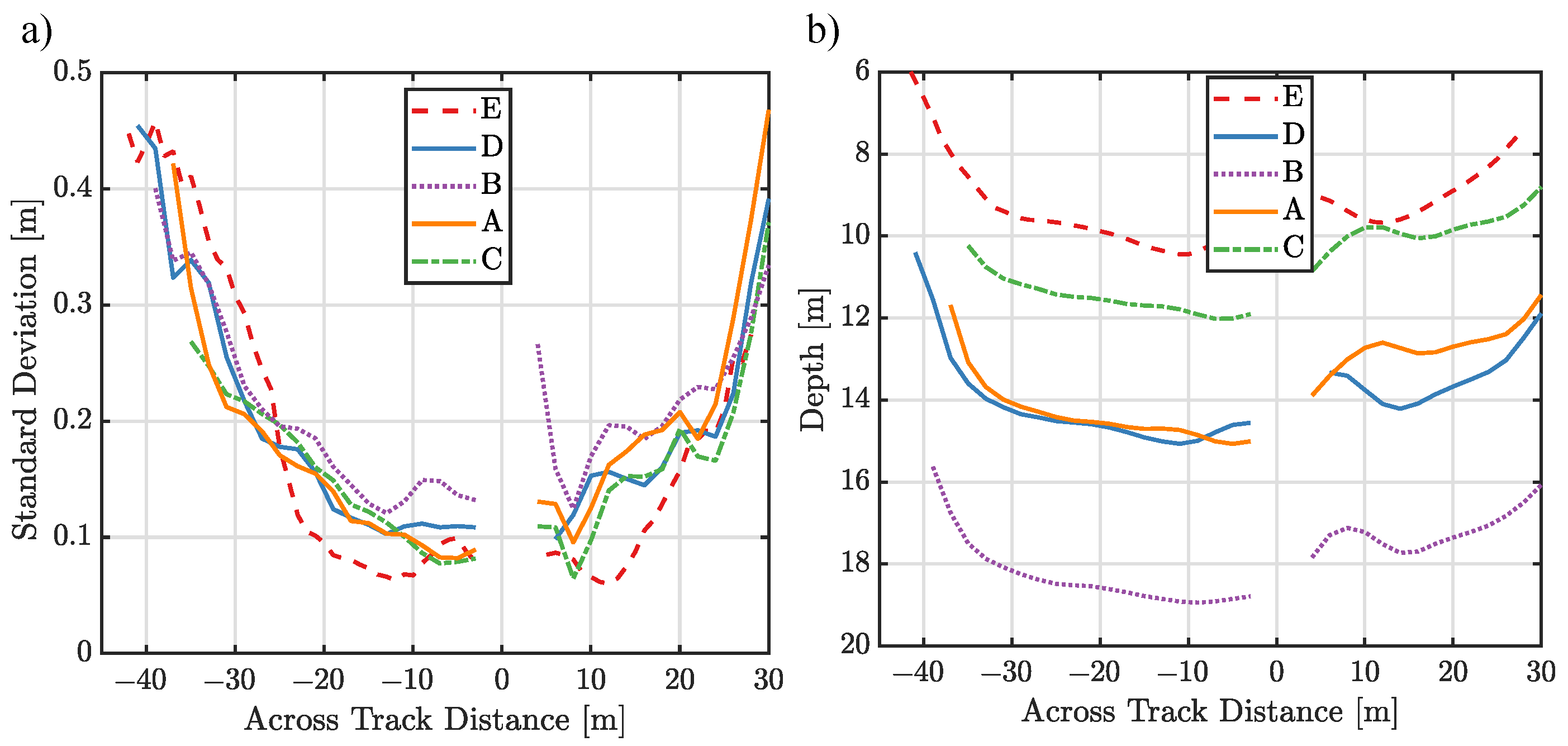
4.1. Trends Visible in Measured Bathymetric Uncertainties

Before comparing the modelled and measured uncertainties, the latter as obtained from the measurement with varying pulse lengths and environmental conditions is presented in Figure 8a and Figure 9a for Annecy Lake and Gomti River, respectively. Shown in Figure 8b and Figure 9b are the corresponding bathymetry profiles. Different colors correspond to the five different areas indicated as A, B, C, D and E in Figure 6 and Figure 7 to provide a better understanding of the variations of the morphology and uncertainty over the surveyed areas. For the shallower surveyed area, Figure 9, the swath width on the starboard side is smaller than that of the port due to limitations by the riverbank. The comparison between bathymetric uncertainties for the two areas indicates that for the deeper area, Figure 8, larger uncertainties are derived by a factor of around 1.7, in agreement with [13]. The authors showed that increasing the water depth from 10 m to 30 m without changing the pulse length resulted in an increase in the MBES bathymetric uncertainties by a factor of around 2.5 [13]. We intuitively expected to see such an increase in the bathymetric uncertainties for the measurements acquired with PDBS system. However, the smaller increase observed can be explained by a smaller pulse length used in Annecy Lake compared to that of Gomti River. In Figure 8, for the across-track distances close to nadir the bathymetric uncertainties are around 0.30   m . As the across-track distance increases, the bathymetric uncertainty decreases and reaches its minimum at around 50 m across-track distance. Larger bathymetric uncertainties close to nadir followed by a decrease also holds for Figure 9 (for a smaller portion of the swath compared to Figure 8).

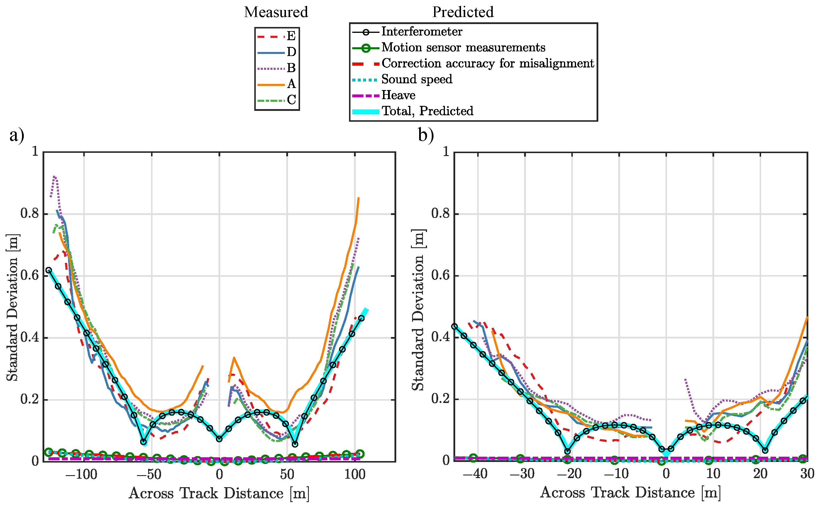
4.2. Comparing Modelled and Measured Uncertainties

The modelled bathymetric uncertainties are determined using the characteristics of the PDBS and its setting during the data acquisition (see Table 1), uncertainties of the sound speed measurements and motion sensors, environmental and survey related parameters (such as the average depth, transducer draft and vessel speed). It should be highlighted that the uncertainty predictions presented here are for this special situation and are not to be viewed as the uncertainty predictions applicable to a different scenario.
Shown in Figure 10a,b are the modelled and measured bathymetric uncertainties for the areas indicated as A, B, C, D and E with rectangles with varying colors in Figure 6 and Figure 7 respectively. Both the measured and predicted uncertainties increase with increasing depth. As mentioned in Section 2.2, the total predicted uncertainty (Equation (4)) assumes equal contribution of all factors which might not be a valid assumption. As an example, the contribution of the beam opening angle largely depends on the bottom morphology. This means that while for the flat bottom might overestimate the uncertainties, for a bottom with morphology probably underestimation of the uncertainties occurs. Including weight factors to capture phenomena which have not been taken into account in the model can be advantageous and can improve the agreement between the model predictions and measurements. This has not been considered in the present paper and can be a topic for further research.
In general, the uncertainties derived from the prediction model are in a good agreement with those encountered in reality with larger discrepancies for the beams close to nadir for the data set acquired in the Annecy Lake. The measured bathymetric uncertainty increases for the outer parts of the swath which is captured by the prediction model.
As can be seen, the most dominant source of uncertainty is predicted to be the interferometer contribution (black circle marker) contribution. As discussed in Section 2.2.1, Section 2.2.2 and Section 2.2.3 this contribution is composed of three parts, i.e., additive noise, spatial decorrelation and baseline decorrelation. The contribution of the motion sensor measurements, correction accuracy for misalignment, sound speed and heave is negligible and thus the total bathymetric uncertainty almost coincides with the uncertainty induced by the interferometer system. For the distances close to nadir, where the largest discrepancies occur, the most dominant error source is the spatial decorrelation. Comparing the measured and predicted uncertainties suggests that this term requires modification.

5. Conclusions

Predicting the uncertainty of PDBS bathymetric measurements is an important and almost standard step in the planning of a survey. Models have been developed to fulfill such a purpose enabling one to assess whether the required survey standards can be met in a specific measurement campaign for a given combination of measurement equipment, PDBS and environmental settings.
This paper has focused on assessing the performance of a PDBS bathymetric uncertainty prediction model. To this end, the predicted uncertainties are compared to those measured using different pulse lengths and water depths. To obtain the measured bathymetric uncertainties such that a fair comparison can be made with those modelled, areas with minimum variation in the water depth are selected. The potential remaining small scale variation in the bathymetry has been taken into account by fitting either a linear or bi-quadratic function (depending on the curvature) to the measurements within a surface patch of size 7 pings in the along-track direction (corresponding to 4.84   m and, 1.77   m for the Annecy Lake and Gomti River surveys respectively) by 0.5   m in the across-track direction.
Regarding the measured bathymetric uncertainties, it is seen that an increase in the bathymetry (from Gomti River to Annecy Lake) results in an increase in the corresponding uncertainties. However, with such an increase in depth, one would expect a larger increase in bathymetric uncertainties. This discrepancy can be explained by the fact that as a shorter pulse length was used for the data set in Annecy Lake (deeper part), where the increase in the uncertainty is partly compensated.
In general, the magnitude of the bathymetric uncertainties derived from the uncertainty prediction model are in good agreement with those measured. However, discrepancies have been observed for across-track distances close to nadir with the model underestimating the measured uncertainties. For this part of the swath, the most dominant uncertainty source is the spatial decorrelation. Thus, modification of this term to reflect the impact of receiving different signals on the receiving elements in a more realistic manner will improve the agreements between the predicted and measured uncertainties. Additionally, the performance of the model might be improved by including weight factors for phenomena which have not been accounted for in the uncertainty prediction model.

Author Contributions

Conceptualization, T.H.M.; methodology, T.H.M., M.G. and J.S.S.; software, T.H.M., M.G. and J.S.S.; validation, T.H.M.; formal analysis, T.H.M., M.G. and J.S.S.; investigation, T.H.M., M.G. and J.S.S.; resources, M.G. and J.S.S.; data curation, T.H.M.; writing—original draft preparation, T.H.M.; writing—review and editing, T.H.M., M.G., J.S.S., M.S. and D.G.S.; visualization, T.H.M.; supervision, M.S. and D.G.S.; project administration, M.S. and D.G.S.; funding acquisition, M.S. and D.G.S. All authors have read and agreed to the published version of the manuscript.

Funding

This investigation is part of a Postdoctoral research, funded by Ministry of Infrastructure of the Netherlands (Rijkswaterstaat).

Conflicts of Interest

J.S.S. and M.G. are employees and shareholders of ITER Systems SARL. The risk of their potential conflict of interest was mitigated by full editorial control of the first author. There was no attempt from J.S.S. and M.G. to influence the content of the paper or to influence the reputation of the products of ITER Systems. No benefits, financial or otherwise, were provided or promised by ITER Systems to the other authors of the paper. The findings of the paper apply equally to all interferometric sonar systems, which includes the competitors of ITER Systems. The addition of interferometric sonar data quality analysis to is beneficial to all manufacturers and users of interferometric sonar systems. T.H.M., M.S. and D.G.S. declare no conflict of interest.

References

  1. Anderson, T.J.; Syms, C.; Roberts, D.A.; Howard, D.F. Multi-scale fish-habitat associations and the use of habitat surrogates to predict the organisation and abundance of deep-water fish assemblages. J. Exp. Mar. Biol. Ecol. 2009, 379, 34–42. [Google Scholar] [CrossRef]
  2. Komatsu, T.; Igarashi, C.; Tatsukawa, K.; Sultana, S.; Matsuoka, Y.; Harada, S. Use of multi-beam sonar to map seagrass beds in Otsuchi Bay on the Sanriku Coast of Japan. Aquat. Living Resour. 2003, 16, 223–230. [Google Scholar] [CrossRef]
  3. Di Maida, G.; Tomasello, A.; Luzzu, F.; Scannavino, A.; Pirrotta, M.; Orestano, C.; Calvo, S. Discriminating between Posidonia oceanica meadows and sand substratum using multibeam sonar. ICES J. Mar. Sci. 2011, 68, 12–19. [Google Scholar] [CrossRef] [Green Version]
  4. Lurton, X.; Augustin, J.M. A measurement quality factor for swath bathymetry sounders. IEEE J. Ocean. Eng. 2010, 35, 852–862. [Google Scholar] [CrossRef]
  5. Hellequin, L.; Boucher, J.M.; Lurton, X. Processing of high-frequency multibeam echo sounder data for seafloor characterization. IEEE J. Ocean. Eng. 2003, 28, 78–89. [Google Scholar] [CrossRef] [Green Version]
  6. Pryor, D. Theory and test of bathymetric side scan sonar. In Proceedings of the OCEANS ’88, ’A Partnership of Marine Interests’ Proceedings, Baltimore, MD, USA, 31 October–2 November 1988; Volume 2, pp. 379–384. [Google Scholar]
  7. Eakins, B.W.; Taylor, L.A. Seamlessly integrating bathymetric and topographic data to support tsunami modeling and forecasting efforts. In Ocean Globe; Breman, J., Ed.; Esri Press: Redlands, CA, USA, 2010; Chapter 2; pp. 37–56. [Google Scholar]
  8. Hare, R.; Eakins, B.W.; Amante, C.; Taylor, L.A. Modeling bathymetric uncertainty. Int. Hydrogr. Rev. 2011, 6, 31–42. [Google Scholar]
  9. Hare, R. Depth and position error budgets for multibeam echosounding. Int. Hydrogr. Rev. 1995, LXXII, 37–69. [Google Scholar]
  10. Hare, R. Error Budget Analysis for US Naval Oceanographic Office (NAVOCEANO) Hydrographic Survey Systems; Technical Report; Hydrographic Science Research Center (HSRC): Mississippi, MS, USA, 2001. [Google Scholar]
  11. Mohammadloo, T.H.; Snellen, M.; Simons, D.G. Multi-beam echo-sounder bathymetric measurements: Implications of using frequency modulated pulses. J. Acoust. Soc. Am. 2018, 144, 842–860. [Google Scholar] [CrossRef] [PubMed] [Green Version]
  12. Mohammadloo, T.H.; Snellen, M.; Amiri-Simkooei, A.; Simons, D.G. Comparing modeled and measured bathymetric uncertainties: Effect of Doppler and baseline decorrelation. In Proceedings of the OCEANS 2019, Marseille, France, 17–20 June 2019; pp. 1–8. [Google Scholar]
  13. Mohammadloo, T.H.; Snellen, M.; Simons, D.G. Assessing the Performance of the Multi-Beam Echo-Sounder Bathymetric Uncertainty Prediction Model. Appl. Sci. 2020, 10, 4671. [Google Scholar] [CrossRef]
  14. Lurton, X. Swath bathymetry using phase difference: Theoretical analysis of acoustical measurement precision. IEEE J. Ocean. Eng. 2000, 25, 351–363. [Google Scholar] [CrossRef]
  15. Grall, P.; Kochanska, I.; Marszal, J. Direction-of-Arrival Estimation Methods in Interferometric Echo Sounding. Sensors 2020, 20, 3556. [Google Scholar] [CrossRef] [PubMed]
  16. Sewada, J.S. Contribution to the Development of Wideband Signal Processing Techniques for New Sonar Technologies. Ph.D. Thesis, Université Grenoble Alpes, Grenoble, France, 2020. [Google Scholar]
  17. ITER Systems. Bathyswath-2 Technical Information; Technical Report; ITER Systems: Auvergne-Rhone-Alpes, France, 2020. [Google Scholar]
  18. Lurton, X. An Introduction to Underwater Acoustics: Principles and Applications, 2nd ed.; Springer: Berlin/Heidelberg, Germany, 2010. [Google Scholar]
  19. Burdic, W.S. Underwater Acoustic System Analysis, 2nd ed.; Prentice-Hall: Englewood Cliffs, NJ, USA, 1991. [Google Scholar]
  20. Denbigh, P.N. Swath bathymetry: Principles of operation and an analysis of errors. IEEE J. Ocean. Eng. 1989, 14, 289–298. [Google Scholar] [CrossRef]
  21. Denbigh, P.N. Signal processing strategies for a bathymetric sidescan sonar. IEEE J. Ocean. Eng. 1994, 19, 382–390. [Google Scholar] [CrossRef]
  22. Sintes, C.; Solaiman, B. Strategies for unwrapping multisensors interferometric side scan sonar phase. In Proceedings of the OCEANS 2000 MTS/IEEE Conference and Exhibition. Conference Proceedings (Cat. No.00CH37158), Providence, RI, USA, 11–14 September 2000; Volume 3, pp. 2059–2065. [Google Scholar]
  23. Llort-Pujol, G.; Sintes, C.; Gueriot, D. Analysis of Vernier interferometers for sonar bathymetry. In Proceedings of the OCEANS 2008, Quebec City, QC, Canada, 15–18 September 2008; pp. 1–5. [Google Scholar]
  24. Sintes, C.; Llort-Pujol, G.; Le Caillec, J.M. Vernier interferometer performance analysis. In Proceedings of the OCEANS’11 MTS/IEEE KONA, Waikoloa, HI, USA, 19–22 September 2011; pp. 1–6. [Google Scholar]
  25. Mohammadloo, T.H.; Snellen, M.; Amiri-Simkooei, A.; Simons, D.G. Assessment of reliability of multi-beam echo-sounder bathymetric uncertainty prediction models. In Proceedings of the 5th Underwater Acoustics Conference and Exhibition, Heraklion, Greece, 30 June–5 July 2019; pp. 783–790. [Google Scholar]
  26. Chen, Y.; Zhou, L.; Guo, X.; He, T.; Zhang, J. Modelling, measurement and optimization of self-noise of hydrophone with preamplifier. In MATEC Web of Conferences; EDP Sciences: Le Mans, France, 2019; Volume 283, p. 05004. [Google Scholar]
  27. Lurton, X. Theoretical modelling of acoustical measurement accuracy for swath bathymetric sonars. Int. Hydrogr. Rev. 2003, 4, 17–30. [Google Scholar]
  28. Urick, R.G. Principles of Underwater Sound, 3rd ed.; Peninsula Publishing: New York, NY, USA, 1983. [Google Scholar]
  29. Zhang, X.; Ying, W.; Yang, P.; Sun, M. Parameter estimation of underwater impulsive noise with the Class B model. IET Radar Sonar Navig. 2020, 14, 1055–1060. [Google Scholar] [CrossRef]
  30. Waite, A.D. Sonar for Practising Engineers, 3rd ed.; John Wiley & Sons: New York, NY, USA, 2002; Chapter 2; pp. 83–101. [Google Scholar]
  31. Worthing, A.G. On the Deviation from Lambert’s Cosine Law of the Emission from Tungsten and Carbon at Glowing Temperatures. Astrophys. J. 1912, 36, 345. [Google Scholar] [CrossRef]
  32. Jin, G.L.; Tang, D.J. Uncertainties of differential phase estimation associated with interferometric sonars. IEEE J. Ocean. Eng. 1996, 21, 53–63. [Google Scholar]
  33. Vincent, P. Modulated Signal Impact on Multibeam Echosounder Bathymetry. Ph.D. Thesis, Télécom Bretagne Sous En Habilitation Conjointe avec ĺuniversité de Rennes 1, Rennes, France, 2013. [Google Scholar]
  34. National Oceanic and Atmospheric Administration. Hydrographic Survey Specifications and Deliverables; Technical Report; National Oceanic and Atmospheric Administration: Washington, DC, USA, 2018.
  35. Valeport. miniSVP—Sound Velocity Profiler. Available online: https://www.valeport.co.uk/content/uploads/2020/04/miniSVP-Datasheet-April-2020.pdf (accessed on 20 March 2020).
  36. Slobbe, D.C.; Klees, R.; Verlaan, M.; Dorst, L.L.; Gerritsen, H. Lowest astronomical tide in the North Sea derived from a vertically referenced shallow water model, and an assessment of its suggested sense of safety. Mar. Geod. 2013, 36, 31–71. [Google Scholar] [CrossRef]
  37. Slobbe, D.C.; Klees, R.; Gunter, B.C. Realization of a consistent set of vertical reference surfaces in coastal areas. J. Geod. 2014, 88, 601–615. [Google Scholar] [CrossRef]
  38. QPS. How to Height, Tide and RTK. Available online: https://confluence.qps.nl/qinsy/9.0/en/how-to-height-tide-and-rtk-128680602.html (accessed on 20 March 2020).
  39. SBG Systems. Ekinox Series: Tactical Grade MEMS Inertial Systems. Available online: https://www.sbg-systems.com/wp-content/uploads/Ekinox_Series_Leaflet.pdf (accessed on 7 January 2022).
Figure 1. Geometry of interferometry. θ is the direction of the incoming signal relative to the surface normal.
Remotesensing 14 02011 g001
Figure 2. Illustrations of the effect of additive noise on (a) computed SNR, (b) phase measurement uncertainty versus range. Input parameters are found in Table 1.
Remotesensing 14 02011 g002
Figure 3. Illustrations of the effect of spatial decorrelation on (a) computed SNR, (b) phase measurement uncertainty versus range. Input parameters are found in Table 1.
Remotesensing 14 02011 g003
Figure 4. Illustrations of the effect of baseline decorrelation noise on (a) computed SNR, (b) phase measurement uncertainty versus range. Input parameters are found in Table 1.
Remotesensing 14 02011 g004
Figure 5. Illustration of the combined effect (black) of additive noise (gray), baseline decorrelation (magenta) and spatial decorrelation (cyan) for the situation with the pulse length equaling 0.0555   m s on (a) computed SNR, (b) phase measurement uncertainty versus range. Input parameters are found in Table 1.
Remotesensing 14 02011 g005
Figure 6. Study area: (a) Annecy Lake, France, with the black rectangle showing the study area (b) the actual study area is indicated in the displayed bathymetry. Areas indicated as A, B, C, D and E are investigated further.
Remotesensing 14 02011 g006
Figure 7. Study area: (a) Gomti River, India, with the black rectangle showing the study area (b) the actual study area is indicated in the displayed bathymetry. Areas indicated as A, B, C, D and E are investigated further.
Remotesensing 14 02011 g007
Figure 8. (a) Standard deviation of bathymetric measurements for the five areas indicated as A, B, C, D and E by rectangles with varying colors in Figure 6b and (b) the corresponding mean bathymetric profiles.
Remotesensing 14 02011 g008
Figure 9. (a) Standard deviation of bathymetric measurements for the five areas indicated as A, B, C, D and E by rectangles with varying colors in Figure 7b and (b) the corresponding mean bathymetric profiles.
Remotesensing 14 02011 g009
Figure 10. Bathymetric uncertainties derived from the measurement for the areas indicated as A, B, C, D and E with rectangles with varying colors in (a) Figure 6, Annecy Lake and (b) Figure 7, Gomti River and those predicted.
Remotesensing 14 02011 g010
Table 1. Input parameters for calculating the contribution of the various uncertainty sources.
ParameterValue
Source Level 273.06 [dB re 1 μ Pa at 1 m ]
Pulse ShapeContinuous Wave
Noise level N L 0 + 20 log 10 B ( Hz ) [dB]
Frequency (f)234 [ k Hz ]
Bandwidth (B)100 [ k Hz ]
Interferometer Tilt Angle ( ψ ) 30 [ ]
Depth10 [ m ]
Absorption Coefficient17 dB/ k m
Backscatter strength at nadir for fine sand 35
Publisher’s Note: MDPI stays neutral with regard to jurisdictional claims in published maps and institutional affiliations.

