Article

Assessment and Improvement of Urban Resilience to Flooding at a Subdistrict Level Using Multi-Source Geospatial Data: Jakarta as a Case Study

1
College of Natural Resources and Environment, South China Agricultural University, Guangzhou 510642, China
2
Shenzhen Real Estate Assessment Center, Shenzhen 518040, China
3
Department of Surveying and Geoinformatics, Faculty of Geosciences and Environmental Engineering, Southwest Jiaotong University, Chengdu 611756, China
4
South China Academy of Natural Resources Science and Technology, Guangzhou 510642, China
5
Institute of Space and Earth Information Science, The Chinese University of Hong Kong, Shatin, New Territories, Hong Kong, China
6
Guangdong Urban & Rural Planning and Design Institute, Guangzhou 510290, China
7
College of Tropical Crops, Hainan University, Haikou 570228, China
8
Department of Geography and Resource Management, The Chinese University of Hong Kong, Shatin, New Territories, Hong Kong, China
*
Author to whom correspondence should be addressed.
These authors contributed equally to this work.
Remote Sens. 2022, 14(9), 2010; https://doi.org/10.3390/rs14092010
Submission received: 9 March 2022 / Revised: 15 April 2022 / Accepted: 18 April 2022 / Published: 22 April 2022

Abstract

:
Urban resilience to natural disasters (e.g., flooding), in the context of climate change, has been becoming increasingly important for the sustainable development of cities. This paper presents a method to assess the urban resilience to flooding in terms of the recovery rate of different subdistricts in a city using all-weather synthetic aperture radar imagery (i.e., Sentinel-1A imagery). The factors that influence resilience, and their relative importance, are then determined through principal component analysis. Jakarta, a flood-prone city in Indonesia, is selected as a case study. The resilience of 42 subdistricts in Jakarta, with their gross domestic product data super-resolved using nighttime-light satellite images, was assessed. The association between resilience levels and influencing factors, such as topology, mixtures of religion, and points-of-interest density, were subsequently derived. Topographic factors, such as elevation (coefficient = 0.3784) and slope (coefficient = 0.1079), were found to have the strongest positive influence on flood recovery, whereas population density (coefficient = −0.1774) a negative effect. These findings provide evidence for policymakers to make more pertinent strategies to improve flood resilience, especially in subdistricts with lower resilience levels.

Graphical Abstract

1. Introduction

Climate change and continued urbanization have increased the vulnerability of cities to floods, especially for those along a coast and low-lying cities [1,2,3]. The improvement of urban resilience to flooding, to reduce losses and accelerate post-disaster recovery, is a multifaceted challenge for policy makers [4,5]. Therefore, building a more resilient urban system against floods is of great significance not only for the safety of residents’ lives and property, but also for the sustainability of a city.
In order to address the urban flooding challenges, many approaches and projects have been conducted. Flood-control infrastructures (e.g., dams, canals, and embankments) are widely used in cities to effectively prevent urban floods, but these infrastructures cannot cope with extreme conditions that exceed their initial design capability. The damage caused by floods includes property losses, resident casualties, and the destruction of infrastructure, in addition to social instability and high recovery costs [6,7]. Thus, simply studying the causes, processes, and mechanisms of disasters and engineering defense measures in disaster management can no longer meet the needs of disaster prevention and reduction; the effects of disasters on human society must also be scrutinized. The discharge/emission of industrial wastewater and waste gas may be used to monitor the recovery of people’s lives and local industrial production during a post-disaster period, which reflects the recovery capability and resilience of a city [8]. Therefore, attention has gradually been shifted from studying only hazard factors to examining the effect of the vulnerability of hazard-effected infrastructure on disaster formation [9,10]. As a corollary, the concept of resilience is used to assess the effect of urban flooding. Sponge city projects [11], water-sensitive urban design, and low-impact development are also implemented to improve urban resilience.
In general, resilience can be defined as “the ability of an individual, community, city or nation to resist, absorb or recover from a shock (such as an extreme flood), and/or successfully adapt to adversity or a change in conditions (such as climate change or an economic downturn) in a timely and efficient manner” [12]. As for urban resilience, urban infrastructure is closely related to urban resilience, and provides references for assessing urban resilience to natural disasters [13,14]. According to previous studies [8,15,16], urban variables to represent factors to evaluate resilience, and can be divided the variables into the four dimensions of society, environment, community, and economy. The social dimension focuses on describing the demographic indicators, as these are a key component of society. Areas with a high population density have a higher disaster-defense capability than those with a low population density. In addition, the process of recovery from natural disasters is more rapid in areas with a large proportion of males. The religious factor is also taken into account in demographic indicators, as it is generally believed that the greater the concentration of people of the same religion in an area, the more united is the community, and thus the more rapid is the post-disaster reconstruction in the area than in less united areas [17,18]. The environmental dimension describes the effect of the natural environment and ecology on urban resilience. Climate and geographical factors are added to datasets to explore how to enhance urban resilience using geographic information systems (GIS) techniques [19,20]. Urban resilience is not only affected by the infrastructure and planning within a city, but also related to natural external factors (e.g., monsoon, mountains, and temperature) [
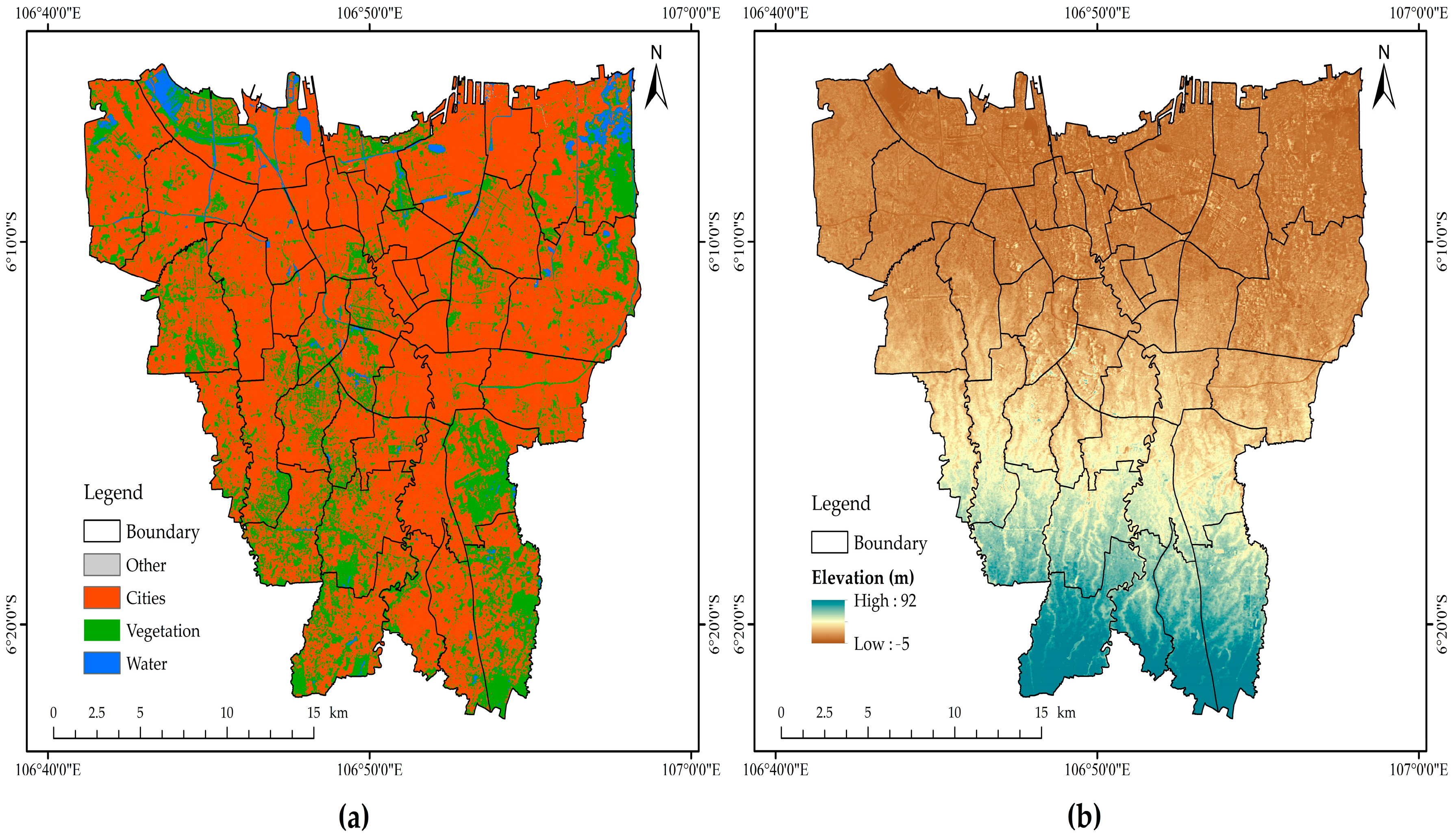
21]. For example, green space counters the deterioration of urban ecological conditions [22], and lower elevation and slope improves road accessibility and rescue-work efficiency [23,24]. The community dimension aims to assess the resistance of communities before the flood disaster and their response capacity afterward. For example, the number of hospitals and shelters can be used to assess a community’s ability to deal with emergency events [17,25]. In addition, the higher the educational level of a community’s residents, the more scientifically and efficiently the community can deal with disaster events [
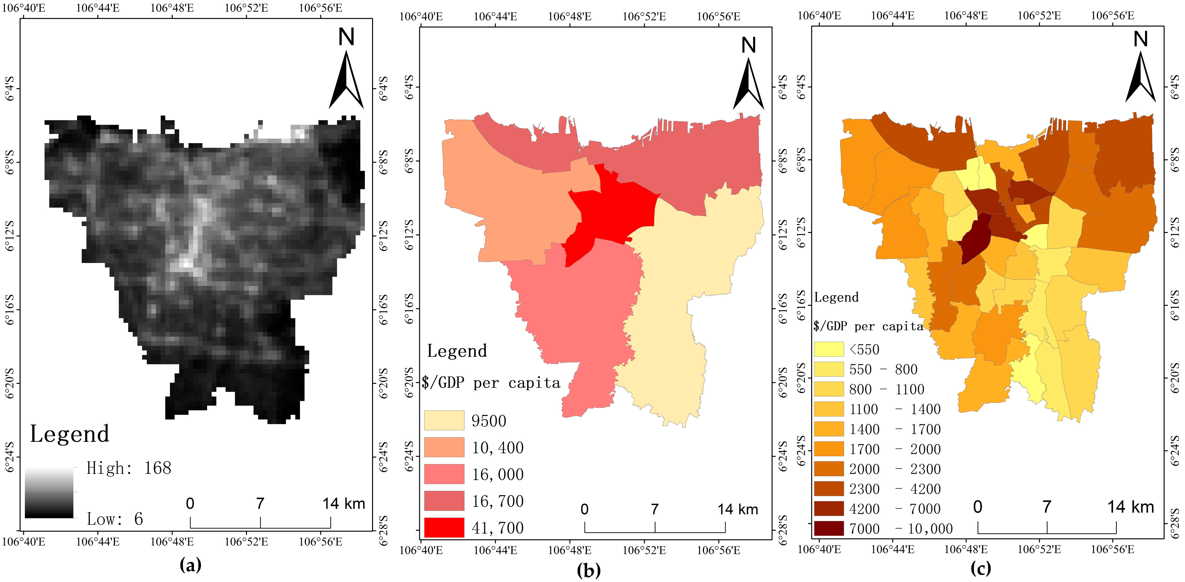
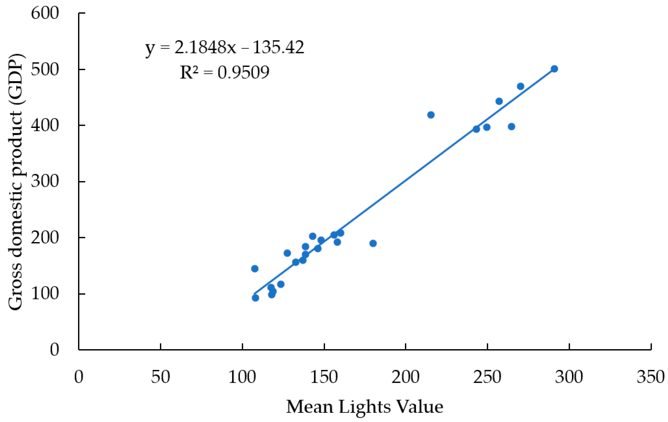
18]. The fourth dimension focuses on economic indicators. Areas with a high GDP per capita and a high POI density will have more financial resources for post-disaster reconstruction after floods than those with lower values of these indicators. Similarly, areas with a high road density have a stronger traffic capacity and more well-developed industries, which means post-disaster rescue operations are easier to perform in these areas than in less road-dense and industry-containing areas [26,27,28]. In addition, space and structure environment are mainly considered in the context of disaster prevention, whereas the dimensions of society and risk management are the focus of post-disaster reconstruction.
The duration and scope of floods, in addition to the losses they cause, must be considered when examining urban resilience to floods [29,30]. Resilience frameworks were previously evaluated through infrastructure-recovery indicators, such as building reconstruction, restoration of public facilities, and productivity recovery [13,31]. Although such infrastructure-recovery indicators are widely used as an indirect reflection of urban resilience [32], the period of flood submergence, namely the time and speed of flood recession, is also a critical aspect of resilience. Few studies have presented a complete urban-resilience evaluation system from the perspective of flood accumulation and release, though the scale and time of floods directly determines the level of infrastructure damage [33,34]. This is mainly due to the difficulty of obtaining relevant data to measure or calculate a continuous flood process, especially in developing countries and poor areas [35]. This poses a challenge to establishing indicators that directly measure flood recovery.
The wide scanning range, low cost, real-time information acquisition, and periodic surface coverage of satellite remote-sensing technology has led to its acceptance as an efficient and appropriate means of extracting and monitoring the changes and areas of floods across various spatiotemporal scales [36,37]. In optical remote-sensing applications, National Oceanic and Atmospheric Administration/Advanced Very High Resolution Radiometer time-series data and Moderate Resolution Imaging Spectroradiometer (MODIS), Landsat, and GaoFen satellite data have been used to dynamically monitor water information [38,39,40]. The continuous and strong absorption of water in the near-infrared and short-wave infrared regions in remote-sensing images has led to the development of different water-detection indexes, such as the normalized differential water index (NDWI) [41], the modified normalized difference water index (MDNWI) [42], the automated water extraction index (AWEI) [6], and the water index (WI) [43]. Although the spatial and temporal resolutions of optical remote-sensing images are constantly improving, their data quality is easily affected by climate conditions, especially clouds [44]. Synthetic aperture radar (SAR) is a remote-sensing microwave sensor that is capable of continuous operation and is sensitive to water [45,46]. European Remote-Sensing Satellite-1 SAR images were used to distinguish flood information based on active contour models comprising grayscale and textural features, and the results showed that this method extracts flood boundaries with high accuracy [47]. Wang, et al. [48] used Sentinel-1A (S1A) data to extract the range of Ebinur Lake, Xinjiang, China, from February 2017 to February 2018 with an accuracy of 99.4%. Moreover, a new water index based on Sentinel-1 data was also used to dynamically monitor changes in water area [49].
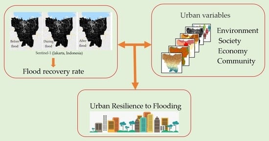
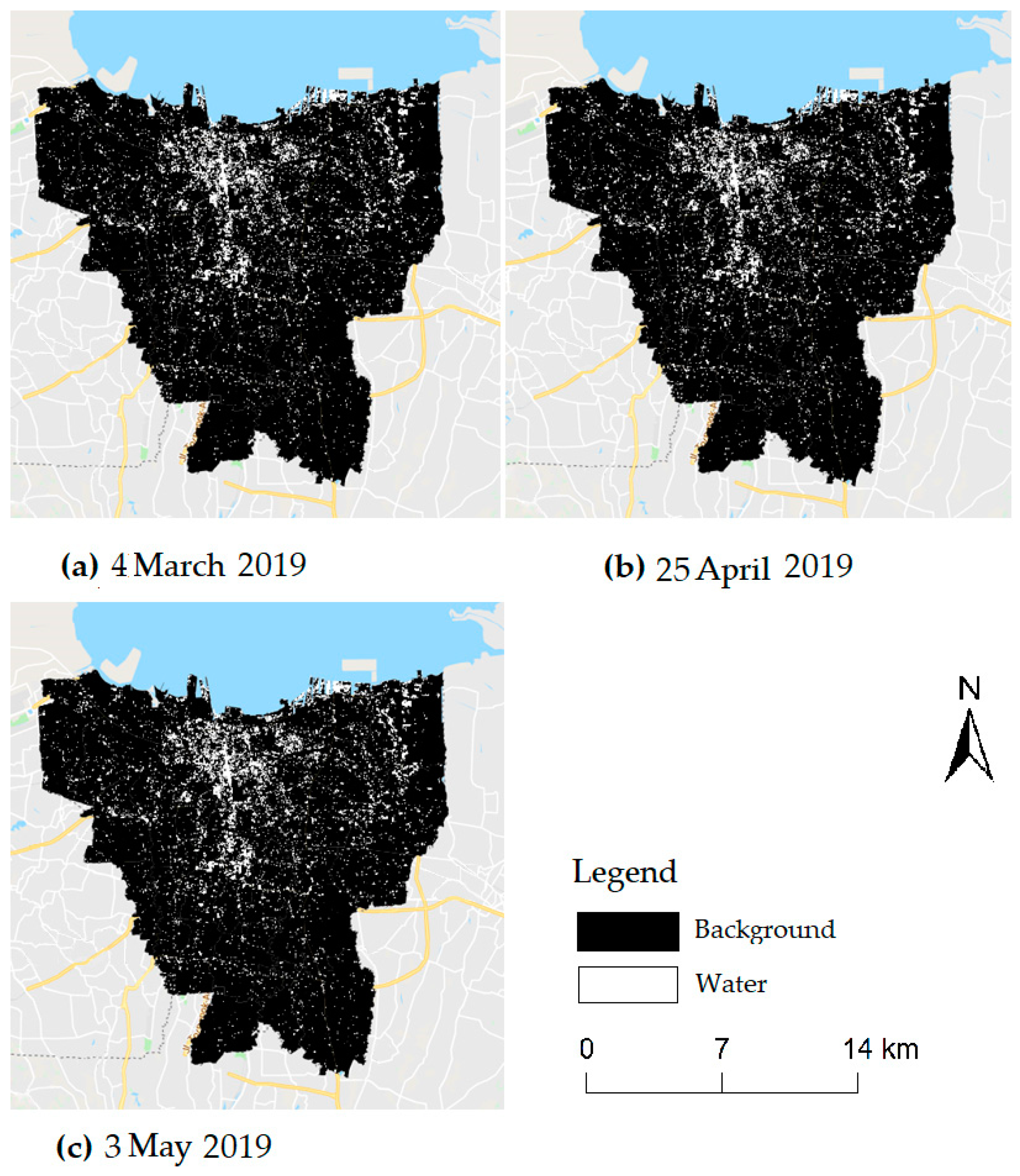
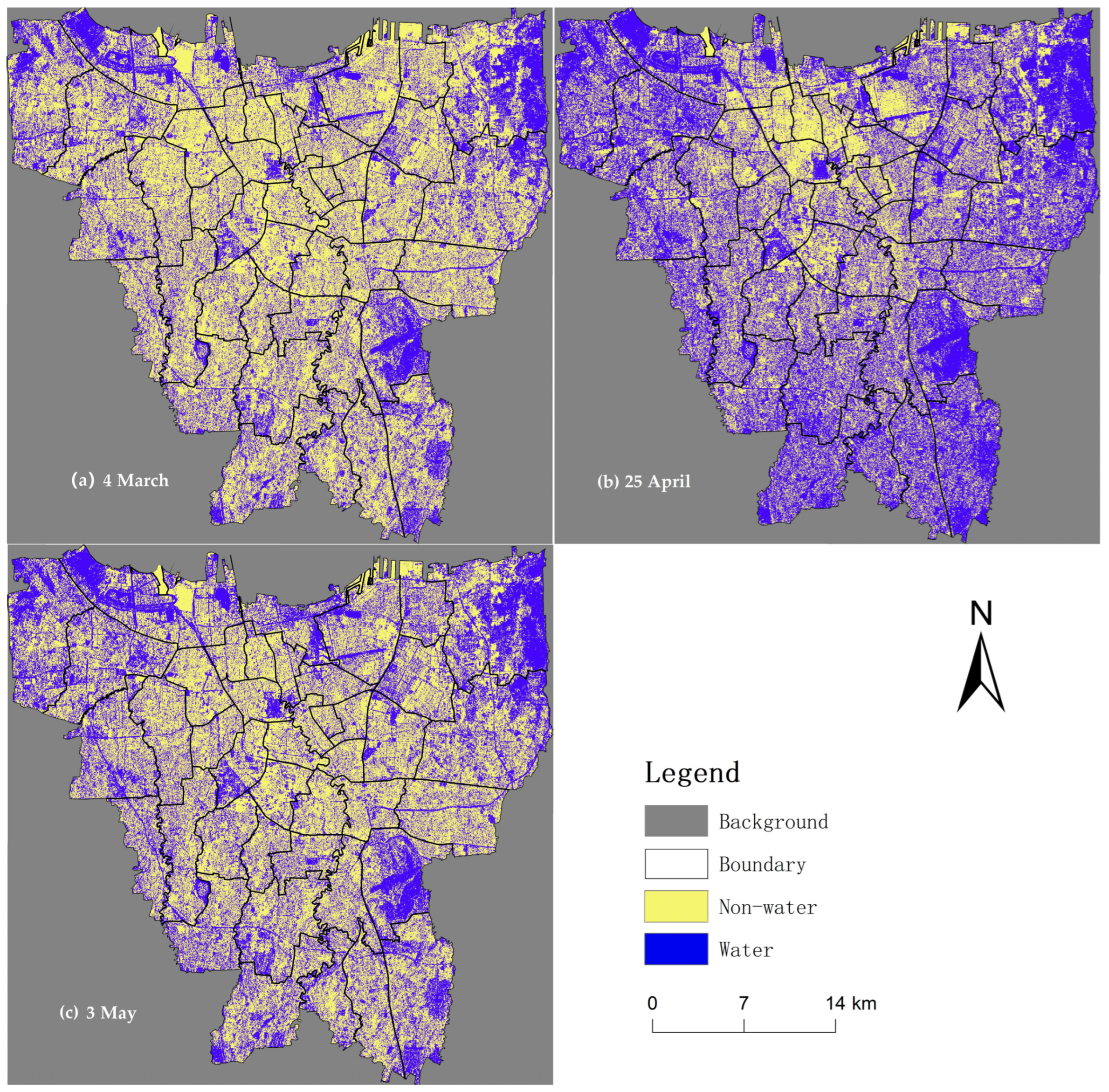
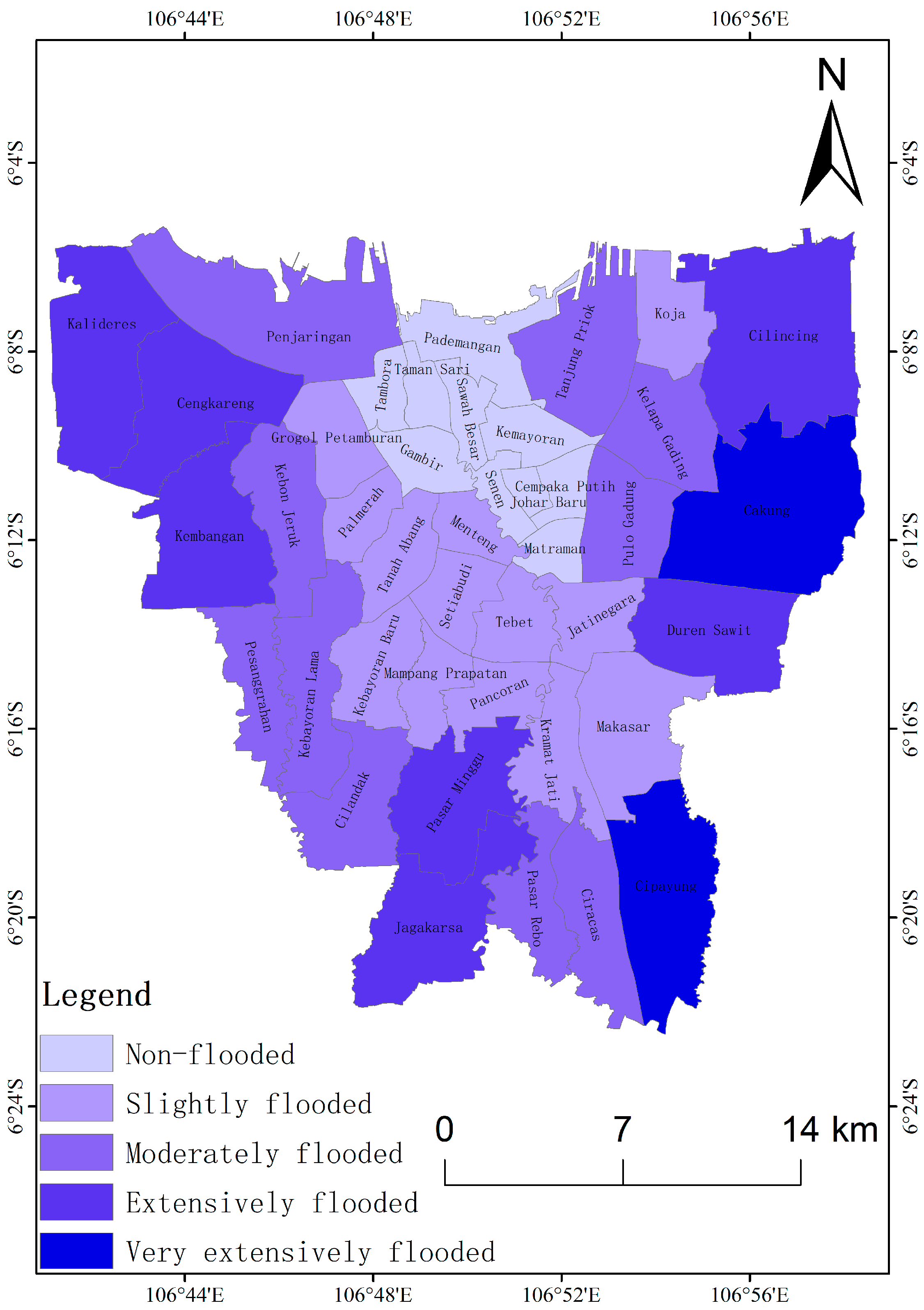
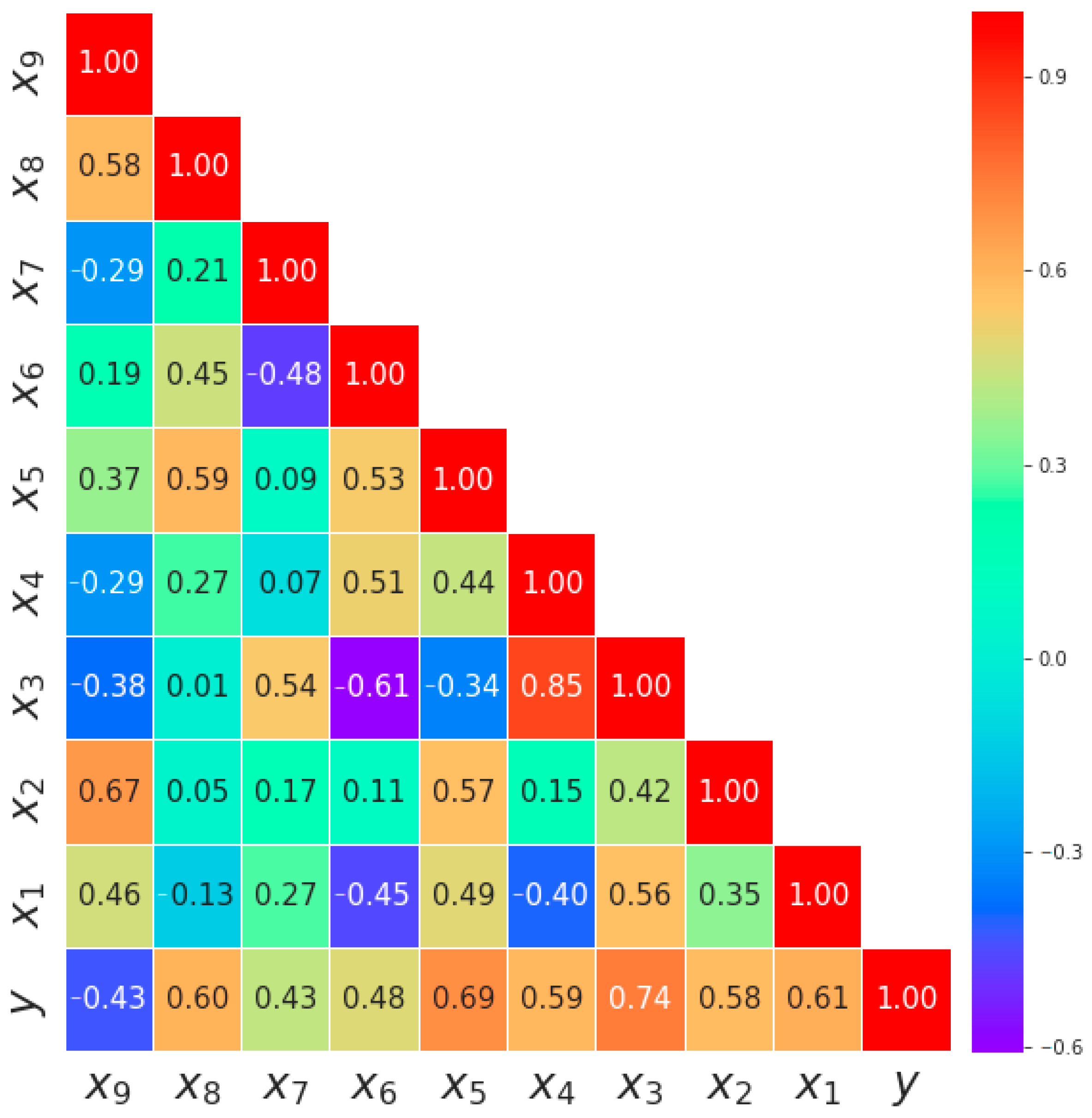
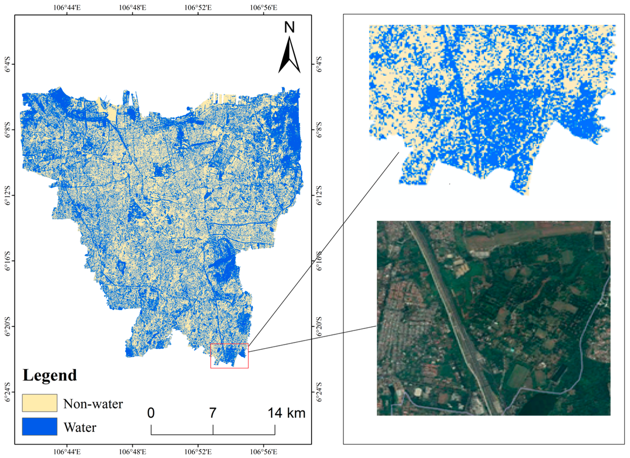
The aim of this study was to examine how to improve the resilience of cities by combining remote-sensing technology with factors from different resilience domains. We attempted to evaluate and analyze urban resilience via a case study of Jakarta, Indonesia, where floods are common in summer. Thus, we used the Otsu model and remote-sensing data to calculate the flood area of 42 different subdistricts in Jakarta on 25 April and 3 May 2019, respectively to compare the speed of flood recession from each of these subdistricts. We also collected the data of factors related to floods in each subdistrict of Jakarta, and used principal component analysis (PCA) to quantify the relative importance of these factors, and their correlations with the speed of flood recession.

2. Materials and Methods

2.1. Study Area

Jakarta is one of the biggest cities in Southeast Asia and also the political, economic, and cultural center of Indonesia. Its urban area is approximately 740 km2, with a population of more than 10 million. Jakarta is composed of six regions, namely East Jakarta, West Jakarta, South Jakarta, North Jakarta, Central Jakarta, and the Thousand Islands. Because the last region has very few people and buildings, it was not included in this study (Figure 1).
In recent years, the increasing unplanned development of the city has caused many urban problems. For example, the vegetative coverage across Jakarta has become very low because of excessive urbanization (Figure 2a) [50]. In addition, as Jakarta is heavily polluted and freshwater resources are scarce, residents overexploit underground water without the government’s permission, thereby causing the surface of Jakarta to sink every year [51,52,53,54]. Consequently, secondary disasters caused by land subsidence frequently occur during urban floods. Moreover, Jakarta is considered one of the most susceptible cities to floods worldwide due to its low elevation and land subsidence, and the heavy rain that it experiences. The average elevation of Jakarta is only 7 m (Figure 2b) according to the Digital Elevation Model (DEM) of this city, and 40% of its area is below sea level [55,56,57]. Some studies and projects of evaluating flood risk have been conducted in Jakarta. For example, the World Bank in partnership with the government of Daerah Khusus Ibukota (DKI) Jakarta conducted a case study in 2011 regarding urban challenges in a changing climate, and the results showed that the greatest climate and disaster-related risk facing Jakarta would be flooding, which may impose very high human and economic costs on the city [2]. Another study investigated the role of social media (Twitter) for civic co-management during monsoon flooding in Jakarta [1]. In addition, a subsequent study utilized Twitter data to assess the effect of residents’ flood evacuation shelters in Jakarta [3]. Nevertheless, assessing urban resilience to flooding in Jakarta using multi-source data that include SAR satellite images is still lacking.
Table 1 shows the three most extensive floods that have occurred in Jakarta in the past two decades, which caused substantial property damage and many casualties. In addition, Jakarta is close to the equator, and has an average annual temperature of 32 °C. Consequently, it has a tropical rainforest climate with rainy and dry seasons, with at least 6 months of rain each year. Finally, Jakarta is adjacent to the Java Sea, and 13 rivers traverse the city, which is another factor that makes it vulnerable to floods.

2.2. Data and Methodology

2.2.1. Remote Sensing Imagery

Sentinel-1 is the first satellite series developed by the European Space Agency for environmental and safety monitoring. The satellite Sentinel-1A (S1A) was launched in April 2014, and some of its parameters are shown in Table 2.
S1A data, a C-band with an Interferometric Wide Swath-Ground Range Detected model (IW-GRD), and VV polarization were obtained from the Google Earth Engine (GEE) platform. GEE is an excellent geographic big-data cloud-computing platform comprising a large database of common satellite data, such as data from Landsat, MODIS, and S1 [60]. These satellite data are available pre-processed and free of charge (Table 3). For example, GEE subjects S1A data to thermal-noise elimination, radiation calibration, topographic correction, and then logarithmic-scaling (10 × log10 (x)) conversion to decibel.
There was no rainfall in Jakarta for 10 days before and after 4 March 2019. Jakarta experienced heavy rain and floods on 25 April, and the weather was clear again on 3 May. Therefore, S1A images of Jakarta on 4 March, 25 April, and 3 May 2019 were selected for this study (Figure 3), as they corresponded to time-points before, during, and after the flood.

2.2.2. Urban Fundamental Datasets

We collected many basic urban variables to represent factors to evaluate resilience, and divided the variables into the four dimensions of society, environment, community, and economy. Table 4 lists all of the variables selected for the experiment. Because the units of measurement for the basic data are not uniform, it is essential to standardize each set of experimental data. The data used in this study are shown in Table 3.
The Indonesian government publishes GDP data for five districts of Jakarta (East Jakarta, West Jakarta, Central Jakarta, South Jakarta, and North Jakarta), but not for their 42 subdistricts. Therefore, we estimated the GDP data of subdistricts by combining the nighttime-light data with the GDP data of the five districts (Figure 4). There is a strong correlation between the nighttime-light data and regional GDP [61,62], and the National Polar-orbiting Partnership Visible Infrared Imaging Radiometer Suite (NPP/VIIRS) is more suitable than the Defense Meteorological Program Operational Line-Scan System at the city scale [63]. Thus, NPP/VIIRS nighttime-light data were used to estimate the GDPs of the 42 subdistricts.
We built a linear regression model based on the nighttime-light data and GDP data of the five districts from 2015 to 2019 (Figure 5). The R2 of the model was 0.95, indicating that most of the observed variation could be explained by the model. All of the parameters were significant at the 95% level. We applied the model to the 42 subdistricts (Table 5), and then collated the predicted GDP values of the subdistricts of every district (Figure 6). A comparison with the actual values showed that the mean absolute percentage error was less than 6.7%, suggesting the high accuracy of estimation using the nighttime light satellite.

2.2.3. Threshold Calculation

The area of flooding is a key evaluation factor for the assessment of urban resilience. Because SAR has a longer wavelength than optical images, this technology can penetrate thick clouds, such as those that exist during continuously rainy conditions, to obtain surface water information, thereby achieving real-time monitoring of the area of flooding. Moreover, SAR is highly sensitive to water bodies; due to the microwave-scattering principle, the pixel value of an SAR image is determined by the echo intensity of every pixel. The reflection of water mainly comprises specular reflection, as water surfaces are smoother than non-water surfaces. Therefore, the backscatter coefficient of water is less than that of land or vegetation, and it appears as a dark tone in the image. At present, water extraction using SAR images is based on textural information, terrain features, independent component analysis, and threshold segmentation. The Otsu model used in this study is a threshold-segmentation method and is one of the most efficient and widely used models [64,65]. The mathematical principle of the Otsu algorithm is described below.
First, the proportions of background and target pixels are calculated by Equations (1) and (2), as follows:
ω 1 = N 1 sum
ω 2 = 1     ω 1 = N 2 sum
where N 1 is the total number of background pixels, ω 1 is the percentage of the sum of the background pixels, N 2 is the total number of target pixels, ω 2 is the percentage of the target pixels, and   sum is the total number of pixels.
Then, the average gray value of pixels in water and non-water areas can be calculated using Equations (3) and (4), respectively:
μ 1 = i = 0 t i   × r ( i | C 0 ) = i = 0 t i   ×   Pi i = 0 t Pi = μ ( t ) ω 1
μ 2 = i = t + 1 M 1 i   ×   Pr ( i | C 1 ) = i = t + 1 M 1 i   ×   Pi i = t + 1 M 1 Pi = μ     μ ( t ) ω 2
where μ1 is the average grayscale of the background, μ2 is the average grayscale of the target, t represents the threshold, M is the maximum gray value of the image, C 0 represents water, and C 1 is non-water.
At last, assuming that the gray value range of the image is [0, 1, 2, …, M], the cumulative gray value from 0 to M is as given by Equation (5), follows:
μ = μ 1   ×   ω 1 + μ 2   ×   ω 2
The between-class variance is calculated by Equation (6), as follows:
g = ω 1   ×   ( μ     μ 1 ) 2   + ω 2   ×   ( μ     μ 2 ) 2
C 0 is [0, 1, …, t] and C1 is [t + 1, t + 2, …, M]. When t is calculated from 0 to M, the entire process iterates a total of M times. The between-class variance g is the optimal segmentation threshold when the value of t corresponds to the maximum.
Therefore, if DN < t in the image (where DN is the value of the backscatter coefficient of the S1A image), the pixel is identified as water; otherwise, the pixel is identified as non-water.

2.2.4. Recovery Rate and Factors’ Weighting

We found that the scattering signal of some smooth roads, roofs, and houses at specific angles would be misinterpreted as water when water was extracted using the backscatter signal of surface targets, and thus the area of water would be overestimated. Therefore, the water area before flooding was subtracted from that during flooding and that after flooding. Mathematical operations were performed on each pixel such that the error generated by the scattering signal of non-water objects at a given location could be minimized.
Based on the same time interval, the mathematical expression of flood recovery rate per unit area is defined as the following formula:
V = S post     S pre S ing     S pre
where S pre , S ing , and S post are the area covered by water before, during, and after flooding in Jakarta, respectively, and V represents the flood recovery rate.
Correlation analysis was performed between each factor and the recovery rate. The original factors were reduced to three independent principal component variables using PCA, and then Equation (8) was used to calculate the coefficients ( C j ) of each factor in the linear combination of different principal components.
C j = F ij CT i
where F ij is the coefficient of the factor in each principal component (where i is the number of principal components and j is the number of factors) and CT i is the characteristic root of the corresponding principal component.
The final step was to assign a weight coefficient to each factor. The weight coefficient differs from the characteristic root coefficient calculated in Equation (8), as it is a quantitative reflection of the positive or negative effect of each factor on the result, whereas the characteristic root coefficient only represents the proportion of each factor in every principal component. In some studies, linear regression was used to construct mathematical expressions of the relationships between factors and dependent variables. The linear regression method has also been widely used to calculate the weight coefficients of factors [27]. This is considered appropriate when factors are independent of each other and the covariance of any two observation residuals is zero. Given the multicollinearity in the factors, the PCA approach was used in this study to reduce the dimension of the factors, and three new independent variables were obtained. The weight coefficients of each factor in the results were deduced from the component matrix and characteristic root by Equation (9), as follows:
W x i = C 1 x i   ×   Var 1 + C 2 x i   ×   Var 2 + C 3 x i   ×   Var 3 Var 1 + Var 2 + Var 3
where C 1 x i , C 2 x i , and C 3 x i represent the coefficients of x i in the first, second, and third principal components, respectively. Var 1 , Var 2 , Var 3 are the characteristic roots of the first, second, and third principal components, respectively.
A schematic diagram of the proposed methodology is shown in Figure 7.

3. Results

3.1. Water Body Extraction

Based on the abovementioned Otsu algorithm, S1A data were used to extract the relevant water body information before (4 March), during (25 April), and after (3 May) a flood in Jakarta (Figure 8). There was no rainfall on 4 March nor on the previous 10 days, but the results suggested that there were water bodies in some areas northwest, northeast, and west of Jakarta because there are some large lakes and rivers in those areas, as shown by Google Earth. The heavy rain on 25 April caused a backflow of seawater and caused lakes and rivers to overflow. Figure 9 shows that most of the city, except for the central region, was flooded by this event. One week later, the floods in most areas had receded, but some residual flooding remained on 3 May.
The severity of the floods in these 42 subdistricts was divided into five levels based on the flooded area (Table 6), namely non-flooded, slightly flooded, moderately flooded, extensively flooded, and very extensively flooded. East Jakarta and West Jakarta suffered the most damage, as shown in Figure 9, which was consistent with the results of local official media reports.
In the same time interval, the flooded area before and after the flood in each subdistrict was calculated. The residual flood area in each subdistrict was calculated accordingly, and the results were then classified according to the statistical methods in Table 7. The central part of Jakarta (e.g., the Pademangan, Taman Sari, Matraman, and Senen regions) and parts of western Jakarta (e.g., the Tebet, Jatinegara, and Kramat Jati regions) had the smallest area of residual flooding, as shown in Figure 10. The areas near the sea in the north (e.g., the Kalideres, Penjaringan, and Cengkareng regions) and near the sea in the west (e.g., the Koja, Cilincing, and Cakung regions) had the largest residual flooded areas.

3.2. Correlation Analysis

In addition to the recovery rate, urban basic conditions are key factors for measuring urban resilience. They have a direct effect on the recovery rate from floods, and different factors in the data have different influences on this effect. For example, the elevation of Jakarta (as represented by a DEM) has a greater effect on the recovery rate than does road density, and the population density has a negative impact on the recovery rate, while the number of hospitals and shelters shows no effect on the same. Therefore, it is necessary to analyze the correlation between the recovery rate and urban basic condition, and then remove factors that are irrelevant to the results. The correlation analysis results (α = 0.05) for the whole area are shown in Figure 11.
The calculation of the correlations between the recovery rate and twelve factors from the four dimensions of society, environment, community, and economy showed that nine factors were strongly correlated with the dependent variable (recovery rate), and the remaining three factors (sex ratio, number of hospitals, and number of shelters) were not correlated with recovery rate. Therefore, the latter three factors were removed in the subsequent calculation, and the remaining nine factors were included in the statistical analysis.

3.3. Coefficient of Each Factor

To quantify the effects of these factors on the results, PCA was used to calculate the coefficient of each factor, where the larger the magnitude of the coefficient, the more important the factor and the greater its effect on the result. First, the Kaiser–Meyer–Olkin (KMO) and Bartlett tests for the nine factors were calculated, as shown in Table 8. The loading matrix is provided in Figure 12. It is generally believed that a KMO measure greater than 0.7 indicates that the selected factor is suitable for PCA. A small p-value (Sig. = 0.000) indicates that the correlation coefficient matrix of the factor is significantly different from the identity matrix, thereby confirming that the original variable is suitable for PCA.
The characteristic roots of the first three principal components and their corresponding contributions and cumulative contributions are shown in Table 9. The characteristic roots of the first, second, and third principal components were all greater than 1, and the cumulative contribution rate was 87.25%, which reflected most of the information of the original nine factors. Therefore, these three principal components were used to replace the original factors. We then calculated the coefficients of each factor in each linear combination of principal components (Figure 13). This process is essential for calculating factor coefficients via PCA.
Finally, the coefficient of each factor was calculated, as shown in Table 10. The order of coefficients was DEM > road density > slope > green area > religion > POI density > GDP > degree of education > population density.

4. Discussion

4.1. Influence of Microwave Remote Sensing Images on the Accuracy of Extraction of Flood Data

In the detection of the flood disaster that occurred in April 2019, an S1A SAR image was used to calculate the backscattering-coefficient characteristics of remote-sensing images of each subdistrict of Jakarta, to determine the segmentation threshold of the extracted flooded and non-flooded areas. Combined with DEM and land cover data, the results showed that the SAR image data were greatly affected by terrain slope and vegetation. Taking the binary image extracted on 4 March as an example (Figure 8a) and comparing it with Google Earth data, it was found that the proportion of blue raster images with a value of 1 in the south of Jakarta is higher than that in the north. This might have occurred because in areas with higher slopes, the surface morphology not only changes the surface microwave radiation characteristics, but also redistributes the hydrothermal energy on the surface. Thus, surface morphology is a key factor in the spatial heterogeneity of areas with higher slopes. The surface radiation-capacity deviation caused by topography is approximately 15 K [66]. Moreover, the terrain is shaded each other, thereby forming a radar shadow on the image, which is misinterpreted as a water body.
Vegetation appeared uneven and black in the microwave remote-sensing images, and was interpreted by the threshold segmentation algorithm as water bodies, as shown in Figure 14. This occurred because microwave radiation is reflected multiple times in the vegetation canopy, thereby causing microwave signals to propagate in different directions. However, most of the resulting signals are not received by the sensor. The vegetation index obtained using microwave remote-sensing data is somewhat correlated with the normalized difference vegetation index calculated from optical remote-sensing data [67,68]. Thus, slope and vegetation will result in a flooded area being calculated as larger than it actually is. Therefore, we performed a displacement calculation to determine the flood area, i.e., the area obtained during the flood minus that before the flood, to minimize the error due to terrain and vegetation.

4.2. Indicator Selection for Different Cases

It is difficult to find one indicator or a set of indicators that can be used as a standard to measure urban resilience, because urban planning, geographical location, and climate all have a major influence on urban resilience. The development of a resilience framework can be based on indicators that require evaluation, rather than available indicators [69]. Indicators of different dimensions must be used for different cities and disasters. There is no consensus on the indicators that affect resilience, which is a challenge for the development of the theoretical framework of resilience. It was found in this study that DEM and slope data had the greatest effect on flood recovery among all of the relevant factors, due to the large difference in elevation between various regions of Jakarta and its very low average elevation. Moreover, the high degree of religious diversity in Jakarta was found to play a significant role in flood recovery. Generally, people of the same religion were more united than those of different religions, and thereby the former dealt with emergencies with greater efficiency than the latter. However, we found that the flood recovery rate decreased as the population density increased. This is due to the fact that the living areas of the rich in Jakarta are of low population density, whereas those of the poor are of high population density. Thus, floods cannot be dealt with in a timely manner in the very crowded and deficient areas of the poor.

4.3. Strategies for Improving Urban Flood Resilience

Priority can be given to factors related to urban resilience in future urban planning, and corresponding policies and measures should then be formulated. Specifically, environmental indicators are recommended as the first option to improve urban resilience in Jakarta, such as strictly controlling groundwater extraction that causes surface subsidence. Economic indicators are also very important for urban construction and development; the government must provide more rescue resources and policy support to regions with poor infrastructure for construction and economic development. Traffic conditions in underdeveloped road-network areas must also be improved, such that relief can be provided more rapidly.
Floods are the most common natural disaster and pose a great threat to most cities prone to waterlogging. Thus, making a scientific and rational flood control and disaster reduction plans is urgently needed. Based on the selected indicators and the evaluation results of resilience to floods, the following suggestions for improving the flood resilience are provided. First, the driving force of urban development and residents’ well-being depend largely on local economy, and urban flooding prevention and mitigation facilities and post-flooding reconstruction efforts are also inseparable from the city’s financial support. Therefore, improving the level of local economy is a key step to improve the city’s flood resilience. Second, infrastructure is crucial for the normal operation of the city. In particular, infrastructure plays a significant role in pre-disaster resistance and post-disaster recovery. Finally, eco-city is a main direction of sustainable and green development of cities. With the continuous expansion of urban areas and the increasing urban population, the contradiction between ecological conservation and development has become apparent. Greenland, lake areas and river courses should be restored to enhance water absorption and water-fixing capacities during heavy rains and floods.

5. Conclusions

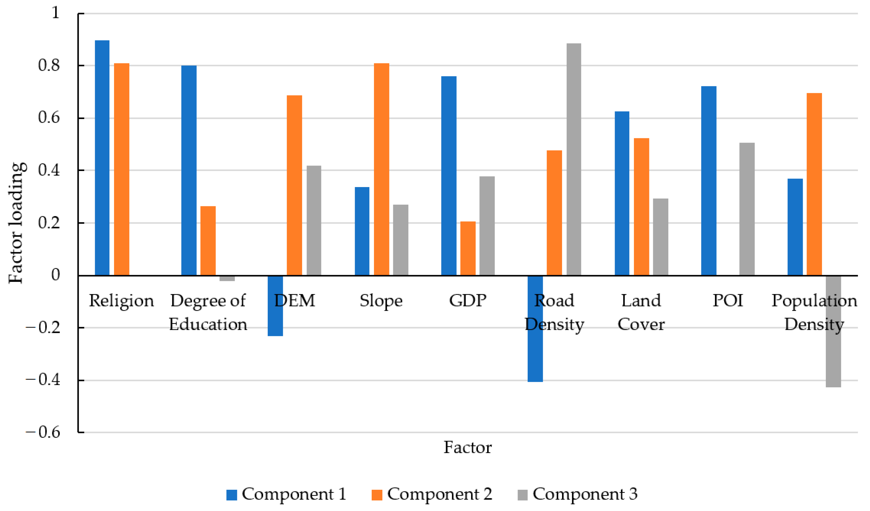
This study used remote-sensing data combined with multiple dimensions of urban factors to calculate and analyze the differences and causes of urban resilience in different regions. The S1A data on three dates were used to extract the flooded area, and the changes in these areas, using the Otsu method. In addition, urban basic data such as the POI, GDP, and DEM were used to analyze the correlation between the flooded area and the recovery rate (Sig. < 0.05). Irrelevant data were then removed and the remaining data were used as factors for urban resilience. Finally, PCA was employed to reduce the dimensionality of high-dimensional factors, and the original nine factors were replaced by three principal components (total explanation > 90%). The weight coefficient of each factor was calculated by the characteristic root, variance contribution of the principal components, and the loading matrix of the original factor.
Remote sensing overcomes the problem of obtaining large-scale flood boundaries, especially for areas without meteorological and hydrological stations, which improves the accuracy of flood-flow calculations and provides a more accurate basis for disaster reduction and preventing floods. In addition, the data we used in this study can be provided to support flooding projects, such as sponge city, water-sensitive urban design, low-impact development. Moreover, this method provides a new direction for the selection of indicators for the evaluation of resilience frameworks, and to guide urban responses to natural disasters.
The limitations of experimental conditions indicate that there is still room for improvement of study. For example, new indicators could be added to improve the correlations between various factors and flood-recovery rates, such as climate factors that are directly related to the occurrence of floods (real-time precipitation, precipitation time, etc.) and factors related to community-street flood drainage (length of urban underground water pipes, number of sewer covers, length of the dike, urban communication coverage, etc.). Furthermore, this study mainly measured regional resilience from the perspective of urban post-disaster recovery, but urban vulnerability and property loss (i.e., the number of buildings damaged and number of casualties) may also be used as dimensions to measure urban resilience. Subsequent studies will attempt to add these data (if available) to the urban infrastructure database, and examine their contributions to urban resilience.

Author Contributions

Conceptualization: B.H., X.L., Q.G. and Y.H.; methodology: B.H., X.L. and Q.G.; spatial data analysis: H.Z., X.L., Q.G. and R.L.; Original draft writing: X.L. and H.Z.; Review and editing: Y.X., Y.Q., R.L., B.H. and Y.H. All authors have read and agreed to the published version of the manuscript.

Funding

This research was supported by United Nations Economic and Social Commission for Asia and the Pacific (10141267), the Hong Kong Research Grants Council (AoE/E-603/18), and the National Key R&D Program of China (2019YFC1510400).

Institutional Review Board Statement

Not applicable.

Informed Consent Statement

Not applicable.

Data Availability Statement

Satellite Sentinel-1A images are freely available from Google Earth Engine (GEE); road density, the number of hospitals and shelters data from Badan Penanggulangan Bencana Daerah (https://bpbd.jakarta.go.id/profile accessed on 8 April 2022); Digital Elevation Models (DEMs) from Seamless Digital Elevation Model (DEM) dan Batimetri Nasional (https://tanahair.indonesia.go.id/demnas/#/ accessed on 8 April 2022); land-cover maps from the open source data website of Tsinghua University of China (http://data.ess.tsinghua.edu.cn/?%20tdsourcetag=s_pcqq_aiomsg accessed on 8 April 2022); population density, sex ratio, and religion data from Badan Pusat Statistik (http://www.bps.go.id accessed on 8 April 2022); gross domestic product (GDP) data from Badan Penanggulangan Bencana Daerah (https://bpbd.jakarta.go.id/profile accessed on 8 April 2022); points-of-interest (POIs) from Baidu Map Services (http://lbsyun.baidu.com/ accessed on 8 April 2022); and National Polar-orbiting Partnership Visible Infrared Imaging Radiometer Suite (NPP/VIIRS) nighttime-light images from the National Oceanic and Atmospheric Administration (https://www.ngdc.noaa.gov/eog/viirs accessed on 8 April 2022).

Acknowledgments

We would like to thank Baidu Maps, Badan Penanggulangan Bencana Daerah Provinsi DKI Jakarta, Google Earth Engine, Tsinghua University, the National Oceanic and Atmospheric Administration, and OpenStreetMap for providing us with the data used in this study.

Conflicts of Interest

The authors declare no conflict of interest.

References

  1. Tomas, H.; Etienne, T. White Paper-PetaJakarta.org: Assessing the Role of Social Media for Civic Co-Management During Monsoon Flooding in Jakarta, Indonesia; University of Wollongong: Wollongong, Peta Jakarta, 2015; Available online: https://petajakarta.org/banjir/en/research/index.html (accessed on 8 April 2022).
  2. The World Bank. JAKARTA|Urban Challenges in a Changing Climate. Mayors’ Task Force on Climate Change, Disaster Risk & the Urban Poor. 2011. Available online: https://documents1.worldbank.org/curated/en/132781468039870805/pdf/650180WP0Box360ange0Jakarta0English.pdf (accessed on 8 April 2022).
  3. Kusumo, A.N.L.; Reckien, D.; Verplanke, J. Utilising volunteered geographic information to assess resident’s flood evacuation shelters. Case Study Jkt. Appl. Geogr. 2017, 88, 174–185. [Google Scholar] [CrossRef]
  4. Nan, S. Introduction to habitat III and new city agenda, and their inspiration to China. City Plan. Rev. 2017, 41, 9–21. [Google Scholar]
  5. Moghadas, M.; Asadzadeh, A.; Vafeidis, A.; Fekete, A.; Kötter, T. A multi-criteria approach for assessing urban flood resilience in Tehran, Iran. Int. J. Disaster Risk Reduct. 2019, 35, 101069. [Google Scholar] [CrossRef]
  6. Feyisa, G.L.; Meilby, H.; Fensholt, R.; Proud, S.R. Automated Water Extraction Index: A new technique for surface water mapping using Landsat imagery. Remote Sens. Environ. 2014, 140, 23–35. [Google Scholar] [CrossRef]
  7. Zhang, X.; Song, J.; Peng, J.; Wu, J. Landslides-oriented urban disaster resilience assessment—A case study in ShenZhen, China. Sci. Total Environ. 2019, 661, 95–106. [Google Scholar] [CrossRef]
  8. Song, J.; Huang, B.; Li, R. Measuring Recovery to Build up Metrics of Flood Resilience Based on Pollutant Discharge Data: A Case Study in East China. Water 2017, 9, 619. [Google Scholar] [CrossRef]
  9. Ya, L.; Zhai, G. China’s Urban Disaster Resilience Evaluation and Promotion. Planners 2017, 33, 5–11. [Google Scholar]
  10. Vamvakeridou-Lyroudia, L.; Chen, A.; Khoury, M.; Gibson, M.; Kostaridis, A.; Stewart, D.; Wood, M.; Djordjevic, S.; Savic, D. Assessing and visualising hazard impacts to enhance the resilience of Critical Infrastructures to urban flooding. Sci. Total Environ. 2020, 707, 136078. [Google Scholar] [CrossRef]
  11. He, B.J.; Zhu, J.; Zhao, D.X.; Gou, Z.H.; Qi, J.D.; Wang, J. Co-benefits approach: Opportunities for implementing sponge city and urban heat island mitigation. Land Use Policy 2019, 86, 147–157. [Google Scholar] [CrossRef]
  12. Sayers, P.; Li, Y.; Galloway, G.; Penning-Rowsell, E.; Shen, F.; Wen, K.; Chen, Y.; Le Quesne, T. Flood Risk Management: A Strategic Approach; UNESCO: Paris, France, 2013. [Google Scholar]
  13. Chang, S.E. Urban disaster recovery: A measurement framework and its application to the 1995 Kobe earthquake. Disasters 2010, 34, 303–327. [Google Scholar] [CrossRef]
  14. Jordan, E.; Javernick-Will, A.; Tierney, K. Post-tsunami recovery in Tamil Nadu, India: Combined social and infrastructural outcomes. Nat. Hazards 2016, 84, 1327–1347. [Google Scholar] [CrossRef]
  15. Cutter, S.L. The landscape of disaster resilience indicators in the USA. Nat. Hazards 2016, 80, 1–18. [Google Scholar] [CrossRef]
  16. Olshansky, R.; Johnson, L.; Topping, K. Rebuilding communities following disaster: Lessons from Kobe and Los Angeles. Built Environ. 2006, 32, 354–374. [Google Scholar] [CrossRef]
  17. Cutter, S. A Framework for Measuring Coastal Hazard Resilience in New Jersey Communities; White Paper for the Urban Coast Institute: West Long Branch, NJ, USA, 2008; Available online: https://www.co.monmouth.nj.us/documents/104/CoastalHazardResilientCommunities.pdf (accessed on 15 January 2021).
  18. Cutter, S.L.; Bryan, B.J.; Shirley, W.L. Social Vulnerability to Environmental Hazards. Soc. Sci. Quart. 2003, 84, 242–261. [Google Scholar] [CrossRef]
  19. Song, J.; Huang, B.; Li, R. Assessing local resilience to typhoon disasters: A case study in Nansha, Guangzhou. PLoS ONE 2018, 13, e0190701. [Google Scholar] [CrossRef] [PubMed] [Green Version]
  20. Orencio, P.M.; Fujii, M. A localized disaster-resilience index to assess coastal communities based on an analytic hierarchy process (AHP). Int. J. Disaster Risk Reduct. 2013, 3, 62–75. [Google Scholar] [CrossRef]
  21. Lhomme, S.; Serre, D.; Diab, Y.; Laganier, R. GIS development for urban flood resilience. WIT Trans. Ecol. Environ. 2010, 129, 661–671. [Google Scholar] [CrossRef]
  22. Yoon, D.K.; Kang, J.E.; Brody, S.D. A measurement of community disaster resilience in Korea. J. Environ. Manag. 2016, 59, 436–460. [Google Scholar] [CrossRef]
  23. Haynes, K.E.; Georgianna, T.D. Risk assessment of water allocation and pollution treatment policies in a regional economy: Reliability, vulnerability and resiliency in the Yellowstone Basin of Montana. Comput. Environ. Urban Syst. 1989, 13, 75–94. [Google Scholar] [CrossRef]
  24. Reams, M.A.; Lam, N.S.N.; Baker, A. Measuring Capacity for Resilience among Coastal Counties of the US Northern Gulf of Mexico Region. Am. J. Clim. Chang. 2012, 1, 194–204. [Google Scholar] [CrossRef] [Green Version]
  25. Liao, K.; Kuei, H. A Theory on Urban Resilience to Floods--A Basis for Alternative Planning Practices. Ecol. Soc. 2012, 17, 48. [Google Scholar] [CrossRef]
  26. Li, X.; Lam, N.; Qiang, Y.; Li, K.; Yin, L.; Liu, S.; Zheng, W. Measuring County Resilience After the 2008 Wenchuan Earthquake. Int. J. Disaster Risk Sci. 2016, 7, 393–412. [Google Scholar] [CrossRef] [Green Version]
  27. Wood, N.J.; Burton, C.G.; Cutter, S.L. Community variations in social vulnerability to Cascadia-related tsunamis in the U.S. Pacific Northwest. Nat. Hazards 2010, 52, 369–389. [Google Scholar] [CrossRef] [Green Version]
  28. Cutter, S.L.; Barnes, L.; Berry, M.; Burton, C.; Evans, E.; Tate, E.; Webb, J. A place-based model for understanding community resilience to natural disasters. Glob. Environ. Chang. 2008, 18, 598–606. [Google Scholar] [CrossRef]
  29. Mileti, D. Disasters by Design: A Reassessment of Natural Hazards in the United States; Joseph Henry Press: Washington, DC, USA, 1999. [Google Scholar] [CrossRef]
  30. Phillips, B. Disaster Recovery; CRC Taylor & Francis Press: Boca Raton, FL, USA, 2015. [Google Scholar]
  31. Mieler, M.; Stojadinovic, B.; Budnitz, R.; Comerio, M.; Mahin, S. A Framework for Linking Community-Resilience Goals to Specific Performance Targets for the Built Environment. Earthq. Spectra 2015, 31, 1267–1283. [Google Scholar] [CrossRef] [Green Version]
  32. Burton, C.G. A validation of metrics for community resilience to natural hazards and disasters using the recovery from Hurricane Katrina as a case study. Ann. Assoc. Am. Geogr. 2015, 105, 67–86. [Google Scholar] [CrossRef]
  33. Tierney, K.; Oliver, A. Social dimensions of disaster recovery. Int. J. Mass Emergencies Disasters 2012, 30, 123–146. [Google Scholar]
  34. Olshansky, R. Toward a Theory of Community Recovery from Disaster: A Review of Existing Literature. In Proceedings of the First International Conference of Urban Disaster Reduction, Kobe, Japan, 19 January 2005. [Google Scholar]
  35. Gall, M. From Social Vulnerability to Resilience: Measuring Progress toward Disaster Risk Reduction; United Nations University Institute for Environment and Human Security (UNU-EHS): Bonn, Germany, 2013; Available online: http://www.ehs.unu.edu/file/get/11125.pdf (accessed on 15 January 2021). [CrossRef]
  36. Feng, L.; Hu, C.; Chen, X.; Li, R.; Murch, B. MODIS observations of the bottom topography and its inter-annual variability of Poyang Lake. Remote Sens. Environ. 2012, 115, 2729–2741. [Google Scholar] [CrossRef]
  37. Haas, E.M.; Bartholomé, E.; Lambin, E.F.; Vanacker, V. Remotely sensed surface water extent as an indicator of short-term changes in ecohydrological processes in sub-Saharan Western Africa. Remote Sens. Environ. 2011, 115, 3436–3445. [Google Scholar] [CrossRef]
  38. Sheng, Y.; Gong, P.; Xiao, Q. Quantitative dynamic flood monitoring with NOAA AVHRR. Int. J. Remote Sens. 2010, 22, 1709–1724. [Google Scholar] [CrossRef]
  39. Lian, F.; Hu, C.; Chen, X.; Cai, X.; Tian, L.; Gan, W. Assessment of inundation changes of Poyang Lake using MODIS observations between 2000 and 2010. Remote Sens. Environ. 2012, 121, 80–92. [Google Scholar] [CrossRef]
  40. Liao, A.; Chen, L.; Chen, J.; He, C.; Cao, X.; Chen, J.; Peng, S.; Sun, F.; Gong, P. High-resolution remote sensing mapping of global land water. Sci. China Earth Sci. 2014, 57, 2305–2316. [Google Scholar] [CrossRef]
  41. Mcfeeters, S.K. The use of the Normalized Difference Water Index (NDWI) in the delineation of open water features. Int. J. Remote Sens. 1996, 17, 1425–1432. [Google Scholar] [CrossRef]
  42. Xu, H. Modification of normalised difference water index (NDWI) to enhance open water features in remotely sensed imagery. Int. J. Remote Sens. 2007, 27, 3025–3033. [Google Scholar] [CrossRef]
  43. Ji, L.; Peng, G.; Geng, X.; Zhao, Y. Improving the Accuracy of the Water Surface Cover Type in the 30 m FROM-GLC Product. Remote Sens. 2015, 7, 13507–13527. [Google Scholar] [CrossRef] [Green Version]
  44. Ulaby, F.T.; Elachi, C. Radar polarimetry for geoscience applications. Geocarto Int. 1990, 5, 38. [Google Scholar] [CrossRef]
  45. Mason, D.; Schumann, G.P.; Neal, J.; Garcia-Pintado, J.; Bates, P. Automatic near real-time selection of flood water levels from high resolution Synthetic Aperture Radar images for assimilation into hydraulic models: A case study. Remote Sens. Environ. 2012, 124, 705–716. [Google Scholar] [CrossRef] [Green Version]
  46. Jin, H.; Mountrakis, G.; Stehman, S.V. Assessing integration of intensity, polarimetric scattering, interferometric coherence and spatial texture metrics in PALSAR-derived land cover classification. ISPRS J. Photogramm. Remote Sens. 2014, 98, 70–84. [Google Scholar] [CrossRef]
  47. Horritt, M.; Mason, D.; Luckman, A. Flood boundary delineation from synthetic aperture radar imagery using a statistical active contour model. Int. J. Remote Sens. 2001, 22, 2489–2507. [Google Scholar] [CrossRef]
  48. Wang, J.; Ding, J.; Li, G.; Liang, J.; Yu, D.; Aishan, T.; Zhang, F.; Yang, J.; Abulimiti, A.; Liu, J. Dynamic detection of water surface area of Ebinur Lake using multi-source satellite data (Landsat and Sentinel-1A) and its responses to changing environment. Catena 2019, 177, 189–201. [Google Scholar] [CrossRef]
  49. Tian, H.; Li, W.; Wu, M.; Huang, N.; Li, G.; Li, X.; Niu, Z. Dynamic monitoring of the largest freshwater lake in China using a new water index derived from high spatiotemporal resolution Sentinel-1A data. Remote Sens. 2017, 9, 521. [Google Scholar] [CrossRef] [Green Version]
  50. Gong, P.; Liu, H.; Zhang, M.; Li, C.; Wang, J.; Huang, H.; Clinton, N.; Ji, L.; Li, W.; Bai, Y.; et al. Stable classification with limited sample: Transferring a 30-m resolution sample set collected in 2015 to mapping 10-m resolution global land cover in 2017. Sci. Bull. 2019, 64, 370–373. [Google Scholar] [CrossRef] [Green Version]
  51. Firman, T. The continuity and change in mega-urbanization in Indonesia: A survey of Jakarta–Bandung Region (JBR) development. Habitat Int. 2009, 33, 327–339. [Google Scholar] [CrossRef]
  52. Varrani, A.; Nones, M. Vulnerability, impacts and assessment of climate change on Jakarta and Venice. Int. J. River Basin Manag. 2017, 16, 439–447. [Google Scholar] [CrossRef]
  53. Bakr, M. Influence of Groundwater Management on Land Subsidence in Deltas. Water Resour. Manag. 2015, 29, 1541–1555. [Google Scholar] [CrossRef]
  54. Goh, K. Urban Waterscapes: The Hydro-Politics of Flooding in a Sinking City. Int. J. Urban Reg. Res. 2019, 43, 250–272. [Google Scholar] [CrossRef]
  55. Mark, C.; Peter, J.M.N.; Paratiwo, M.R. Flooding in Jakarta Towards a blue city with improved water management. J. Humanit. Soc. Sci. Southeast Asia 2009, 161, 454–484. [Google Scholar] [CrossRef]
  56. Budiyono, Y.; Aerts, J.; Brinkman, J.; Marfai, M.A.; Ward, P. Flood risk assessment for delta mega-cities: A case study of Jakarta. Nat. Hazards 2014, 75, 389–413. [Google Scholar] [CrossRef]
  57. Ward, P.J.; Marfai, M.A.; Yulianto, F.; Hizbaron, D.R.; Aerts, J.C.J.H. Coastal inundation and damage exposure estimation: A case study for Jakarta. Nat. Hazards 2010, 56, 899–916. [Google Scholar] [CrossRef] [Green Version]
  58. Sagala, S.; Lassa, J.; Yasaditama, H.; Hudalah, D. The Evolution of Risk and Vulnerability in Greater Jakarta: Contesting Government Policy in Dealing with a Megacity’s Exposure to Flooding; Institute of Resource Governance and Social Change (IRGSC): Kupang, Indonesia, 2013; Available online: https://www.preventionweb.net/publications/view/30611 (accessed on 15 January 2021).
  59. Wijayanti, P.; Zhu, X.; Hellegers, P.; Budiyono, Y.; van Ierland, E.C. Estimation of river flood damages in Jakarta, Indonesia. Nat. Hazards 2017, 86, 1059–1079. [Google Scholar] [CrossRef] [Green Version]
  60. Gorelick, N.; Hancher, M.; Dixon, M.; Ilyushchenko, S.; Thau, D.; Moore, R. Google Earth Engine: Planetary-scale geospatial analysis for everyone. Remote Sens. Environ. 2017, 202, 18–27. [Google Scholar] [CrossRef]
  61. Henderson, J.V.; Storeygard, A.; Weil, D.N. Measuring Economic Growth from Outer Space. Am. Econ. Rev. 2012, 102, 994–1028. [Google Scholar] [CrossRef] [PubMed] [Green Version]
  62. Ma, T.; Zhou, C.; Pei, T.; Haynie, S.; Fan, J. Responses of Suomi-NPP VIIRS-derived nighttime lights to socioeconomic activity in China’s cities. Remote Sens. Lett. 2014, 5, 165–174. [Google Scholar] [CrossRef]
  63. Dai, Z.; Hu, Y.; Zhao, G. The suitability of different nighttime light data for GDP estimation at different spatial scales and regional levels. Sustainability 2017, 9, 305. [Google Scholar] [CrossRef] [Green Version]
  64. Otsu, N. A threshold selection method from gray-level histograms. IEEE Trans. Syst. Man Cybern. 1979, 9, 62–66. [Google Scholar] [CrossRef] [Green Version]
  65. Rosser, J.F.; Leibovici, D.; Jackson, M. Rapid flood inundation mapping using social media, remote sensing and topographic data. Nat. Hazards 2017, 87, 103–120. [Google Scholar] [CrossRef] [Green Version]
  66. Pierdicca, N.; Pulvirenti, L.; Marzano, F.S. Simulating topographic effects on spaceborne radiometric observations between L and X frequency bands. IEEE Trans. Geosci. Remote Sens. 2009, 48, 273–282. [Google Scholar] [CrossRef]
  67. Choudhury, B.; Tucker, C.; Golus, R.; Newcomb, W. Monitoring vegetation using Nimbus-7 scanning multichannel microwave radiometer’s data. Int. J. Remote Sens. 1987, 8, 533–538. [Google Scholar] [CrossRef]
  68. Paloscia, S.; Pampaloni, P. Microwave vegetation indexes for detecting biomass and water conditions of agricultural crops. Remote Sens. Environ. 1992, 40, 15–26. [Google Scholar] [CrossRef]
  69. Commission, J.R.C.E. Handbook on Constructing Composite Indicators: Methodology and User Guide; OECD Publishing: Paris, France, 2008. [Google Scholar]
Figure 1. Study area (Source: Google map).
Remotesensing 14 02010 g001
Figure 2. The land cover (a) and Digital Elevation Model (b) of Jakarta.
Remotesensing 14 02010 g002
Figure 3. Sentinel-1A remote sensing images of Jakarta.
Remotesensing 14 02010 g003
Figure 4. Nighttime-light image (a), gross domestic product (GDP) of five districts (b), and simulated GDP of 42 subdistricts (c).
Remotesensing 14 02010 g004
Figure 5. Regression model of GDP and mean lights value.
Remotesensing 14 02010 g005
Figure 6. Actual gross domestic product (GDP) of the five districts and the sum of the predicted GDP of their subdistricts.
Remotesensing 14 02010 g006
Figure 7. Schematic diagram of the proposed methodology.
Remotesensing 14 02010 g007
Figure 8. Water bodies in Jakarta on 4 March (a), 25 April (b), and 3 May (c).
Remotesensing 14 02010 g008
Figure 9. The severity of flooding in 42 sub-districts of Jakarta.
Remotesensing 14 02010 g009
Figure 10. Flood recovery rate in 42 sub-districts.
Remotesensing 14 02010 g010
Figure 11. Correlations between the recovery rate (y), religion ( x 1 ), education level ( x 2 ), mean digital elevation model ( x 3 ), mean slope ( x 4 ), gross domestic product ( x 5 ), road density ( x 6 ), mean green area ( x 7 ), points-of-interest density ( x 8 ), and population density ( x 9 ).
Remotesensing 14 02010 g011
Figure 12. Factor loading.
Remotesensing 14 02010 g012
Figure 13. Coefficient of each factor in the principal components.
Remotesensing 14 02010 g013
Figure 14. Example of vegetation being misinterpreted as water.
Remotesensing 14 02010 g014
Table 1. Damage caused by three of the worst floods in Jakarta [58,59].
YearInundation Area (km2)Displaced PopulationEconomic Loss (USD)
199626430,000137 million
2007400500,000572 million
201346340,000775 million
Table 2. Sentinel-1A parameters.
ModeResolution (m²)Swath (km)Polarization
Strip Map4 × 580VV + VH or HH + HV
Interferometric-Wide swath5 × 20240VV + VH or HH + HV
Extra-Wide swath25 × 80400VV +VH or HH + HV
Wave mode20 × 520 × 20HH or VV
Note: HH = horizontal transmit, horizontal receive, HV = horizontal transmit, vertical receive, VH = vertical transmit, horizontal receive, and VV = vertical transmit, vertical receive.
Table 3. Data used in this study.
DataSourceYear
Satellite Sentinel-1A (S1A) Google Earth Engine (GEE)4 March, 25 April, and 3 May 2019
Road density and number of hospitals and shelters (subdistricts)Badan Penanggulangan Bencana Daerah (https://bpbd.jakarta.go.id/profile accessed on 15 June 2021)2018
Digital Elevation Model (DEM) (8 m) and slope calculated by DEMSeamless Digital Elevation Model (DEM) dan Batimetri Nasional (https://tanahair.indonesia.go.id/demnas/#/ accessed on 10 April 2022) 2016
Land-cover data (10 m)the open source data website of Tsinghua University of China (http://data.ess.tsinghua.edu.cn/?%20tdsourcetag=s_pcqq_aiomsg accessed on 10 April 2022)2017
Population density, sex ratio, and religion data (subdistricts)Badan Pusat Statistik (http://www.bps.go.id accessed on 15 June 2021)2015
Gross domestic product (GDP) data (districts)Badan Penanggulangan Bencana Daerah (https://bpbd.jakarta.go.id/profile accessed on 15 June 2021)2015, 2016, 2017, 2018, 2019
Points-of-interest (POI) dataBaidu Map Services (http://lbsyun.baidu.com/ accessed on 15 June 2021)2019
National Polar-orbiting Partnership Visible Infrared Imaging Radiometer Suite (NPP/VIIRS) nighttime-light data (500 m)the National Oceanic and Atmospheric Administration (https://www.ngdc.noaa.gov/eog/viirs accessed on 15 June 2021)2015, 2016, 2017, 2018, 2019
Table 4. Variables representing the four dimensions of urban resilience.
DimensionLabelMeasure
Community DimensionNumber of hospitalsNumber of hospitals per subdistrict
Number of sheltersNumber of shelters per subdistrict
Educational backgroundHigh school degree or above (%)
Environmental DimensionDEMMean DEM
SlopeMean slope
Land coverLand cover
Social DimensionPopulation densityPopulation/area
Sex ratioMale/female
ReligionReligious population
Economic DimensionGDPGDP per capita
POI densityPOI per subdistrict
Road densityRoad network density
Table 5. Gross domestic product (GDP) predictions for 42 subdistricts.
DistrictSub-DistrictMean Lights ValuePredicted GDP
(Million USD)
North JakartaCilincing69.061.08
Kelapa Gading81.442.96
Koja94.844.99
Pademangan80.472.81
Penjaringan75.382.04
Tanjung Priok83.283.24
Central JakartaCempaka Putih77.712.39
Gambir83.723.30
Johar Baru75.292.02
Kemayoran77.582.37
Menteng82.113.06
Sawah Besar78.402.49
Senen110.537.38
Tanah Abang84.093.36
West JakartaCengkareng70.991.37
Grogol Petamburan76.142.15
Kalideres63.710.26
Kebon Jeruk68.861.05
Kembangan65.440.52
Palmerah76.232.17
Taman Sari80.812.86
Tambora73.891.81
East JakartaCakung68.150.94
Cipayung63.000.15
Ciracas63.890.29
Duren Sawit68.450.98
Jatinegara71.351.42
Kramat Jati68.731.03
Makasar65.730.57
Matraman72.471.59
Pasar Rebo64.050.31
Pulo Gadung71.691.48
South JakartaCilandak68.150.94
Jagakarsa64.040.31
Kebayoran Baru76.232.16
Kebayoran Lama70.201.25
Mampang Prapatan71.721.48
Pancoran69.981.22
Pasar Minggu66.410.67
Pesanggrahan66.770.73
Setiabudi78.492.51
Tebet71.221.40
Table 6. Levels based on the flooded area.
Flooded Area (km²)Level
1 or lessNon-flooded
1–3Slightly flooded
3–5Moderately flooded
5–7Extensively flooded
7 or moreVery extensively flooded
Note: the levels classified based on the equal interval method.
Table 7. Classification and level of flood recovery rate by residual flood area.
Residual Flood (km²)Level
0.5 or lessFastest recovery
0.5–1.0Faster recovery
1.0–1.5Fast recovery
1.5–2.0Slow recovery
2.0 or moreSlowest recovery
Table 8. Kaiser–Meyer–Olkin (KMO) and Bartlett tests.
KMO0.757
Bartlett’s Test of SphericityApprox. chi-square176.426
Sig.0.000
Table 9. Principal component analysis.
IndexComponent 1Component 2Component 3
Characteristic Root4.44301.79901.6100
Contribution0.49370.19990.1789
Cumulative Contribution0.49370.69360.8725
Table 10. Coefficient of each factor.
FactorPOI DensityReligionDegree of EducationDEMSlopeGDPRoad DensityGreen AreaPopulation Density
Coefficient0.27930.28230.12671.11740.31880.20520.32820.2947−0.1774
Publisher’s Note: MDPI stays neutral with regard to jurisdictional claims in published maps and institutional affiliations.

