Abstract
Canopy closure, which is the ratio of the vertical projection area of the crowns to the area of forest land, can indicate the growth and tending situation of a forest and is of great significance for forest management planning. In this study, a geometric-optical model (GOST model) was used to simulate the canopy gap fraction of a forest. Then, a canopy closure estimation method using the gap fraction was discussed. In this study, three typical planted forest farms (the Mengjiagang (MJG), Gaofeng (GF), and Wangyedian (WYD) forest farms) containing the most commonly planted tree species in the north and south regions of China were selected, and field measurements were executed. The results show that the gap fraction (Pvg-c) had a higher correlation with the average projected area of the tree crowns, and the relationship was an exponential function, with R2 and RMSE values of 0.5619 and 0.0723, respectively. Finally, the applicability and accuracy of this method were evaluated using line transects, and a fisheye camera measured the canopy closure. The accuracy of the canopy closure estimated by the Pvg-c was 86.69%. This research can provide a reference for canopy closure estimation using a geometric-optical model.
1. Introduction
Globally, planted forests are an important type of forest. According to a number of studies, planted forest areas have continued to increase due to industrial demands for wood shifting from natural forests to planted forests [1,2]. Planted forests reduce harvesting from natural forests by 26%, and they have significant ecological benefits [3]. In order to improve the management level of China’s planted forests, it is essential to plan the afforestation process and to scientifically arrange the forest management strategy. At the same time, it is also important to monitor and evaluate the resources in planted forests precisely and meticulously [4].
Canopy closure, which is the ratio of the vertical projection area of tree crowns to the ground area [5,6,7,8], plays a very important role in the state of the forest ecosystem as well as in environmental evaluation, and it is widely used in forestry evaluations [9]. Canopy closure is an important index that reflects the spatial structure of an ecosystem and the tree stand density, and it is an important investigation indicator for planted forests [10,11]. Accurate canopy closure measurements and estimations provide an important reference that can be used to evaluate the quality of a plantation.
Canopy closure can be measured using a wide variety of ground-based techniques. These ground-based methods mainly include ocular estimates, hemispherical photography, transects, sample points, the line intercept method, canopy projections, the visual observation method, and canopy instrument analysis, among others [12]. Among these methods, transects and sample points have a higher measurement accuracy than other ground-based methods [13,14]. Hemispherical photography is also a commonly used method that is used to estimate the canopy closure [13]. The development of digital cameras and their increasing availability has made hemispherical photography more widely available for forest inventory evaluations [15]. However, the cost and required resources for hemispherical photography still preclude many forest managers from using it as a monitoring tool [11]. In addition, canopy closure is underestimated by using the instruments, such as fisheye cameras, due to gaps in the canopy [13]. Macfarlane et al. concluded that future investigations of fisheye camera methods should concentrate on obtaining an accurate gap fraction distribution method that can separate the effects of foliage angle distribution from those of foliage clumping [16]. The transect method is considered to be the most reliable method for investigating canopy closure, and it can directly verify the canopy closure estimated by remote sensing images [17]. However, even though ground-based methods always have better accuracy, human and material resource inputs need to be considered. Additionally, it is difficult to obtain the canopy closure distribution at a regional or larger scale [18].
As an efficient and low-cost data resource, remote sensing is regarded as one of the most effective ways to estimate canopy closure in regional or large areas [19,20,21,22]. Aerial platforms are used to obtain photos of the forest region during the early stages, and originally, these aerial photos were obtained to estimate forest information such as the canopy closure, LAI, and forest volume [23,24,25]. With the development of laser ranging technology, light detection and ranging (LiDAR) data have been used to estimate forest structural parameters, such as tree height as well as tree crown and single tree properties [26,27]. Placing LiDAR sensors on the aerial platforms is a good option for tree canopy closure estimation [28]. With the emergence of various types of LiDAR sensors on the market, more and more research on canopy closure estimation using LIDAR data has been published [29,30,31]. Additionally, the high-precision canopy height model (CHM) is extracted using LIDAR data and image segmentation, and canopy width extraction technology is used to estimate canopy closure [32,33]. Bode et al. proposed a canopy closure estimation approach using a light penetration index (LPI) based on airborne LiDAR data at watershed scales [34]. However, huge economic costs must be considered, especially when aerial platforms are being used to estimate the canopy closure in large areas [35]. Additionally, the costs make it very difficult to determine the forest inventory at a high frequency and in a large-scale region [36]. Compared to aerial platforms, satellite remote sensing platforms have advantages, such as good real-time, large-scale, low-cost, accurate, and multiple types of sensors. Satellite remote sensing images have been widely used to determine the forest inventory at both local and large scales [37,38,39].
To estimate canopy closure in a large area, statistical or physical models are used to estimate the forest canopy closure. Statistical models represent economical and efficient canopy closure estimation methods that establish the relationship between remote sensing variables and measured field data [40,41,42].
Among the various statistical models, multiple linear regression models are usually used to establish the relationship between the canopy closure and the remote sensing variables obtained from remote sensing images, such as spectral information, the vegetation index, and texture information [43,44,45]. However, the method does not fully consider the influence of the spatial resolution of remote sensing images on the accuracy of canopy closure estimations [46,47]. Additionally, the effect of mixed pixels on the accuracy of canopy closure estimations is ignored in this method. The pixel binary model considers mixed pixels, it cannot separate arbors and shrubs, and it is also affected by the background soil type, meaning that it is difficult for this method to provide accurate stand canopy closure information [48,49,50,51].
Physical models are other types of canopy closure estimation models that are based on the energy transmission procedures of remote sensing. Typical physical models include the geometric-optical model and the radiative transfer model [52]. The Li–Strahler geometric-optical model is suitable for canopy closure estimations in flat study areas [53,54]. Additionally, the core of this method is its ability to accurately extract proportions of four scene components—sunlit foliage, sunlit ground, shaded foliage, and shaded ground—in a pixel [52,55]. It is suitable for simulating canopy reflectance by considering forest distribution and structure. The PROSAIL model is one of the most famous radiative transfer models used for canopy reflection simulation and combines the PROSPECT leaf model and SAIL canopy model (arbitrary oblique leaf-scattering) [56,57,58]. The PROSAIL model is also a commonly used radiation transmission model for canopy closure estimation [59,60]. The geometric-optical model and the radiation transmission model are more complex and require more parameters, but parameter sensitivity analysis can reduce the complexity of these models. Additionally, canopy closure estimation models that are established with fewer parameters are less affected by the region and measured dataset, resulting in them having better robustness [61].
In summary, there is a lot of uncertainty and unknowns when estimating canopy closure using remote sensing techniques. In this study, we considered the canopy from two perspectives—an opaque canopy body or with gaps in the tree crown. Then, the Geometric-Optical Model for Sloping Terrains (GOST) model, which is a geometric-optical model that considers terrain effects on the input parameters, was used to simulate the canopy gaps from these two perspectives. Finally, the stand-scale canopy closure was estimated in planted forests. The estimated results were tested using the measured canopy closure results obtained from transects and fisheye camera photos to answer the following questions: (1) For remote sensing data with high spatial resolution, which parameter is appropriate to estimate the stand-scale canopy closure with the highest accuracy? (2) For remote sensing data with low or medium spatial resolution, how can a geometric-optical model be used to establish a better robustness canopy closure model while considering the mixed pixel problem? (3) How can we evaluate the feasibility and accuracy of the canopy closure method presented in this study in a planted forest?
2. Materials and Methods
2.1. Study Area
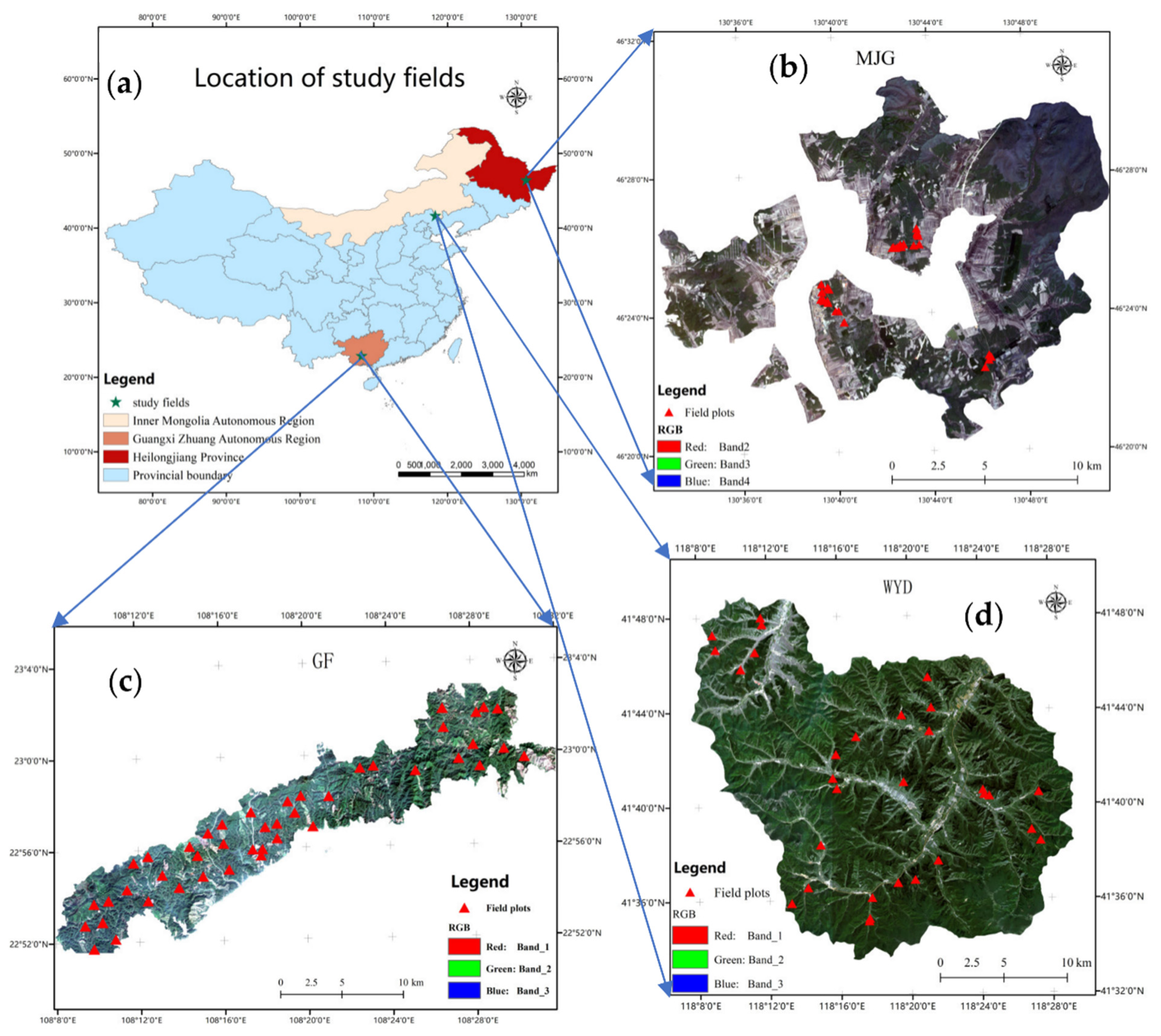
In China, the main forest types include evergreen broadleaf planted forests, deciduous broad-leaved planted forests, evergreen coniferous planted forests, and deciduous needle-leaf planted forests. To enhance the accuracy of the proposed method and to achieve better robustness, research regions that included most of the forest types were selected from around China. The tree species that were planted in these forest farms were also the most commonly planted species in China. The Wangyedian Forest Farm, Gaofeng Forest Farm, and Mengjiagang Forest Farm were chosen for this study because they represent the typical plantation types in the north and south regions of China (Figure 1).

Figure 1.
(a) The location of the study area and the field plots: (b) Mengjiagang Forest Farm (MJG); (c) Gaofeng Forest Farm (GF); (d) Wangyedian Forest Farm (WYD).
The Mengjiagang Forest Farm (MJG) is located in Heilongjiang Province, which is located in the northeast part of China. It is located at 130°32′–130°52′E, 46°20′–46°30′N. The relative height of the mountain on which it is located is 168 to 575 m, and the slope is 10–20°. The total area of the forest farm is 1.7 × 10⁴ km2, and the plantation accounts for 76.7% of the total area and mainly includes larch (Larix gmelinii (Rupr.) Kuzen.), mongolica (Pinus sylvestris var. mongolica Litv.), and Korean pine (Pinus koraiensis Sieb. et Zucc.), with these tree species accounting for about 80% of the plantation population.
The Gaofeng Forest Farm (GF) is located in Guangxi Province, which is located in the south of China. It is located at 108°08′–108°53′E, 22°49′–23°15′N. The forest area is 4.7 × 10⁴ km2, and the forest coverage is 83.7%. The relative height of the mountain on which the forest area is located is 150 to 400 m, and the slope is 20–30°. The forest farm is mainly composed of a secondary plantation. The main tree species are Masson pine (Pinus massoniana Lamb), fir (Cunninghamia lanceolata (Lamb.) Hook.), and fast-growing eucalyptus (Eucalyptusrobusta Smith).
The Wangyedian Forest Farm (WYD) is located in the Inner Mongolia Autonomous Region in the north of China. It is located at 118°09′–118°30′E, 41°35′–41°50′N. The forest area is about 2.5 × 10⁴ km2, and the forest coverage rate is over 80%. The elevation is between 800 m to 1890 m. The relative height of the mountain is around 200 to 400 m and has a slope of 15–35°. The area of the forest farm is composed of 47% planted forest and 53% natural forest, and the main tree species include oil pine (Pinus tabuliformis Carrière) and larch (Larix gmelinii (Rupr.) Kuzen.). Oil pine is present in a proportion of 51%, and the proportion of larch is 47%. The natural forests in this area are mainly composed of white birch (Betula platyphylla), black birch (Betula dahurica), mountain apricot (Armeniaca sibirica), aspen (Populus davidiana), elm (Ulmus pumila), hazelnut (Corylus heterophylla), and other tree species.
2.2. Field Data
A total of 102 plots were set up in the WYD, GF, and MJG. When setting up the plots, it was necessary to ensure that the plots were fully representative of the stand, that they were not scattered across different forest types, and that they were evenly distributed at different levels of the slope and aspect in each forest farm. A total of 30 plots were set up in the WYD with plot areas of 25 × 25 m, of which 18 plots were oil pine forests and 12 were larch forests. Additionally, there were 43 plots in the GF with plot areas of 20 × 20 m, with eucalyptus forests comprising most of the plots. There were 29 plots in the MJG with plot areas of 30 × 20 m. All of the plots were larch forests. The data were normalized to a minimum size of 20 × 20 m to ensure the consistency of the data.
The measured forest parameters included diameter at breast height, tree height, stem height, crown width, and tree species. All of the trees with a diameter at breast height above 5 cm in the plot were measured and recorded in one plot. Then, the GPS coordinates of each plot were recorded. The statistical information of the three research areas can be found in Table 1.

Table 1.
Statistical information regarding the measurements in the three study areas.
The canopy closure, leaf area index (LAI), and clumping index of each plot were measured at the same time. The canopy closure was measured using transects and fisheye camera photos. Two transect lines were laid along the diagonals of the plot, and the vertical projection lengths of the crowns along each transect were recorded. The average ratio of the total projection lengths of the crowns along the two diagonals to the diagonal length was the canopy closure.
The LAI was measured using fisheye camera photos. All of the photos were taken with a Nikon Coolpix 4500. The photos were taken at the four corners and in the center of each plot. The locations in which the images were collected can be found in Figure 2a. The images were analyzed using digital hemispherical photography (DHP). The edges of the photos with large amounts of distortion were removed and processed via binarization. Then, the canopy pixel value was recorded as 1, the gap was recorded as 0, and the ratio of the number of pixels with a value of 1 to the total number of pixels was the canopy closure. Finally, the average canopy closure of the five images was the canopy closure of the plot obtained using the fisheye camera method. At the same time, the effective LAI was also able to be automatically calculated using DHP. Details of this method can be found in [62].

Figure 2.
(a) The location of the fisheye camera photographs in one plot; (b) a sample of a fisheye camera photo; (c) a scene from the field measurements.
The clumping index of each plot was measured by using a TRAC instrument. Two line transects that were 20 m in length were measured. Then, the TRAC-based PPFD gradient values along the transects perpendicular to the incident directions of the solar beams were collected. In the end, the clumping index of each plot was calculated using TRACWin software. Details can be found in [63].
2.3. Methods
2.3.1. The GOST Model and Canopy Gap Fraction Simulation
The GOST model is a geometric-optical model for sloping terrains developed based on the four-scale model [64]. The four-scale model is one of the most popular geometric-optical models and can be used to simulate the bidirectional reflectance distribution function of forest canopies on flat surfaces [65]. By considering the structure of the canopy at four scales, viz., tree groups, tree crowns, branches, and shoots, the bidirectional reflectance characteristics of the forest canopies can be simulated. The four-scale model defines how the canopy reflectance in one pixel is a linear combination of the signals from four components: the sunlit and shaded foliage and the sunlit and shaded backgrounds. The total canopy reflectance is as follows:
where is the reflectivity of the sunlit foliage; is the reflectivity of the sunlit background; is the reflectivity of the shaded foliage, is the reflectivity of the shaded background; , , , and are the sensor-viewing probabilities of the four scene components, respectively (Figure 3).
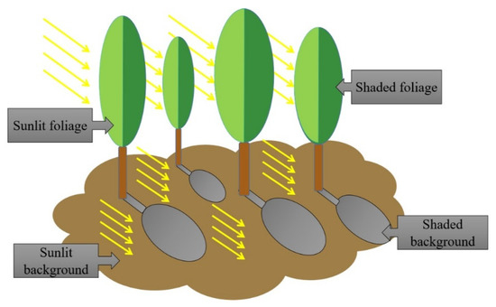
Figure 3.
Schematic illustration of sunlit foliage and background and shaded foliage and background.
In the four-scale model, the probability of seeing the ground represents the ground that can be seen between tree crowns. It is a function of the projected tree crown area and the spatial distribution characteristics of trees in a quadrat. It can be calculated as follows, based on the method in [65]:
where Pvg-c is the probability of seeing the ground, i is the number of trees in a region with the area A, and is the ground surface not seen by the viewer because of one tree. is the probability of having i trees in A, and it is determined by the Neyman distribution. In this equation, the tree crowns are assumed to be opaque, and the gaps within the tree crowns are not considered.
If the gaps in the crowns and the overlaps in the crowns are considered, then Equation (2) can be written as follows:
where
This is the gap probability inside the trees.
The gap probability . is calculated based on the method developed by Li and Strahler [53], but the foliage clumping effect is considered in the four-scale model. . is the function of the foliage angle distribution = 0.5 [65] in this research. L0 is the LAI. . is the clumping index of the shoots within the tree crowns. is the ratio of the needle to shoot area.
In Equation (2), is the probability of having j trees intercepting the view line. Additionally, it can be calculated using a negative binomial function.
In the case of j = 0, is equal to Equation (2).
The canopy gap fraction determines the contribution of the under surface to the reflectance measured above the canopy. Additionally, the canopy gap fraction can be calculated using the tree crown projection made on the ground surface. It is based on the method described above for calculating the shadow area. After calculating the shadow area projected by a single tree onto the ground, the sunlit crown proportion seen by the viewer can be computed using the total surface area of the tree visible to the viewer projected to a plane perpendicular to the view line. It is not difficult to determine that the canopy gap fraction is highly related to canopy closure according to the method in the four-scale model.
In addition, topography is an important factor that has a serious effect on the bidirectional reflectance distribution function of forest canopies. Therefore, in order to make the four-scale model more suitable to simulate the bidirectional reflectance distribution function of the forest canopies on slopes, the GOST model, which is a geometric-optical model that considers the oblique topographical factors, was used in this study [64].
The GOST model was used to simulate the canopy reflectance for two different gap fractions. In one case, the gap fraction (Pvg-c) was calculated by Formula (2) during the assumption of the opaque canopy bodies. In the other case, the gap fraction (Pvg) was calculated using Formula (3), and gaps and overlaps were observed in the crowns. The output of the GOST model was the canopy reflectance and probability of seeing the four scene components under different view angles (Equation (1)). The four components were the sunlit foliage, the sunlit ground, the shaded foliage, and the shaded ground, and the mixed pixel decomposition problem was able to be solved as well. A database of the reflectance under various gap fractions was established, allowing the relationships between the canopy gap fraction and the stand canopy closure to be discussed. When the canopy was an opaque body, the estimated canopy closure was the true stand canopy closure, and the canopy closure measured by the traditional transects was used to verify the estimated results. When the gaps in the crowns were considered, the estimated canopy closure was compared to those measured results obtained via fisheye camera photos. This study discusses the feasibility of estimating the canopy closure using the GOST model and the spatial resolution effects of the remote sensing images.
2.3.2. Canopy Closure Estimation Based on the GOST Model
The GOST model was selected and used to simulate the canopy reflectance for a complex canopy structure. When the canopy reflectance was able to be estimated accurately, it was found to be closely related to the gap fraction function. This was because the canopy gap fraction was used to describe the light passing through the canopy. As such, the canopy gap fraction can describe canopy closure. A higher canopy gap fraction means less canopy closure, and vice versa. Additionally, it is also the reason why the canopy gap fraction can be used to estimate the canopy closure.
Two gap fractions were included in the GOST model. In one case, the canopy was assumed to be an opaque canopy body. Additionally, the gaps within the tree crown were not considered. Since canopy closure does not consider the gaps in the canopy, if the viewing direction was vertical, then the gap fraction of the viewing canopy gap fraction is the percentage of light passing through the canopy and projected to the ground surface. Additionally, the stand canopy closure should be 1 − Pvg-c.
where is the canopy closure of the opaque canopy bodies and is the gap fraction of the opaque canopy bodies.
In the other case, the gap fraction was assumed to be a tree crown with gaps. Generally, it was assumed that there were gaps in the canopy for the canopy closure values that were obtained by the fisheye camera images or estimated from the remote sensing data; therefore, the estimated canopy closure should be 1 − Pvg. As such, the canopy closure could be calculated as follows:
where and were the canopy closure and gap fraction when there were tree crown gaps, respectively.
The input parameters of the GOST model were determined to be , and then the Pvg-c and Pvg could be simulated under various input parameters using the GOST model, and the database for the Pvg-c and Pvg and the input parameters was established. The relationships among the Pvg-c, Pvg, and the inputs were able to be established using a statistical method.
where and were the functions of the Pvg-c and related inputs, respectively. Once the relationship between the gap fraction and the inputs was established, then the gap fraction could be estimated, and the canopy closure was able to be inverted based on Equations (7) and (8).
2.3.3. Sensitivity Analysis of the GOST Model Parameters
Geometric-optical models have a large number of input variables, but we only need to know the key input variables. It is crucial to carry out a sensitivity analysis on the parameters for simulation in a complex model, especially for a model with multiple input parameters. The inputs of the GOST model included plot parameters (size of plot, number of trees in plot, LAI, slope, aspect, solar zenith angle, solar azimuth angle, view zenith angle, view azimuth angle), tree structural parameters (radius of the crowns, stem height, crown height, half apex angle, clumping index for shoots in the crown), and spectral parameters (leaf reflectivity, leaf transmittance, and ground reflectance). Therefore, the sensitivity analysis was an important process in this study. The function (Equation (11)) of the sensitivity analysis was used to determine the sensitivity of the inputs affecting the gap fraction of the canopy. It was very helpful to improve the accuracy and robustness of the model for the canopy closure estimation [66,67].
where is the Pvg-c, and Pvg is calculated based on the measured parameters (reference). is the Pvg-c and Pvg when the parameter was disturbed, and is the sensitivity of the input parameters [68].
The sensitivity of the tree structure parameters, leaf reflectivity, leaf transmittance, and ground reflectivity was analyzed in this study. Additionally, the topography effects were corrected in the GOST model, so there was no need for a slope sensitivity analysis.
According to the results of the sensitivity analysis, the input parameter dataset, which was sensitive to canopy closure, was determined as . The insensitive inputs were set as the average values of the measurements in the plot. Then, the Pvg-c and Pvg were able to be simulated under various input parameters using the GOST model, and the database between the Pvg-c and Pvg and the input parameters was established. The relationship between the Pvg-c, Pvg, and the inputs was able to be established, and the canopy closure could then be inverted based on Equations (7) and (8).
2.3.4. Validation
In this study, the R2 and RMSE were selected to evaluate the precision of the canopy closure estimation model. These were calculated using Equations (12) and (13).
where was the measured value of the sample , was the predicted value of the sample , was the average of all the samples, and was the number of samples.
3. Results
3.1. Results of Sensitivity Analysis of the Parameters in the GOST Model
Since the canopy closure was the ratio of the vertical projection area of the crowns to the area of forest land and was not affected by the slope, the incident angle of the view direction was equal to 0 degrees. Without considering the influence of the slope, the sensitivity of the slope was 0. The sensitivity of the radius of the crown, stem height, crown height, half apex angle, clumping index for shoots in the crown, shape of crown, LAI, tree number, leaf reflectivity, leaf transmittance, ground reflectivity, solar azimuth angle, and view azimuth angle were calculated, and the results are shown in Table 2.

Table 2.
Sensitivity analysis of the parameters in the GOST model.
The radius of the crown and the number of plants had a greater influence on the Pvg-c (the gap fraction between the crowns), and the other parameters had no influence. This was because the canopy was considered to be an opaque canopy. Additionally, the canopy closure was only affected by the radius of the crown and individual trees, and it was not related to the leaf area index and clumping index. Therefore, when the radius of the crown and the number of trees were determined, the vertical projection area of the canopy on the forest could be estimated. However, when the gaps in the crown were considered, the LAI had the greatest effect on the Pvg (total gap fraction of the canopy). The clumping index had the next largest effect, followed by the radius of the crown and the number of trees.
3.2. Estimation of the Canopy Gap Fraction Based on the GOST Model
The results of the parameter sensitivity analysis show that the number of trees (n), radius of the crown (d), and LAI (l) had a greater impact on Pvg-c and Pvg simulation. While n, d, and l were set as the measured values, other insensitive parameters were set as the average value of all of the sample plots. Then, the Pvg-c and Pvg of all of the plots were simulated by the GOST model. The max of the simulated Pvg-c was 0.6671, the min value of the Pvg-c was 0.2051, and the mean value was 0.4589. Additionally, the max, min, and mean values of the Pvg were 0.7439, 0.3011, and 0.5641, respectively. Additionally, the value of Pvg-c was obviously smaller than the simulated Pvg value.
When the Pvg-c and Pvg of all of the plots were simulated, the relationship between the Pvg-c and Pvg and the field-measured data was analyzed. In our statistical analysis, we found that the linear relationships among the Pvg-c and Pvg and the single parameters of the number of trees and the radius of the crown were quite insignificant, respectively. In contrast, this combination of n × d2 variables had a better linear relationship with the canopy gap fraction. Additionally, the n × d2 variable was a variable because it represented the projected area of the forest canopy and was physically significant for Pvg-c and Pvg estimation compared to the single variables d or n.
As such, the relationships among the Pvg-c, Pvg, and n × d2 were established (Table 3). The established models passed the significance test.

Table 3.
Statistical models of Pvg and Pvg-c estimation using n × d2.
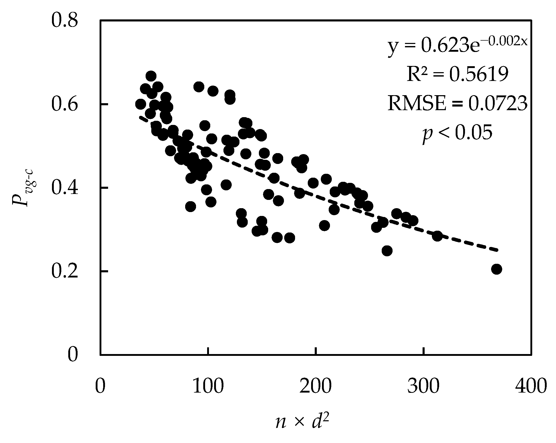
The results show that the linear relationship between n × d2 and the Pvg-c was significant, with the coefficient of determination being 0.5619 (Figure 4). Additionally, the reason for this could be that the Pvg-c only considered the gaps between the canopies and ignored the gaps in the crown. The variable n × d2 represented the projected area of all of the canopies in the plot, taking the canopy as an opaque body without considering the gaps in the crown. Therefore, n × d2, which represents the projected area of the forest canopy, can describe the canopy closure well. Therefore, the linear relationship between n × d2 and the Pvg-c was more significant, and the coefficient of determination was larger than the one in Table 3.

Figure 4.
Scattering plot between Pvg-c and n × d2.
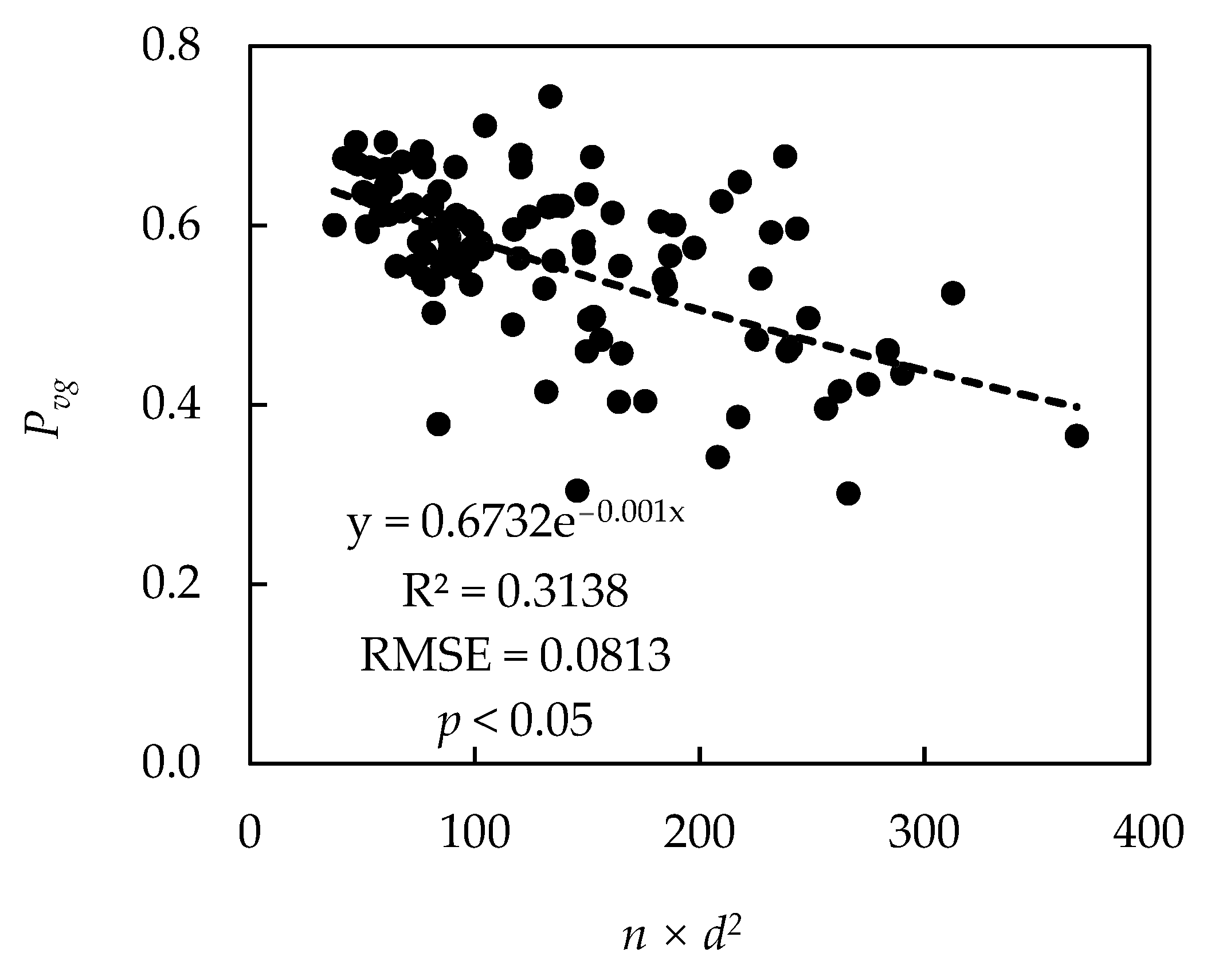
The relationship between n × d2 and the Pvg can be seen in Figure 5. The coefficient of determination and the RMSE of the canopy closure estimation model were 0.3138 and 0.0813, respectively. Compared to the model established with the Pvg-c, these results do not seem to be as good as the results above. This is because the gap between the canopy was represented by the Pvg in the GOST model. Additionally, n × d2 represented the projections of the canopy without considering the gaps in the canopy. Therefore, the linear relationship between these two variables was weakened. At the same time, the results that were estimated using this model underestimate the canopy due to the gaps in the canopy represented by the Pvg.
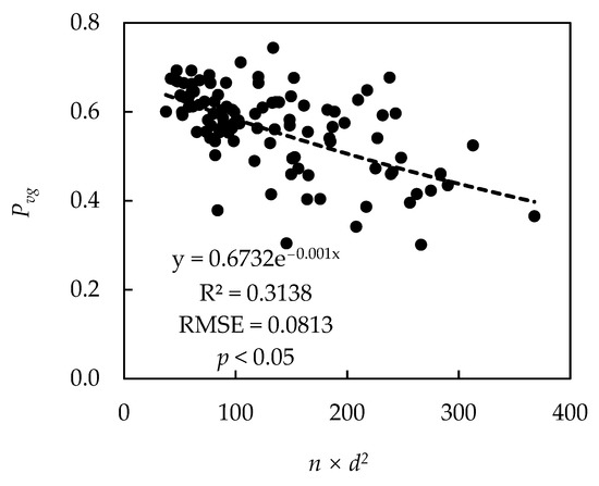
Figure 5.
Scattering plot between Pvg and n × d2.
3.3. Estimation of the Canopy Gap Fraction Based on the LAI
The canopy gap fraction can be estimated based on the number of trees and the radius of the crown. However, it was difficult to estimate the number of trees and the radius of the crown from most of the middle-resolution remote sensing data, and it turned out to be impossible. To solve this shortage, the LAI was used to solve this problem. Based on the equation to calculate the canopy gap fraction (Equation (5)), the LAI had a significant relationship with the canopy gap fraction. Additionally, the LAI was a key parameter for solving this problem. The LAI is a commonly used forest structural parameter, and there are many LAI estimation methods that are highly accurate [69,70]. This means that the LAI can be obtained from remote sensing images easily and that it can be used to estimate the canopy closure for middle-resolution remote sensing images. The relationships among the Pvg-c, Pvg, and LAI (l) were established and are shown in Table 4. These models passed the significance test.

Table 4.
Statistical models of Pvg and Pvg-c estimation using the LAI.
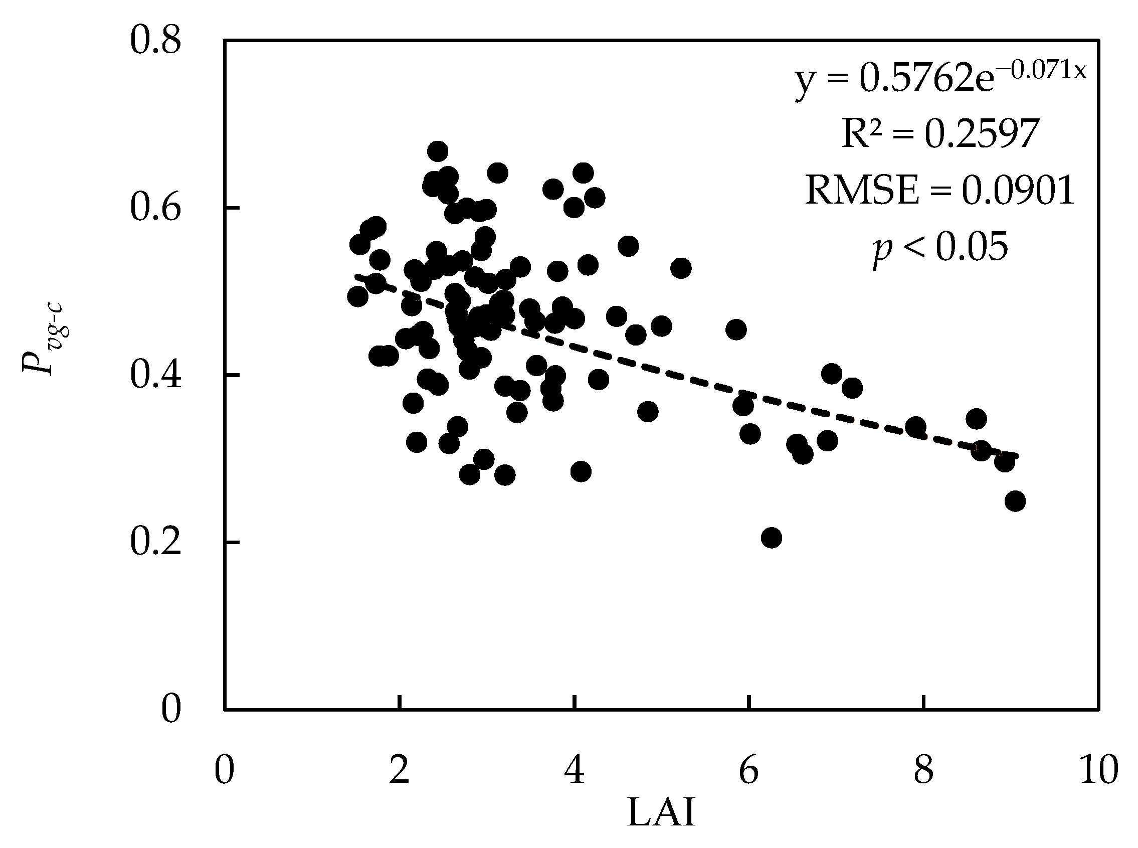
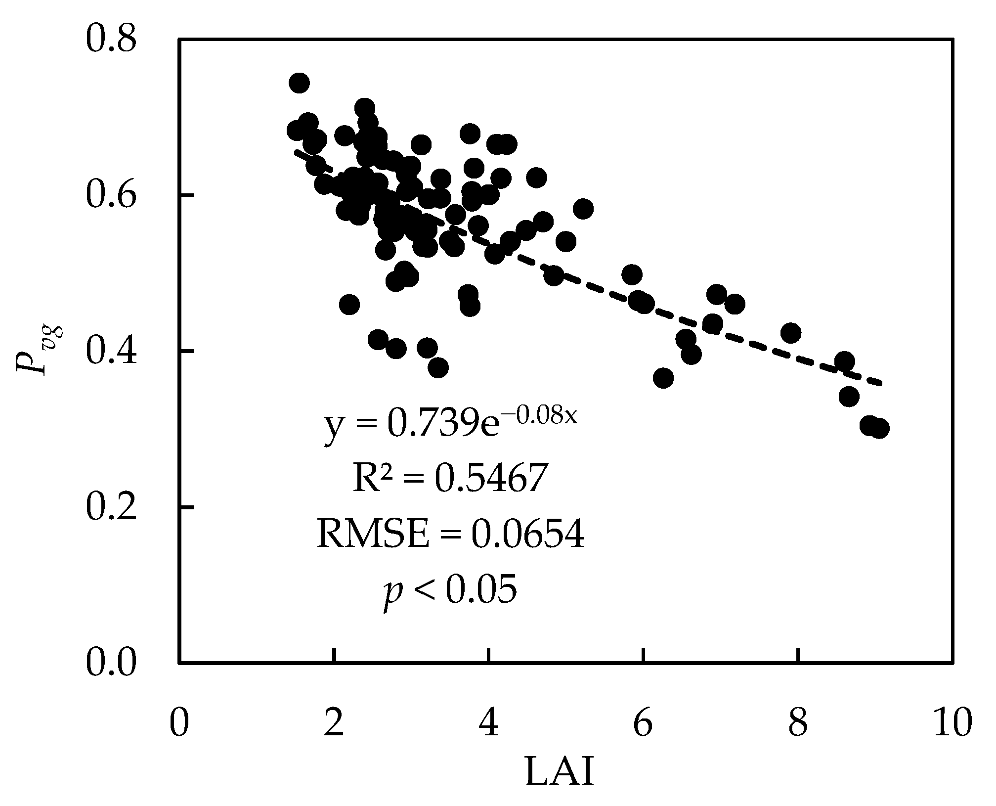
The results show that the linear relationships among the Pvg-c, Pvg, and LAI were significant, with the coefficients of determination being 0.2597 and 0.5467, respectively (Table 4). An exponential function between the Pvg-c and LAI was observed, with the coefficient of determination being 0.2597, shown in Figure 6. Although this model passed the significance test, the accuracy of the simulation was not as good as expected. Additionally, these fitting results are also not as good as the results that were obtained using the variable n × d2.
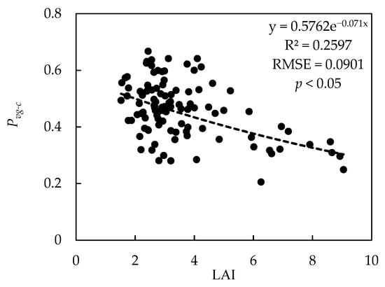
Figure 6.
Scattering plot between Pvg-c and LAI.
The linear relationship between the Pvg and LAI was significant, with the coefficients of determination being 0.5467 and RMSE of 0.0654, respectively (Table 4). An exponential function between the Pvg and LAI is also visible in Figure 7. These results are consistent with Equation (5), but the relationship between the gap fraction and the LAI was affected by other parameters of Equation (5). The reason for this is that the real exponential function was not as significant as Equation (5). In addition, compared to the results of the Pvg-c, the Pvg had a better linear relationship with the LAI. This could be related to the LAI, which was defined as half of the total leaf area of all of the canopies in the plot per unit of ground area [71]. As such, the gaps in and between the canopies were considered. Therefore, the linear relationship between the Pvg and the LAI was better than that between the Pvg-c and the LAI. At the same time, compared to the variable n × d2, the LAI was more suitable for Pvg estimation, achieving R2 and RMSE values of 0.5467 and 0.0654, respectively.
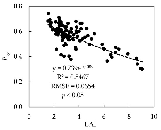
Figure 7.
Scattering plot between Pvg and LAI.
3.4. Verification of Estimation of Canopy Closure Based on Pvg-c
Based on the definition of canopy closure, only the gaps between the canopies were considered, so the value of 1 − Pvg-c should be equal to the canopy closure. A linear regression model was established between the canopy closure and 1 − Pvg-c. The R2 and RMSE values were 0.5216 and 0.0832, respectively (Figure 8), and the precision of the canopy closure estimation was 86.69%. At the same time, the established model passed the significance test. It can be seen that the canopy closure measured by the line transects had a significantly good relationship with 1 − Pvg-c. Among the traditional methods for measuring canopy closure, the line transect method was more accurate. Therefore, it was very effective and feasible to estimate canopy closure using the GOST model.
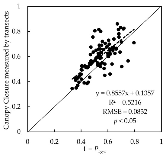
Figure 8.
Scattering plot between the measured canopy closure and 1 − Pvg-c (the black solid line is y = x).
3.5. Verification of the Estimation of the Canopy Closure Based on Pvg
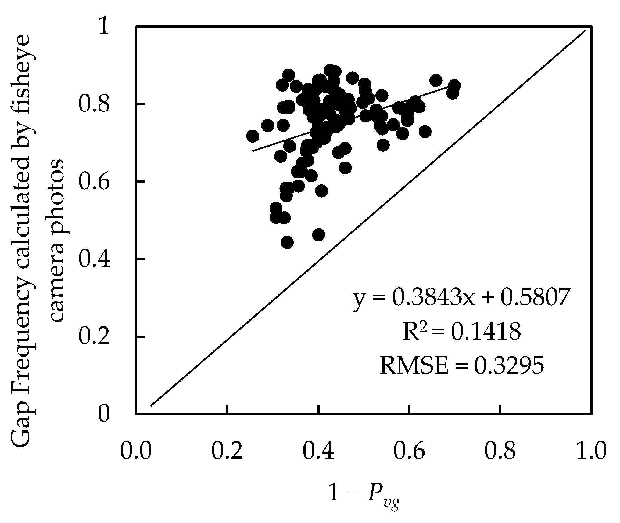
The canopy closure calculated based on the fisheye camera photos included the gaps in the canopy. Therefore, calculating the canopy closure using the fisheye camera photos can verify the canopy closure estimated based on the Pvg. The R2 and RMSE values of the linear regression model were 0.1418 and 0.3295, respectively (Figure 9). The average accuracy of the canopy closure estimation was 73.2%. The model also passed the significance test. The results show that the relationship does not appear to be good. This could be because the fisheye camera images were taken at a 180 degree angle, resulting in the deformation increasing as the view angle became larger, while the GOST model calculated the Pvg when the view angle was 90 degrees [72]. The reason for this was that the projected area of the crown between these two styles was different, so the linear relationship was not as significant.

Figure 9.
Scatter plot between canopy closure measured by fisheye camera images and 1 − Pvg.
4. Discussion
Canopy closure is a multipurpose ecological indicator that is used to assess the light conditions and forest floor microclimate as well as to distinguish types of plant and animal habitats [13]. Canopy closure also determines light interception and is crucial for understanding forest carbon fixation and responses and feedback to climate change [73]. Unfortunately, the in situ measurement of canopy closure is a time-consuming and laborious process, whilst advances in non-destructive, indirect techniques have been made [15]. Indirect optical methods derive canopy closure by measuring the canopy gap fraction or via transmittance [74]. These in situ measurements are able to capture the canopy at the plot (and site) scale, but these methods cannot adequately characterize spatiotemporal dynamics [32].
More and more remote sensing applications involve the estimation of canopy closure. The least squares method is one of the most commonly used methods for canopy closure estimation. However, the linear relationship is data dependent. This means that accuracy will be affected by the data quality and that applications will be limited by the area of the research region [75]. Other studies have used the random forest and Cubist models to estimate the canopy closure. However, the precision of these models is not accurate enough because a single variable is used for regression analysis [10]. In contrast, non-parametric models have always had better estimation results, and the accuracy of the modeling and estimation would be limited by the number of the samples, as small samples weaken the predictive ability of the model [76,77]. To make up for these shortages, we established a canopy closure estimation method that uses the gap fraction based on the geometric-optical GOST model, and the results were discussed.
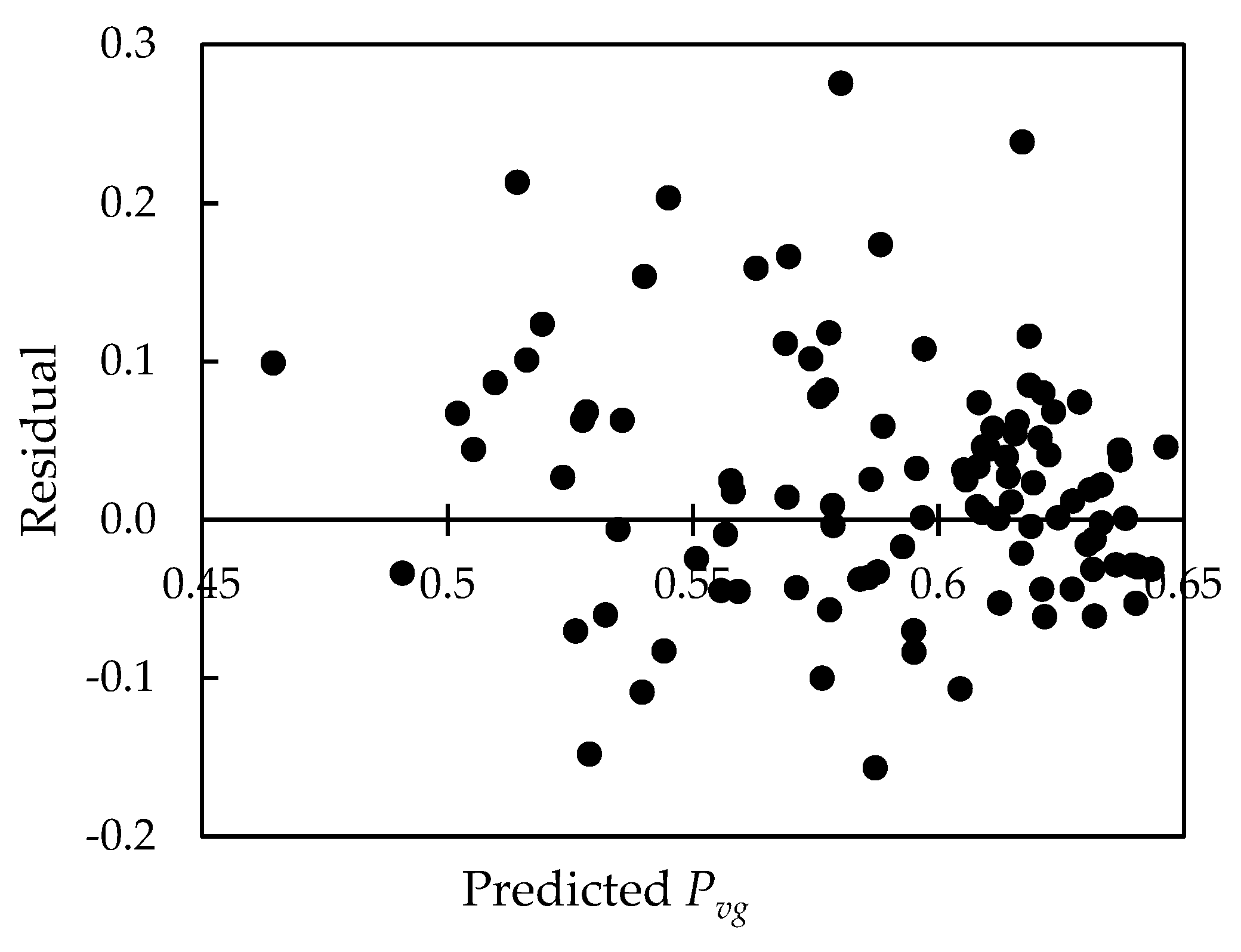
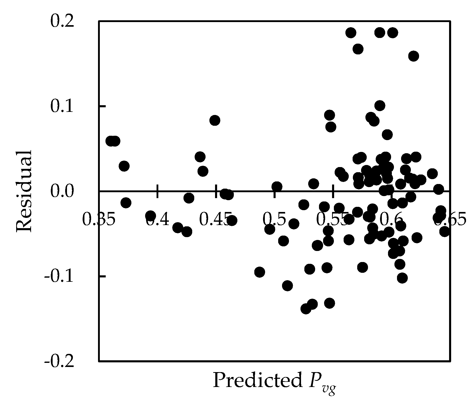
A canopy closure estimation method that uses the gap fraction was represented in this study. The canopy closure Pvg-c was highly correlated with the average projected area of the canopy. The Pvg-c was estimated based on the number of plants in the plot and the average radius of the crowns, and the accuracy of the estimated canopy closure was 86.69%, while the accuracy of the canopy closure estimated by the Pvg was 7%. In the residual analysis of the canopy closure model, the Pvg-c, Pvg, and n × d2 (Figure 10 and Figure 11) show that the residuals of the two models were distributed within a reasonable range and relatively evenly. The results show that the accuracy of the Pvg-c estimation of the model was higher than that of the residual plots for Pvg-c and n × d2. The residuals were distributed between ±0.2. However, the Pvg was not estimated as well as the Pvg-c was (Figure 11). The residuals of the Pvg were distributed between −0.2 and 0.3. It can be seen that estimating the canopy closure Pvg-c between the canopies using the number of plants and the average radius of the crowns produced better results.
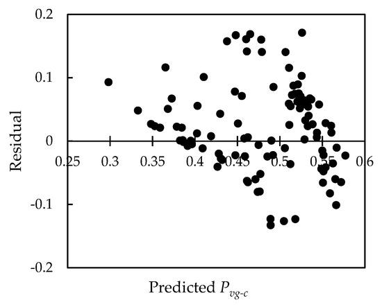
Figure 10.
The residual plot of the estimated Pvg-c and n × d2.
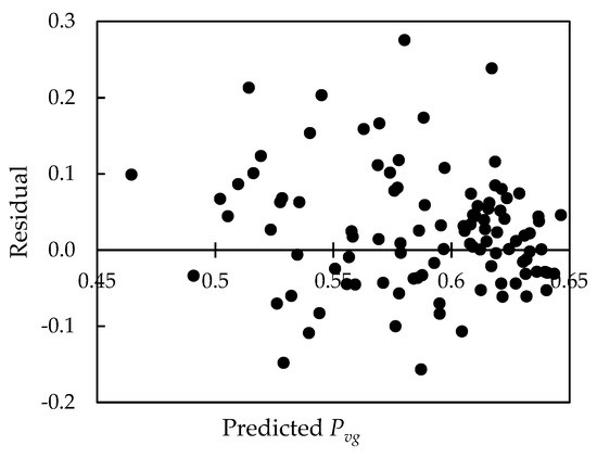
Figure 11.
The residual plot of the estimated Pvg and n × d2.
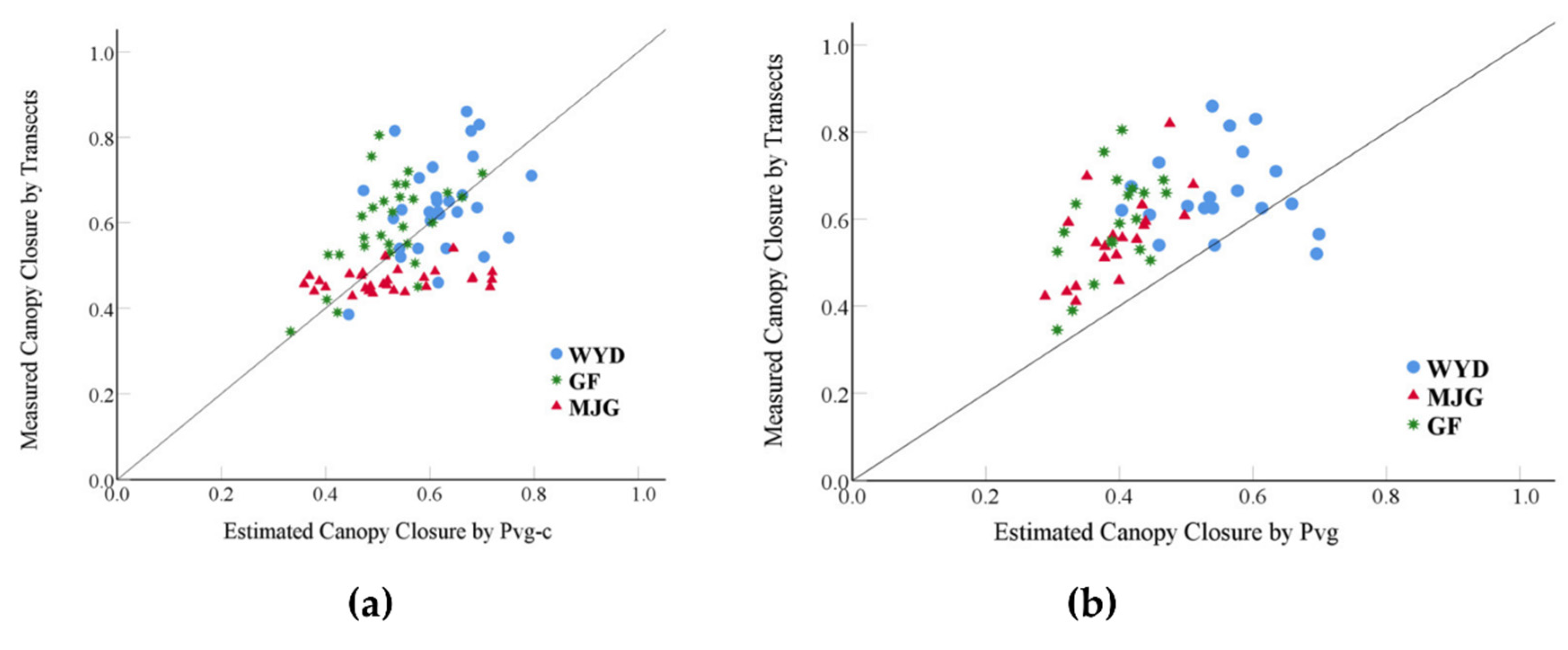
For most of the remote sensing images with a high spatial resolution, the number of plants and the radius of the crown were able to be extracted easily by means of image segmentation technology, and the parameters of these two variables can be considered an approach to canopy closure estimation using remote sensing images with a high spatial resolution. The relationship between the Pvg-c and n × d2 was the best optimal method, obtaining high-precision canopy closure estimation results. The line transect method was more accurate compared to other methods. As such, the scattering plot for the estimated canopy closure determined and measured by the gap fraction can be found in Figure 12. The canopy closure that was estimated by the Pvg-c was consistent with the measured canopy closure. However, the canopy closure that was estimated by the Pvg deviated from the line y = x. Additionally, the canopy closure was underestimated.
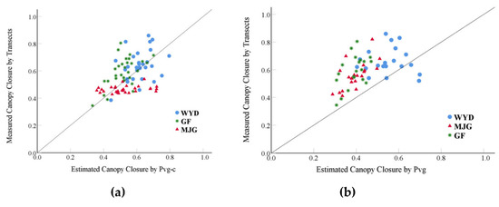
Figure 12.
(a) The scattering plot of the canopy closure measured and estimated by Pvg-c; (b) the scattering plot of the canopy closure measured and estimated by Pvg.
Compared to traditional statistical models, the model in the present study was not affected by the study area or the dataset, and there was no need to establish models in different study areas. The canopy closure estimation method simulated the probability of being able to see the ground by considering the mechanism of the light transmission process in the canopy and the gaps or opaque canopy in the viewing direction, which can also be considered individually using the geometric-optical model (the GOST model), and the estimated results also have high accuracy. In other words, this means that this estimated method was more robust compared to statistical methods. If remote sensing data with medium or low spatial resolution are used, then the parameters used for canopy estimation cannot be inverted accurately because of the mixed pixel effect [44]. Additionally, most of the parameters, such as the number of the trees and the radius of the crown could be obtained, so this method was difficult to implement. Instead, some medium-level variables, such as the LAI, should be used for canopy closure estimation even though the accuracy varies from study to study [78,79,80,81,82]. In this study, we evaluated the canopy closure estimation efficiency when using the LAI. The values of the residuals were more discrete from the residual Pvg-c and LAI plots (Figure 13). Additionally, the figure shows that the accuracy of the Pvg-c estimation was better when the canopy closure was greater than 0.4 and when the value of residuals was lower than 0.1. When the canopy closure was greater than 0.4, the accuracy of the Pvg-c prediction was obviously lower.
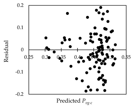
Figure 13.
The residual plot of the estimated Pvg-c and LAI.
The situation with the Pvg was similar to that of the Pvg-c. The residuals of the Pvg became significantly discrete from the residual Pvg and LAI plots when the canopy closure was larger than or less than 0.45 (Figure 14). The most possible reason for this is that more gaps in the crown could be detected when using remote sensors with a low or medium spatial resolution, and the efficiency of the mixed pixels enhanced the signals of the forest floor or those of other features. Inversely, the larger amount of canopy closure meant smaller gaps in the crown, and the detected probability of the signal outside of the canopy was lower compared to larger gaps, weakening the mixed pixel effect. As such, it was necessary to consider the efficiency of the mixed pixels in the images when the LAI was used to estimate the canopy closure. In comparison, a geometric-optical model was used to decompose the mixed pixels into four components, allowing the forest components in the pixels to be more accurately distinguished. That was the advantage of the method using a physical model. At the same time, the physical canopy closure estimation procedure using a geometric-optical model was clearer than the traditional statistical model or the pixel binary model, and the robustness and accuracy of the model were self-evident. In addition, the results also indicate that the LAI can be used to estimate the Pvg with good accuracy. Once high-quality LAI data were obtained, the canopy closure could also be estimated, especially for remote sensing images with a medium or low spatial resolution. This method provided a way to estimate the canopy closure using the LAI. Additionally, this relationship was derived from geometric-optical models and was not data dependent, which is the case using statistical theory. Additionally, this method can effectively avoid the shortcomings of canopy estimation models that are based on statistical methods.

Figure 14.
The residual plot of the estimated Pvg and LAI.
5. Conclusions
Canopy closure is an important forest inventory parameter, and it plays an important role in forestry production and management and forest health evaluation. In this study, the GOST model was used to simulate the characteristics of forest canopy gap fractions by considering an opaque canopy (Pvg-c) and gaps in the tree crown (Pvg). Additionally, exponential models for estimating the canopy closure of a plantation based on the gap fraction were established. The results show the following:
- (1)
- It was feasible to estimate canopy closure based on the GOST model, and the feasible method was proved with sample data measured from three different regions in China.
- (2)
- Compared to the LAI, n × d2 had a better relationship with the gap fractions simulated using the GOST model. Therefore, when remote sensing images or LiDAR data of the study area with high spatial resolution were available, the crown recognition method could be used to obtain the number of plants and the average radius of the crowns in the plot, so the gap fraction Pvg-c and the forest canopy closure could be accurately estimated and predicted in the research area.
- (3)
- When the number of plants and the average radii of the crowns in the plot could not be extracted using remote sensing images, especially when only medium- or low-spatial resolution remote sensing data were available, the LAI, a medium parameter, could be used to estimate the canopy closure with an acceptable level of accuracy. This also provided a new a canopy closure estimation approach using medium- or low-spatial resolution remote sensing data. This study can provide a reference for canopy closure estimation using geometric-optical models.
Author Contributions
Y.Y. conceptualized and designed the experiments; P.H. performed the experiments and analyzed the data; X.Y. and P.H. wrote the paper; X.Y., Y.Y. and W.F. reviewed and edited the paper. All authors have read and agreed to the published version of the manuscript.
Funding
This research was funded by the National Natural Science Foundation of China, grant numbers: 31870621 and 31971580; the Fundamental Research Funds for the Central Universities of China, grant numbers: 2572021BA08, 2572019BA10, and 2572019CP12; the China Postdoctoral Science Foundation, grant number: 2019M661239; National Forestry and Grassland Data Center-Heilongjiang platform, grant number: 2005DKA32200-OH.
Conflicts of Interest
The authors declare no conflict of interest.
References
- Payn, T.; Carnus, J.-M.; Freer-Smith, P.; Orazio, C.; Nabuurs, G.-J. Third International Congress on Planted Forests: Planted Forests on the Globe-Renewable Resources for the Future. N. Z. J. For. Sci. 2014, 44, S1. [Google Scholar] [CrossRef]
- Payn, T.; Carnus, J.-M.; Freer-Smith, P.; Kimberley, M.; Kollert, W.; Liu, S.; Orazio, C.; Rodriguez, L.; Silva, L.N.; Wingfield, M.J. Changes in planted forests and future global implications. For. Ecol. Manag. 2015, 352, 57–67. [Google Scholar] [CrossRef]
- Buongiorno, J.; Zhu, S. Assessing the impact of planted forests on the global forest economy. N. Z. J. For. Sci. 2014, 44, S2. [Google Scholar] [CrossRef]
- Brockerhoff, E.G.; Jactel, H.; Parrotta, J.A.; Ferraz, S.F.B. Role of eucalypt and other planted forests in biodiversity conservation and the provision of biodiversity-related ecosystem services. For. Ecol. Manag. 2013, 301, 43–50. [Google Scholar] [CrossRef]
- Gschwantner, T.; Schadauer, K.; Vidal, C.; Lanz, A.; Tomppo, E.; di Cosmo, L.; Robert, N.; Duursma, D.E.; Lawrence, M. Common tree definitions for national forest inventories in Europe. Silva Fenn. 2009, 43, 303–321. [Google Scholar] [CrossRef]
- Jennings, S.B.; Brown, N.D.; Sheil, D. Assessing forest canopies and understorey illumination: Canopy closure, canopy cover and other measures. Forestry 1999, 72, 59–74. [Google Scholar] [CrossRef]
- IPCC. Good Practice Guidance for Land Use, Land-Use Change and Forestry; Institute for Global Environmental Strategies (IGES): Hayama, Japan, 2003. [Google Scholar]
- Xu, B.; Gong, P.; Pu, R. Crown closure estimation of oak savannah in a dry season with Landsat TM imagery: Comparison of various indices through correlation analysis. Int. J. Remote Sens. 2003, 24, 1811–1822. [Google Scholar] [CrossRef]
- Hua, Y.; Zhao, X. Multi-Model Estimation of Forest Canopy Closure by Using Red Edge Bands Based on Sentinel-2 Images. Forests 2021, 12, 1768. [Google Scholar] [CrossRef]
- Chen, G.; Lou, T.; Jing, W.; Wang, Z. Sparkpr: An Efficient Parallel Inversion of Forest Canopy Closure. IEEE Access 2019, 7, 135949–135956. [Google Scholar] [CrossRef]
- Smith, A.M.; Ramsay, P.M. A comparison of ground-based methods for estimating canopy closure for use in phenology research. Agric. For. Meteorol. 2018, 252, 18–26. [Google Scholar] [CrossRef]
- Fiala, A.C.S.; Garman, S.L.; Gray, A.N. Comparison of five canopy cover estimation techniques in the western Oregon Cascades. For. Ecol. Manag. 2006, 232, 188–197. [Google Scholar] [CrossRef]
- Korhonen, L.T.; Korhonen, K.; Rautiainen, M.; Stenberg, P. Estimation of forest canopy cover: A comparison of field measurement techniques. Silva Fenn. 2006, 40, 577–588. [Google Scholar] [CrossRef]
- Paletto, A.; Tosi, V. Forest canopy cover and canopy closure: Comparison of assessment techniques. Eur. J. For. Res. 2009, 128, 265–272. [Google Scholar] [CrossRef]
- Brown, L.A.; Ogutu, B.O.; Dash, J. Tracking forest biophysical properties with automated digital repeat photography: A fisheye perspective using digital hemispherical photography from below the canopy. Agric. For. Meteorol. 2020, 287, 107944. [Google Scholar] [CrossRef]
- Macfarlane, C.; Hoffman, M.; Eamus, D.; Kerp, N.; Higginson, S.; McMurtrie, R.; Adams, M. Estimation of leaf area index in eucalypt forest using digital photography. Agric. For. Meteorol. 2007, 143, 176–188. [Google Scholar] [CrossRef]
- Vales, D.J.; Bunnell, F.L. Comparison of methods for estimating forest overstory cover. I. Observer effects. Can. J. For. Res. 1988, 18, 606–609. [Google Scholar] [CrossRef]
- Li, J.; Mao, X. Comparison of Canopy Closure Estimation of Plantations Using Parametric, Semi-Parametric, and Non-Parametric Models Based on GF-1 Remote Sensing Images. Forests 2020, 11, 597. [Google Scholar] [CrossRef]
- Chopping, M.; Moisen, G.G.; Su, L.; Laliberte, A.; Rango, A.; Martonchik, J.V.; Peters, D.P.C. Large area mapping of southwestern forest crown cover, canopy height, and biomass using the NASA Multiangle Imaging Spectro-Radiometer. Remote Sens. Environ. 2008, 112, 2051–2063. [Google Scholar] [CrossRef]
- Smith, A.M.S.; Falkowski, M.J.; Hudak, A.T.; Evans, J.S.; Robinson, A.P.; Steele, C.M. A cross-comparison of field, spectral, and lidar estimates of forest canopy cover. Can. J. Remote Sens. 2009, 35, 447–459. [Google Scholar] [CrossRef]
- Hill, M.J.; Román, M.O.; Schaaf, C.B.; Hutley, L.; Brannstrom, C.; Etter, A.; Hanan, N.P. Characterizing vegetation cover in global savannas with an annual foliage clumping index derived from the MODIS BRDF product. Remote Sens. Environ. 2011, 115, 2008–2024. [Google Scholar] [CrossRef]
- Chopping, M.; North, M.; Chen, J.; Schaaf, C.B.; Blair, J.B.; Martonchik, J.V.; Bull, M.A. Forest Canopy Cover and Height from MISR in Topographically Complex Southwestern US Landscapes Assessed with High Quality Reference Data. IEEE J. Sel. Top. Appl. Earth Obs. Remote Sens. 2012, 5, 44–58. [Google Scholar] [CrossRef]
- Tuominen, S.; Pekkarinen, A. Local radiometric correction of digital aerial photographs for multi source forest inventory. Remote Sens. Environ. 2004, 89, 72–82. [Google Scholar] [CrossRef]
- Lisein, J.; Pierrot-Deseilligny, M.; Bonnet, S.; Lejeune, P. A Photogrammetric Workflow for the Creation of a Forest Canopy Height Model from Small Unmanned Aerial System Imagery. Forests 2013, 4, 922–944. [Google Scholar] [CrossRef]
- Navarro, J.A.; Tomé, J.L.; Marino, E.; Guillén-Climent, M.L.; Fernández-Landa, A. Assessing the transferability of airborne laser scanning and digital aerial photogrammetry derived growing stock volume models. Int. J. Appl. Earth Obs. Geoinf. 2020, 91, 102135. [Google Scholar] [CrossRef]
- Edson, C.; Wing, M.G. Airborne Light Detection and Ranging (LiDAR) for Individual Tree Stem Location, Height, and Biomass Measurements. Remote Sens. 2011, 3, 2494–2528. [Google Scholar] [CrossRef]
- Kato, A.; Moskal, L.M.; Schiess, P.; Swanson, M.E.; Calhoun, D.; Stuetzle, W. Capturing tree crown formation through implicit surface reconstruction using airborne lidar data. Remote Sens. Environ. 2016, 113, 1148–1162. [Google Scholar] [CrossRef]
- Moeser, D.; Roubinek, J.; Schleppi, P.; Morsdorf, F.; Jonas, T. Canopy closure, LAI and radiation transfer from airborne LiDAR synthetic images. Agric. For. Meteorol. 2014, 197, 158–168. [Google Scholar] [CrossRef]
- Korhonen, L.; Korpela, I.; Heiskanen, J.; Maltamo, M. Airborne discrete-return LIDAR data in the estimation of vertical canopy cover, angular canopy closure and leaf area index. Remote Sens. Environ. 2011, 115, 1065–1080. [Google Scholar] [CrossRef]
- Parent, J.R.; Volin, J.C. Assessing the potential for leaf-off LiDAR data to model canopy closure in temperate deciduous forests. ISPRS J. Photogramm. Remote Sens. 2014, 95, 134–145. [Google Scholar] [CrossRef]
- Wallace, L.; Lucieer, A.; Malenovskỳ, Z.; Turner, D.; Vopěnka, P. Assessment of forest structure using two UAV techniques: A comparison of airborne laser scanning and structure from motion (SfM) point clouds. Forests 2016, 7, 62. [Google Scholar] [CrossRef]
- Zhu, X.; Skidmore, A.K.; Wang, T.; Liu, J.; Darvishzadeh, R.; Shi, Y.; Premierd, J.; Heurich, M. Improving leaf area index (LAI) estimation by correcting for clumping and woody effects using terrestrial laser scanning. Agric. For. Meteorol. 2018, 263, 276–286. [Google Scholar] [CrossRef]
- Granholm, A.-H.; Lindgren, N.; Olofsson, K.; Nyström, M.; Allard, A.; Olsson, H. Estimating vertical canopy cover using dense image-based point cloud data in four vegetation types in southern Sweden. Int. J. Remote Sens. 2017, 38, 1820–1838. [Google Scholar] [CrossRef]
- Bode, C.A.; Limm, M.P.; Power, M.E.; Finlay, J.C. Subcanopy Solar Radiation model: Predicting solar radiation across a heavily vegetated landscape using LiDAR and GIS solar radiation models. Remote Sens. Environ. 2014, 154, 387–397. [Google Scholar] [CrossRef]
- Griffin, A.M.R. Using LiDAR and Normalized Difference Vegetation Index to Remotely Determine LAI and Percent Canopy Cover at Varying Scales. Ph.D. Thesis, Texas A&M University, College Station, TX, USA, 2010. [Google Scholar]
- Halperin, J.; LeMay, V.; Coops, N.; Verchot, L.; Marshall, P.; Lochhead, K. Canopy cover estimation in miombo woodlands of Zambia: Comparison of Landsat 8 OLI versus RapidEye imagery using parametric, nonparametric, and semiparametric methods. Remote Sens. Environ. 2016, 179, 170–182. [Google Scholar] [CrossRef]
- Muukkonen, P.; Heiskanen, J.P. Estimating biomass for boreal forests using ASTER satellite data combined with standwise forest inventory data. Remote Sens. Environ. 2005, 99, 434–447. [Google Scholar] [CrossRef]
- Puliti, S.; Breidenbach, J.; Schumacher, J.; Hauglin, M.; Klingenberg, T.F.; Astrup, R. Above-ground biomass change estimation using national forest inventory data with Sentinel-2 and Landsat. Remote Sens. Environ. 2021, 265, 112644. [Google Scholar] [CrossRef]
- Hemmerling, J.; Pflugmacher, D.; Hostert, P. Mapping temperate forest tree species using dense Sentinel-2 time series. Remote Sens. Environ. 2021, 267, 112743. [Google Scholar] [CrossRef]
- Homolová, L.; Malenovský, Z.; Clevers, J.G.P.W.; García-Santos, G.; Schaepman, M.E. Review of optical-based remote sensing for plant trait mapping. Ecol. Complex. 2013, 15, 1–16. [Google Scholar] [CrossRef]
- Yuan, Y.; Wang, X.; Yin, F.; Zhan, J. Examination of the Quantitative Relationship between Vegetation Canopy Height and LAI. Adv. Meteorol. 2013, 2013, 1–6. [Google Scholar] [CrossRef]
- Ozdemir, I. Linear transformation to minimize the effects of variability in understory to estimate percent tree canopy cover using RapidEye data. GIScience Remote Sens. 2014, 51, 288–300. [Google Scholar] [CrossRef]
- Wolter, P.T.; Townsend, P.A.; Sturtevant, B.R. Estimation of forest structural parameters using 5 and 10 meter SPOT-5 satellite data. Remote Sens. Environ. 2009, 113, 2019–2036. [Google Scholar] [CrossRef]
- Kahriman, A.; Gunlu, A.; Karahalil, U. Estimation of Crown Closure and Tree Density Using Landsat TM Satellite Images in Mixed Forest Stands. J. Indian Soc. Remote Sens. 2014, 42, 559–567. [Google Scholar] [CrossRef]
- Carreiras, J.M.B.; Pereira, J.M.C.; Pereira, J.S. Estimation of tree canopy cover in evergreen oak woodlands using remote sensing. For. Ecol. Manag. 2006, 223, 45–53. [Google Scholar] [CrossRef]
- Montesano, P.M.; Neigh, C.S.R.; Sexton, J.; Feng, M.; Channan, S.; Ranson, K.J.; Townshend, J.R. Calibration and Validation of Landsat Tree Cover in the Taiga−Tundra Ecotone. Remote Sens. 2016, 8, 551. [Google Scholar] [CrossRef]
- Hadi; Korhonen, L.; Hovi, A.; Rönnholm, P.; Rautiainen, M. The accuracy of large-area forest canopy cover estimation using Landsat in boreal region. Int. J. Appl. Earth Obs. Geoinf. 2016, 53, 118–127. [Google Scholar] [CrossRef]
- Tong, S.; Zhang, J.; Ha, S.; Lai, Q.; Ma, Q. Dynamics of Fractional Vegetation Coverage and Its Relationship with Climate and Human Activities in Inner Mongolia, China. Remote Sens. 2016, 8, 776. [Google Scholar] [CrossRef]
- Xiao, Q.; Tao, J.; Xiao, Y.; Qian, F. Monitoring vegetation cover in Chongqing between 2001 and 2010 using remote sensing data. Environ. Monit. Assess. 2017, 189, 493. [Google Scholar] [CrossRef]
- Ding, Y.; Zheng, X.; Zhao, K.; Xin, X.; Liu, H. Quantifying the Impact of NDVIsoil Determination Methods and NDVIsoil Variability on the Estimation of Fractional Vegetation Cover in Northeast China. Remote Sens. 2016, 8, 29. [Google Scholar] [CrossRef]
- Yang, S.-W.; Dong, B.; Liu, L.; Sun, L.; Sheng, S.-W.; Wang, Q.; Peng, W.; Wang, X.; Zhang, Z.; Zhao, J. Research on Vegetation Coverage Change in Sheng Jin Lake Wetland of Anhui Province. Wetlands 2015, 35, 677–682. [Google Scholar] [CrossRef]
- Zeng, Y.; Schaepman, M.E.; Wu, B.; Clevers, J.G.P.W.; Bregt, A.K. Scaling-based forest structural change detection using an inverted geometric-optical model in the Three Gorges region of China. Remote Sens. Environ. 2008, 112, 4261–4271. [Google Scholar] [CrossRef]
- Li, X.; Strahler, A.H. Geometric-optical bidirectional reflectance modeling of the discrete crown vegetation canopy: Effect of crown shape and mutual shadowing. IEEE Trans. Geosci. Remote Sens. 1992, 30, 276–292. [Google Scholar] [CrossRef]
- Zeng, Y.; Schaepman, M.E.; Wu, B.; Clevers, J.G.P.W.; Bregt, A.K. Quantitative forest canopy structure assessment using an inverted geometric-optical model and up-scaling. Int. J. Remote Sens. 2009, 30, 1385–1406. [Google Scholar] [CrossRef][Green Version]
- Wang, C.; Du, H.; Xu, X.; Han, N.; Zhou, G.; Sun, S.; Gao, G. Multi-scale crown closure retrieval for moso bamboo forest using multi-source remotely sensed imagery based on geometric-optical and Erf-BP neural network models. Int. J. Remote Sens. 2015, 36, 5384–5402. [Google Scholar] [CrossRef]
- Jacquemoud, S.; Baret, F. PROSPECT: A model of leaf optical properties spectra. Remote Sens. Environ. 1990, 34, 75–91. [Google Scholar] [CrossRef]
- Verhoef, W. Light scattering by leaf layers with application to canopy reflectance modeling: The SAIL model. Remote Sens. Environ. 1984, 16, 125–141. [Google Scholar] [CrossRef]
- Jiao, Q.; Sun, Q.; Zhang, B.; Huang, W.; Ye, H.; Zhang, Z.; Zhang, X.; Qian, B. A Random Forest Algorithm for Retrieving Canopy Chlorophyll Content of Wheat and Soybean Trained with PROSAIL Simulations Using Adjusted Average Leaf Angle. Remote Sens. 2022, 14, 98. [Google Scholar] [CrossRef]
- Ding, Y.; Zhang, H.; Li, Z.; Xin, X.; Zheng, X.; Zhao, K. Comparison of fractional vegetation cover estimations using dimidiate pixel models and look-up table inversions of the PROSAIL model from Landsat 8 OLI data. J. Appl. Remote Sens. 2016, 10, 36022. [Google Scholar] [CrossRef]
- Ding, Y.; Zhang, H.; Zhao, K.; Zheng, X. Investigating the accuracy of vegetation index-based models for estimating the fractional vegetation cover and the effects of varying soil backgrounds using in situ measurements and the PROSAIL model. Int. J. Remote Sens. 2017, 38, 4206–4223. [Google Scholar] [CrossRef]
- Gu, C.-Y.; Du, H.-Q.; Zhou, G.-M.; Han, N.; Xu, X.-J.; Zhao, X.; Sun, X.-Y. Retrieval of leaf area index of moso bamboo forest with Landsat Thematic Mapper image based on PROSAIL canopy radiative transfer model. J. Appl. Ecol. 2013, 24, 2248–2256. [Google Scholar]
- Liu, Z.; Jin, G.; Zhou, M. Evaluation and correction of optically derived leaf area index in different temperate forests. Iforest-Biogeosci. For. 2016, 9, 55–62. [Google Scholar] [CrossRef]
- Ma, L.; Zheng, G.; Wang, X.; Li, S.; Lin, Y.; Ju, W. Retrieving forest canopy clumping index using terrestrial laser scanning data. Remote Sens. Environ. 2018, 210, 452–472. [Google Scholar] [CrossRef]
- Fan, W.; Chen, J.M.; Ju, W.; Zhu, G. GOST: A Geometric-Optical Model for Sloping Terrains. IEEE Trans. Geosci. Remote Sens. 2014, 52, 5469–5482. [Google Scholar] [CrossRef]
- Chen, J.; Leblanc, S. A four-scale bidirectional reflectance model based on canopy architecture. IEEE Trans. Geosci. Remote Sens. 1997, 35, 1316–1337. [Google Scholar] [CrossRef]
- Verstraete, M.M.; Pinty, B.; Myneni, R.B. Potential and limitations of information extraction on the terrestrial biosphere from satellite remote sensing. Remote Sens. Environ. 1996, 58, 201–214. [Google Scholar] [CrossRef]
- Yang, X.G.; Fan, W.Y.; Yu, Y. Estimation of Forest Canopy Chlorophyll Content Based on PROSPECT and SAIL Models. Spectrosc. Spectr. Anal. 2010, 30, 3022–3026. [Google Scholar] [CrossRef]
- Gu, C.; Du, H.; Mao, F.; Han, N.; Zhou, G.; Xu, X.; Sun, S.; Gao, G. Global sensitivity analysis of PROSAIL model parameters when simulating Moso bamboo forest canopy reflectance. Int. J. Remote Sens. 2016, 37, 5270–5286. [Google Scholar] [CrossRef]
- Li, C.; Song, J.; Wang, J. Modifying Geometric-Optical Bidirectional Reflectance Model for Direct Inversion of Forest Canopy Leaf Area Index. Remote Sens. 2015, 7, 11083–11104. [Google Scholar] [CrossRef]
- Xu, J.; Quackenbush, L.J.; Volk, T.A.; Im, J. Forest and Crop Leaf Area Index Estimation Using Remote Sensing: Research Trends and Future Directions. Remote Sens. 2020, 12, 2934. [Google Scholar] [CrossRef]
- Fieber, K.D.; Davenport, I.J.; Tanase, M.A.; Ferryman, J.M.; Gurney, R.J.; Walker, J.P.; Hacker, J.M. Effective LAI and CHP of a Single Tree from Small-Footprint Full-Waveform LiDAR. IEEE Geosci. Remote Sens. Lett. 2014, 11, 1634–1638. [Google Scholar] [CrossRef]
- Song, G.-Z.M.; Chao, K.-J.; Doley, D.; Yates, D. Sky-canopy border length, exposure and thresholding influence accuracy of hemispherical photography for complex plant canopies. Bot. Stud. 2018, 59, 19–59. [Google Scholar] [CrossRef]
- Richardson, A.D.; Keenan, T.F.; Migliavacca, M.; Ryu, Y.; Sonnentag, O.; Toomey, M. Climate change, phenology, and phenological control of vegetation feedbacks to the climate system. Agric. For. Meteorol. 2013, 169, 156–173. [Google Scholar] [CrossRef]
- Fang, H.; Li, W.; Wei, S.; Jiang, C. Seasonal variation of leaf area index (LAI) over paddy rice fields in NE China: Intercomparison of destructive sampling, LAI-2200, digital hemispherical photography (DHP), and AccuPAR methods. Agric. For. Meteorol. 2014, 198, 126–141. [Google Scholar] [CrossRef]
- Verrelst, J.; Camps-Valls, G.; Muñoz-Marí, J.; Rivera, J.P.; Veroustraete, F.; Clevers, J.G.P.W.; Moreno, J. Optical remote sensing and the retrieval of terrestrial vegetation bio-geophysical properties—A review. ISPRS J. Photogramm. Remote Sens. 2015, 108, 273–290. [Google Scholar] [CrossRef]
- Melin, M.; Korhonen, L.; Kukkonen, M.; Packalen, P. Assessing the performance of aerial image point cloud and spectral metrics in predicting boreal forest canopy cover. ISPRS J. Photogramm. Remote Sens. 2017, 129, 77–85. [Google Scholar] [CrossRef]
- Temesgen, H.; Ver Hoef, J.M. Evaluation of the spatial linear model, random forest and gradient nearest-neighbour methods for imputing potential productivity and biomass of the Pacific Northwest forests. For. Int. J. For. Res. 2014, 88, 131–142. [Google Scholar] [CrossRef]
- Propastin, P.; Erasmi, S. A physically based approach to model LAI from MODIS 250m data in a tropical region. Int. J. Appl. Earth Obs. Geoinf. 2010, 12, 47–59. [Google Scholar] [CrossRef]
- Korhonen, L.; Hadi; Packalen, P.; Rautiainen, M. Comparison of Sentinel-2 and Landsat 8 in the estimation of boreal forest canopy cover and leaf area index. Remote Sens. Environ. 2017, 195, 259–274. [Google Scholar] [CrossRef]
- Zhang, D.; Liu, J.; Ni, W.; Sun, G.; Zhang, Z.; Liu, Q.; Wang, Q. Estimation of Forest Leaf Area Index Using Height and Canopy Cover Information Extracted from Unmanned Aerial Vehicle Stereo Imagery. IEEE J. Sel. Top. Appl. Earth Obs. Remote Sens. 2019, 12, 471–481. [Google Scholar] [CrossRef]
- Ling, C.; Liu, H.; Ji, P.; Hu, H.; Wang, X.; Hou, R. Estimation of Vegetation Coverage Based on NDVI Index of UAV Visible Image-Using the Shelterbelt Research Area as An Example. For. Eng. 2021, 37, 57–66. [Google Scholar]
- Wang, K.; Peng, X.; Zhang, Y.; Luo, Z.; Jiang, D. A Hyperspectral Classification Method for Agroforestry Vegetation Based on Improved U-Net. For. Eng. 2022, 38, 58–66. [Google Scholar]
Publisher’s Note: MDPI stays neutral with regard to jurisdictional claims in published maps and institutional affiliations. |
© 2022 by the authors. Licensee MDPI, Basel, Switzerland. This article is an open access article distributed under the terms and conditions of the Creative Commons Attribution (CC BY) license (https://creativecommons.org/licenses/by/4.0/).

