
Change Detection of Amazonian Alluvial Gold Mining Using Deep Learning and Sentinel-2 Imagery

 ,
,  ,
,  , , and
Abstract
:1. Introduction
- The creation of an open-source labeled dataset of water body change pertaining to ASGM that can be used for training and consistent evaluation of algorithm performance;
- An evaluation of labeling methods and approaches for use with supervised model construction;
- An assessment of supervised and semi-supervised methods in the context of detecting and characterizing mining ponds from ASGM activity;
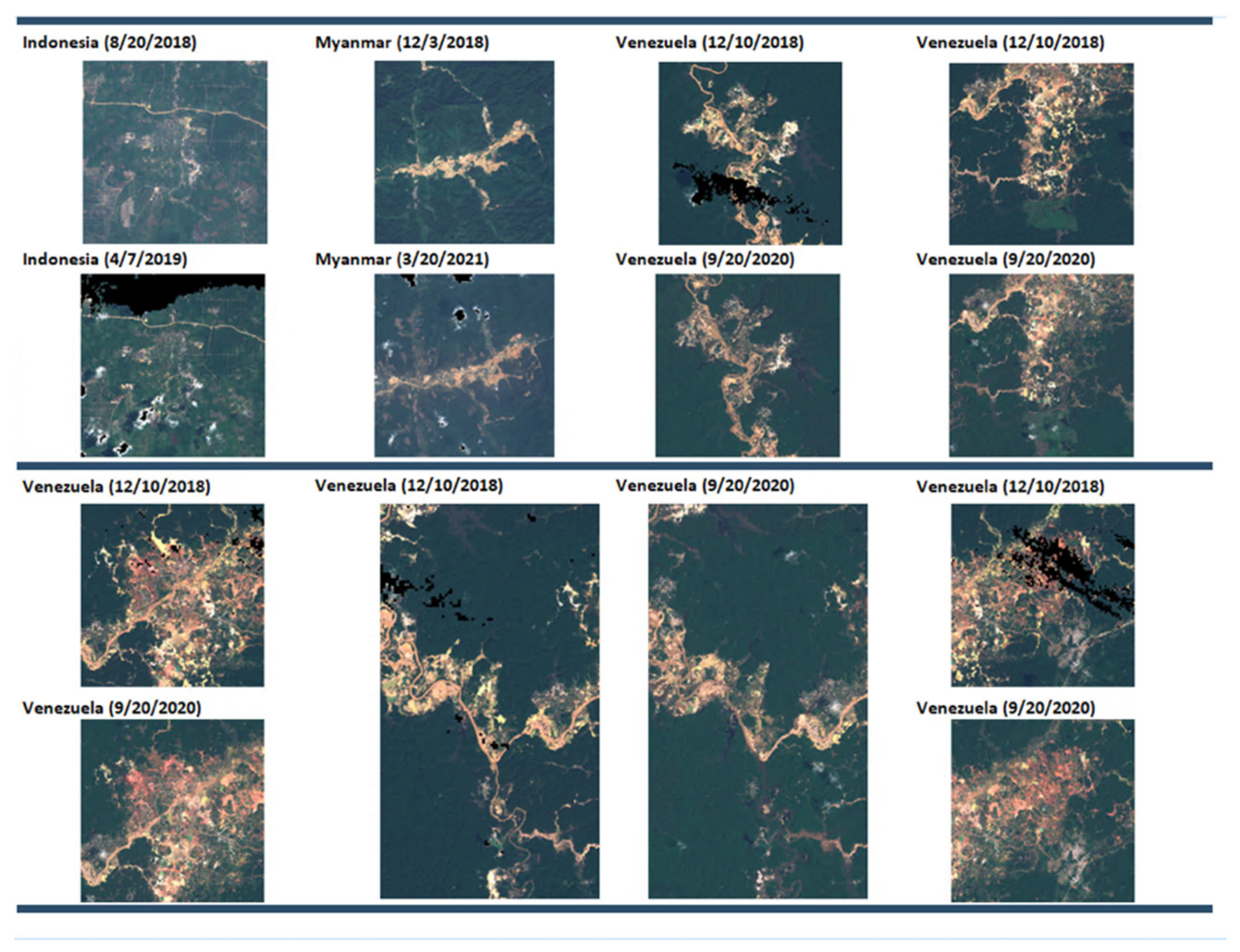
- A test of the best-performing models at a selection of out-of-sample international ASGM sites to examine universal model utility.
2. Materials and Methods
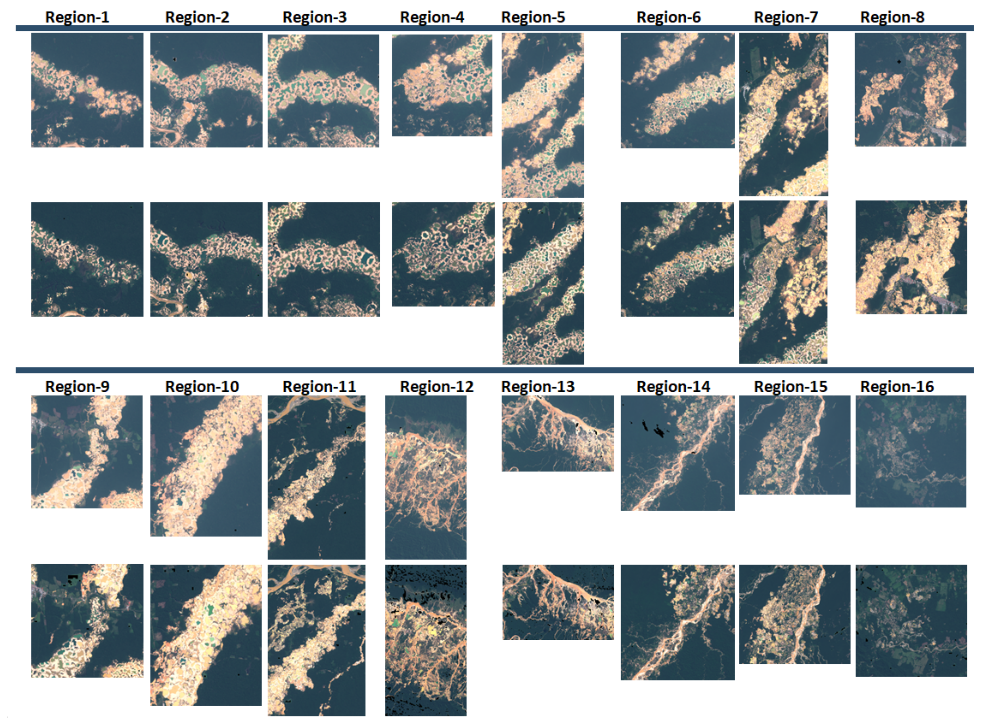
2.1. ASGM Ponds Dataset and Change Characterization
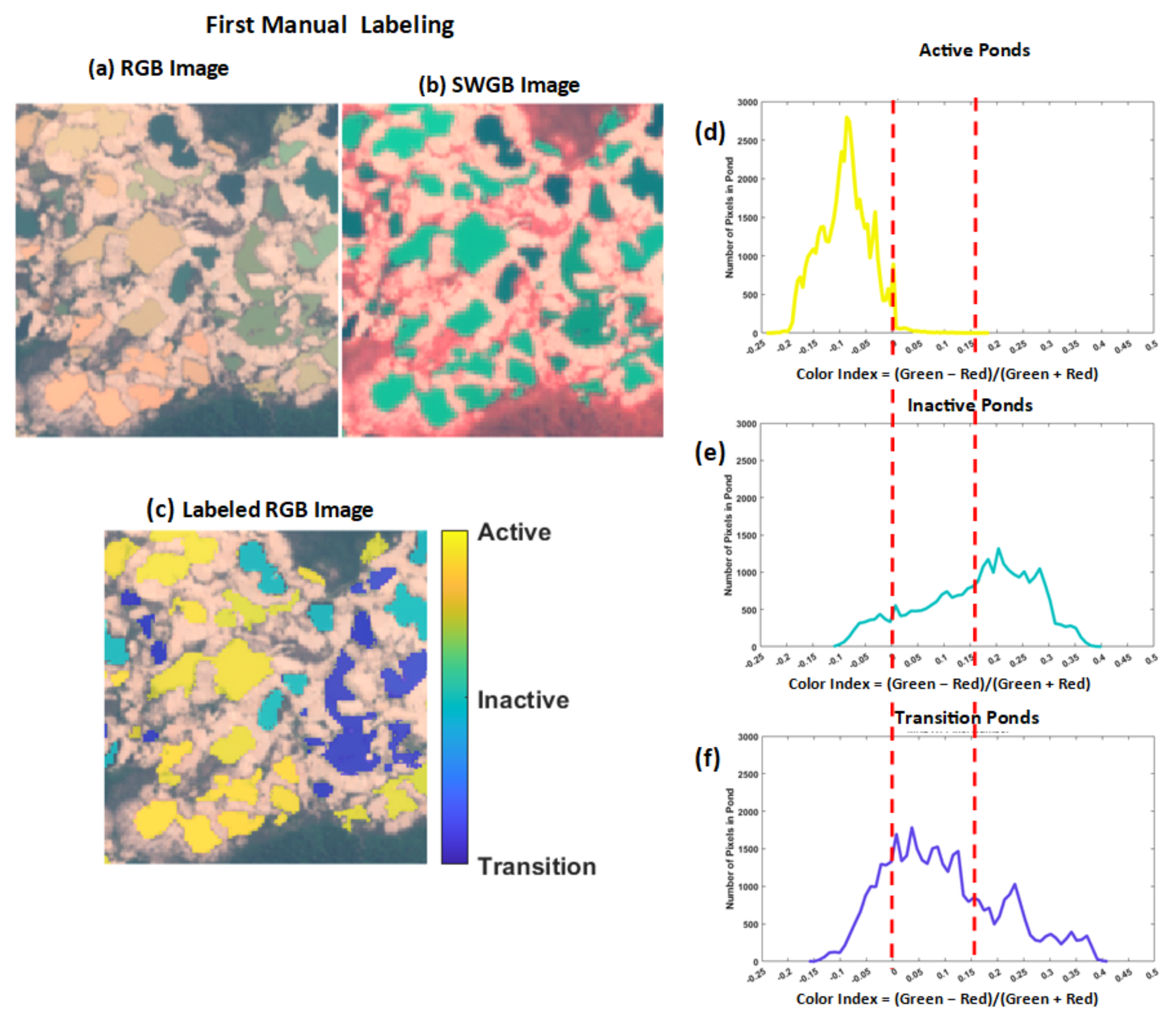
- Active state: where mining was ongoing at the time of image collection;
- Transition state: where mining was recent but not ongoing;
- Inactive state: where mining had ceased longer than 6 months prior to imaging.
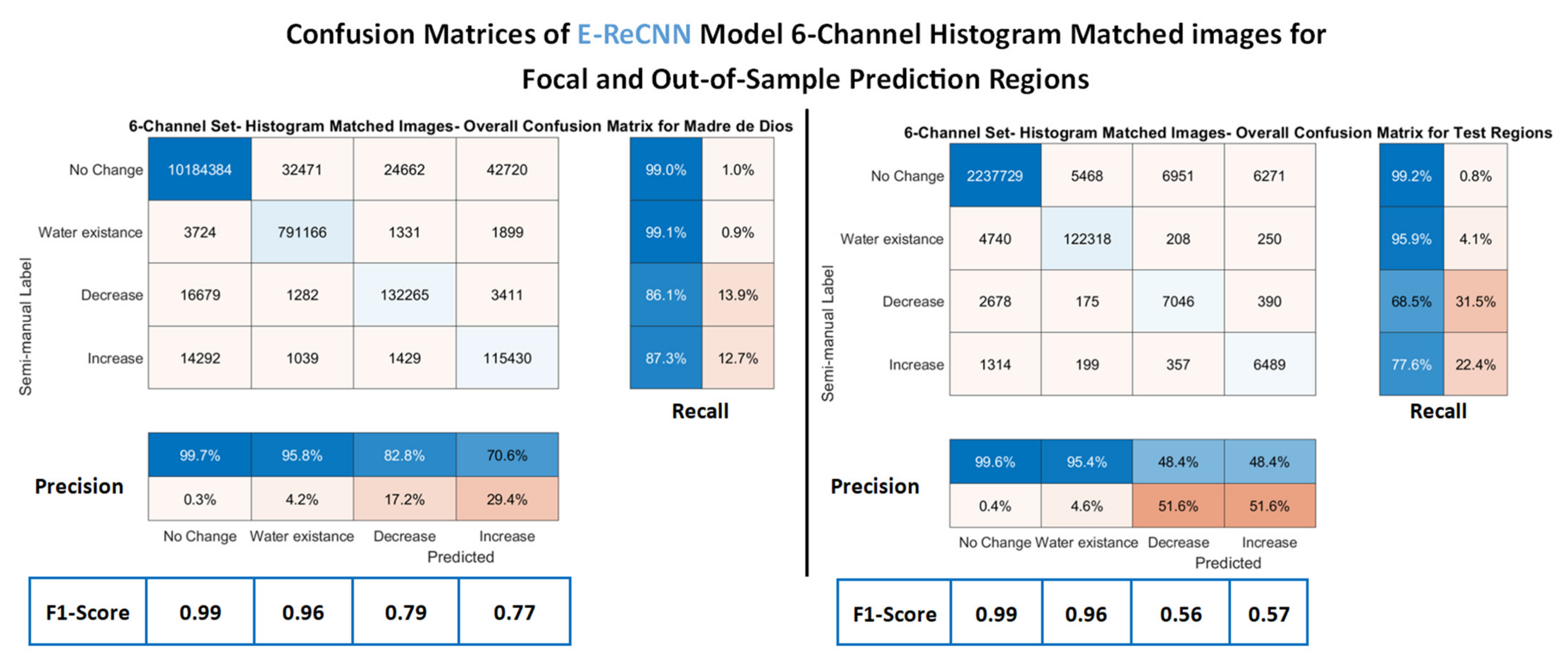
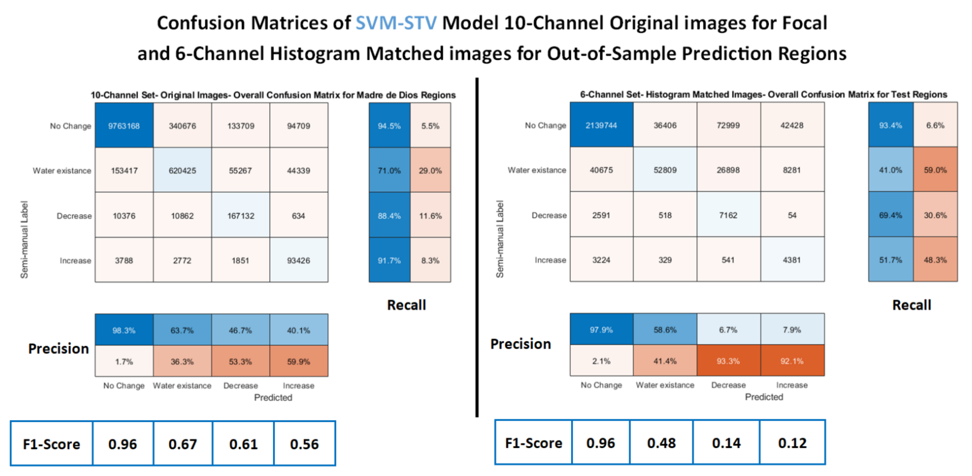
- Decrease: change from active to inactive, active to transition, or transition to inactive;
- Increase: change from inactive to active, inactive to transition, or transition to active;
- Water Existence/Absence: change from water to no-water or no-water to water;
- No Change: no state changes between time periods took place.
2.2. Modeling Approaches
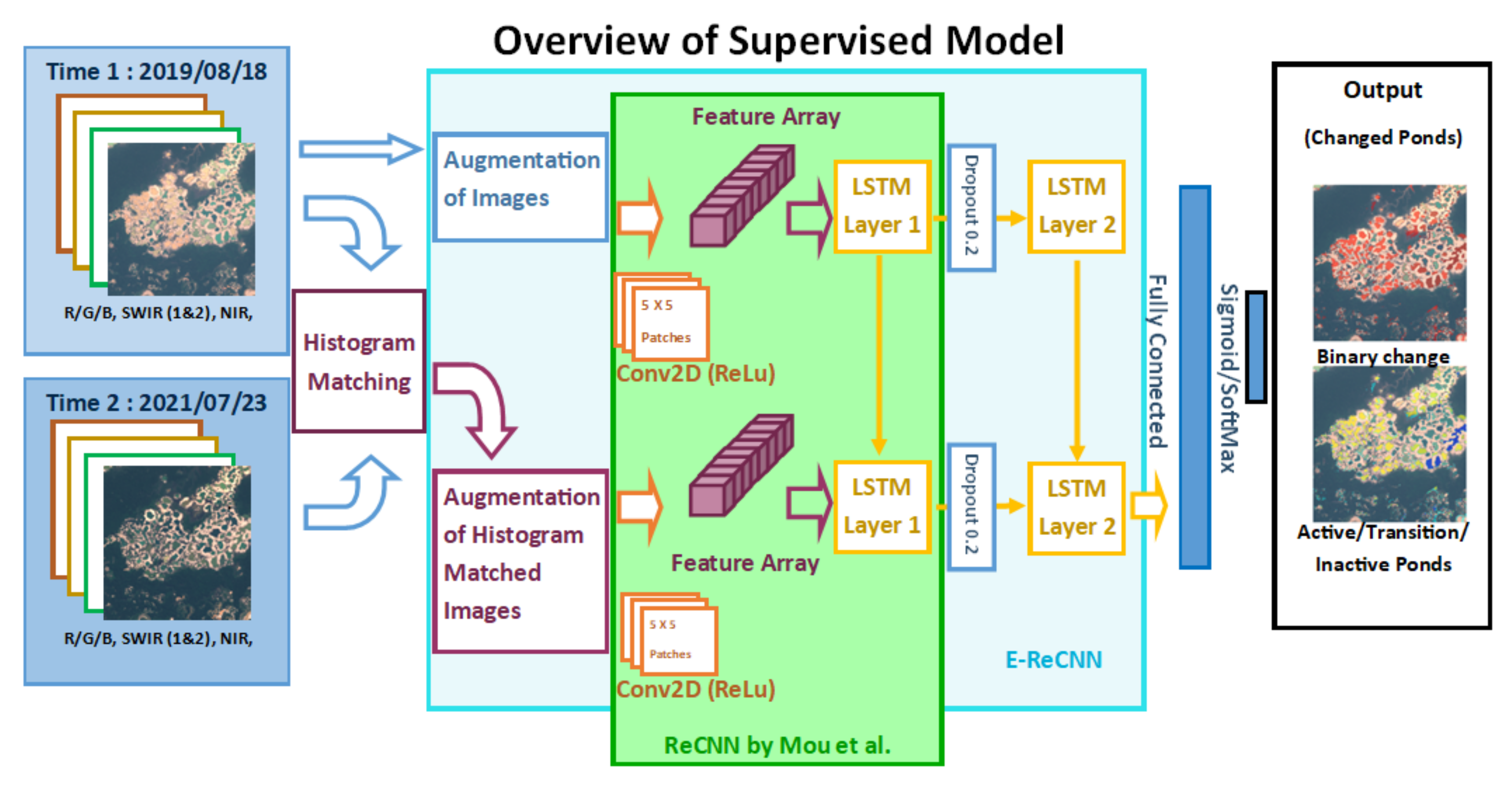
2.2.1. Supervised Deep Learning Approach
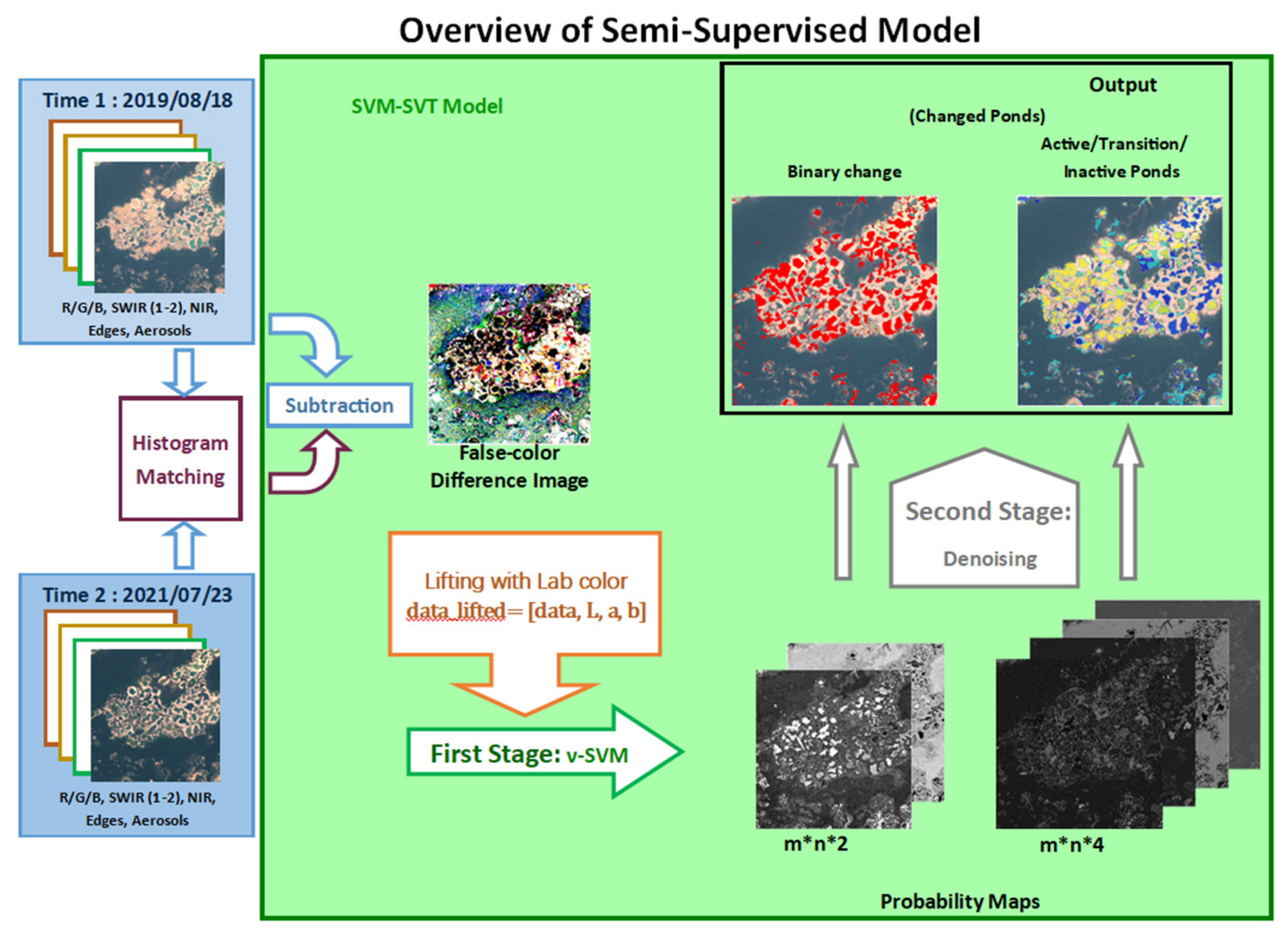
2.2.2. Semi-Supervised Learning Approach
2.2.3. Statistical Approaches, Training, and Operation
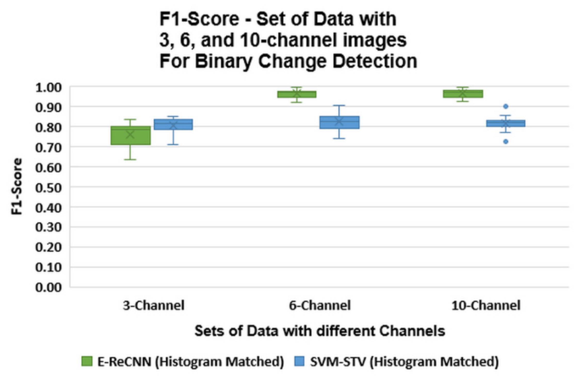
- A three-band set of images containing red, green, and blue bands (RGB);
- A six-band set of images containing red, green, blue, NIR, SWIR1, and SWIR2;
- A 10-band set of images containing red, green, blue, NIR, SWIR-1, SWIR-2, ultra-blue, and bands 5, 6, and 7, which correspond to the vegetation red edge.
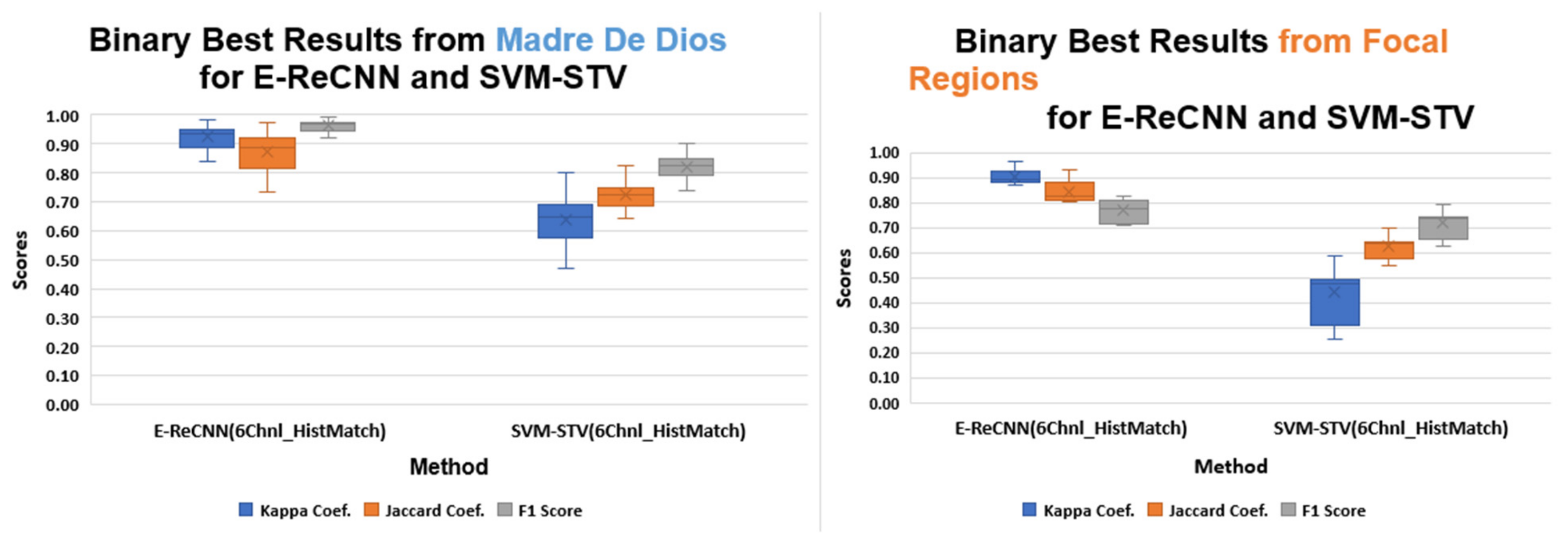
3. Results
4. Discussion
5. Conclusions and Future Work
Author Contributions
Funding
Institutional Review Board Statement
Informed Consent Statement
Data Availability Statement
Acknowledgments
Conflicts of Interest
Appendix A

| Region Number | Size in Pixels | Area in Km2 | Left Bottom | Right Top |
|---|---|---|---|---|
| Region-1 | 667 × 654 | 43.37 | 13°01′51.9″ S 69°55′29.5″ W | 12°58′15.9″ S 69°51′53.5″ W |
| Region-2 | 667 × 655 | 43.37 | 13°01′21.8″ S 69°58′37.3″ W | 12°57′45.8″ S 69°55′01.3″ W |
| Region-3 | 556 × 546 | 30.12 | 13°00′27.3″ S 70°00′54.0″ W | 12°57′27.3″ N 69°57′54.0″ W |
| Region-4 | 556 × 545 | 30.12 | 13°00′43.6″ S 70°03′19.6″ W | 12°57′43.6″ S 70°00′19.6″ W |
| Region-5 | 1109 × 548 | 60.25 | 12°59′42.4″ S 70°02′36.0″ W | 12°53′42.4″ S 69°59′36.0″ W |
| Region-6 | 667 × 655 | 43.38 | 12°59′22.4″ S 70°06′47.8″ W | 12°55′46.4″ S 70°03′11.8″ W |
| Region-7 | 888 × 482 | 42.42 | 12°57′16.3″ S 70°04′57.0″ W | 12°52′28.3″ S 70°02′18.6″ W |
| Region-8 | 556 × 545 | 30.13 | 12°53′31.7″ S 70°03′35.8″ W | 12°50′31.7″ S 70°00′35.8″ W |
| Region-9 | 556 × 546 | 30.13 | 12°55′34.6″ S 70°01′14.7″ W | 12°52′34.6″ S 69°58′14.7″ W |
| Region-10 | 555 × 438 | 24.1 | 12°53′19.3″ S 69°59′47.2″ W | 12°50′19.3″ S 69°57′23.2″ W |
| Region-11 | 1109 × 657 | 86.72 | 12°51′48.2″ S 69°57′52.1″ W | 12°45′48.2″ S 69°54′16.1″ W |
| Region-12 | 1333 × 659 | 86.12 | 13°05′46.4″ S 70°31′00.8″ W | 12°58′34.4″ S 70°27′24.8″ W |
| Region-13 | 894 × 1309 | 115.66 | 13°02′14.2″ S 70°39′33.2″ W | 12°57′26.2″ S 70°32′21.2″ W |
| Region-14 | 1337 × 1311 | 173.56 | 12°56′48.5″ S 70°38′10.1″ W | 12°49′36.5″ S 70°30′58.1″ W |
| Region-15 | 1560 × 1748 | 270.11 | 12°49′54.8″ S 70°35′44.9″ W | 12°41′30.8″ S 70°26′08.9″ W |
| Region-16 | 668 × 655 | 43.38 | 12°57′55.2″ S 70°16′12.7″ W | 12°54′19.2″ S 70°12′36.7″ W |
| E-ReCNN (TensorFlow Framework) | Nesterov Adam − Learning rate − 1 × 10⁻³ Glorot uniform initializer − uniform distribution |
| SVM-STV | The two parameters of ν-SVC: Nu: 0–0.2, Gamma: , where n is the number of bands. The denoising parameters: Alpha1: 0–1, Alpha2: [0, 0.5, 1, 2], Mu: 5. The above five parameters are tuned on each of the 16 training regions. |
| E-ReCNN (Wake Forest University DEAC HPC cluster) | Number of Epochs: 75 | Total Loss: 0.0208 | Time per epoch: 548 s |
| SVM-STV (Local machine) | Number of Trials: 10 | Training Error: Controlled by Nu | Time per trial: 3 s to 94 s |
| Area | Number of Regions | Accuracy | Kappa Coef. | Jaccard Coef. | F1-Score | No Change | Decrease | Increase | Water Existence |
|---|---|---|---|---|---|---|---|---|---|
| La Pampa | 1 | 0.989 | 0.932 | 0.889 | 0.941 | 0.995 | 0.938 | 0.865 | 0.965 |
| 2 | 0.979 | 0.880 | 0.814 | 0.893 | 0.990 | 0.911 | 0.726 | 0.945 | |
| 3 | 0.978 | 0.891 | 0.826 | 0.918 | 0.988 | 0.923 | 0.813 | 0.948 | |
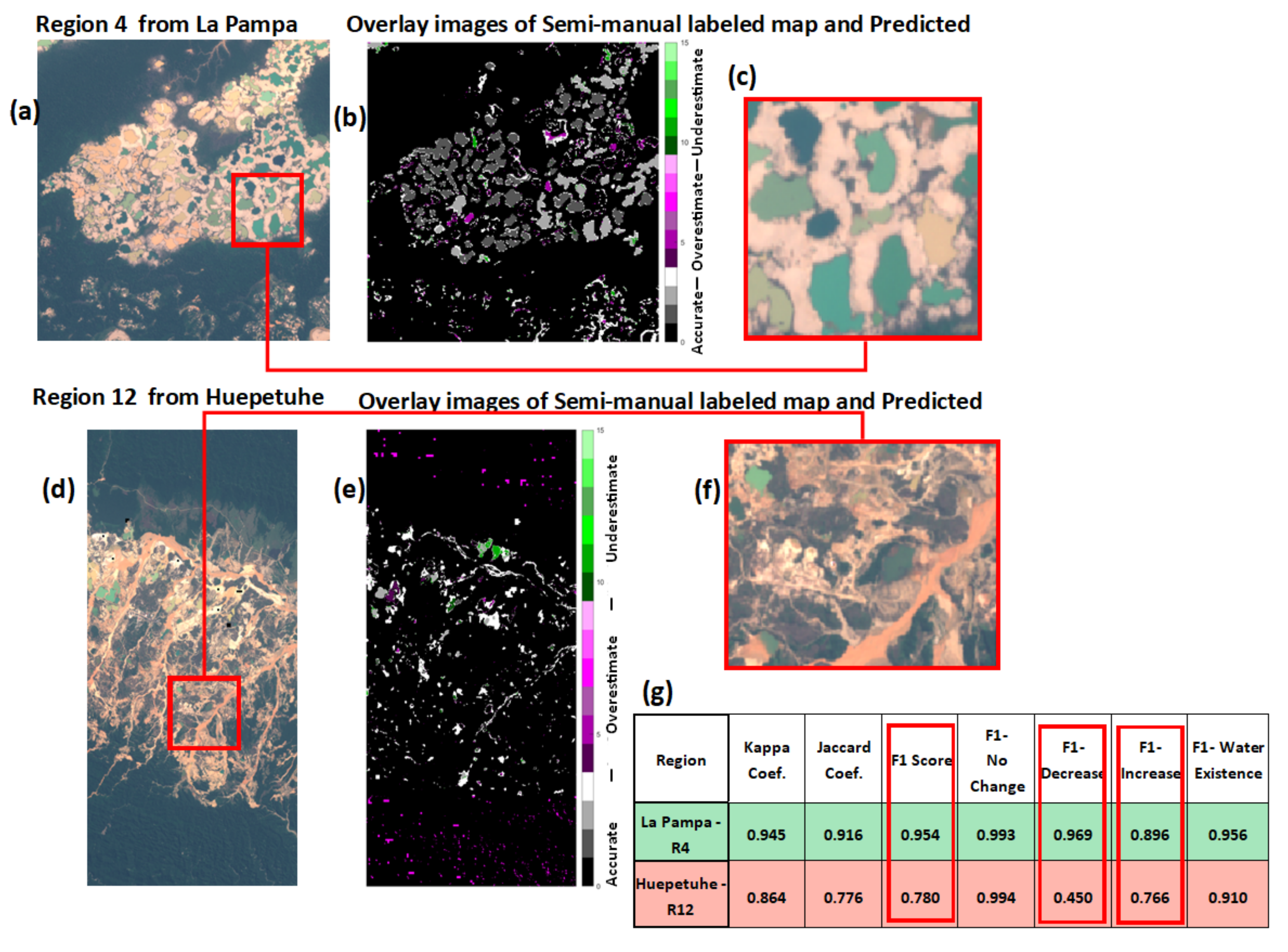
| 4 | 0.986 | 0.945 | 0.916 | 0.954 | 0.993 | 0.969 | 0.896 | 0.956 | |
| 5 | 0.978 | 0.913 | 0.863 | 0.923 | 0.988 | 0.924 | 0.819 | 0.964 | |
| 6 | 0.979 | 0.879 | 0.807 | 0.868 | 0.989 | 0.852 | 0.660 | 0.969 | |
| 7 | 0.987 | 0.951 | 0.921 | 0.887 | 0.993 | 0.884 | 0.685 | 0.985 | |
| 8 | 0.996 | 0.984 | 0.974 | 0.904 | 0.998 | 0.774 | 0.854 | 0.991 | |
| 9 | 0.986 | 0.924 | 0.875 | 0.914 | 0.993 | 0.869 | 0.847 | 0.950 | |
| 10 | 0.995 | 0.983 | 0.973 | 0.930 | 0.997 | 0.805 | 0.927 | 0.990 | |
| 11 | 0.996 | 0.977 | 0.961 | 0.799 | 0.998 | 0.460 | 0.752 | 0.988 | |
| Huepetuhe | 12 | 0.987 | 0.864 | 0.776 | 0.780 | 0.994 | 0.450 | 0.766 | 0.910 |
| 13 | 0.994 | 0.951 | 0.917 | 0.848 | 0.997 | 0.659 | 0.754 | 0.983 | |
| Delta | 14 | 0.989 | 0.924 | 0.884 | 0.855 | 0.995 | 0.686 | 0.772 | 0.970 |
| 15 | 0.985 | 0.930 | 0.889 | 0.839 | 0.992 | 0.636 | 0.740 | 0.987 | |
| Inambari Tributary | 16 | 0.987 | 0.832 | 0.740 | 0.795 | 0.994 | 0.547 | 0.786 | 0.854 |
| Region Number | Time1 | Time2 | Size in Pixels | Area in km2 | Left Bottom | Right Top |
|---|---|---|---|---|---|---|
| Indonesia-1 | 20 August 2018 | 7 April 2019 | 666 × 667 | 44.51 | 0°44′39.4″ N 110°42′25.3″ E | 0°48′15.4″ N 110°46′01.3″ E |
| Myanmar-2 | 3 December 2018 | 20 March 2021 | 664 × 668 | 43.54 | 11°56′19.2″ N 99°16′20.4″ E | 11°59′55.2″ N 99°19′56.4″ E |
| Venezuela-3 | 10 December 2018 | 20 September 2020 | 666 × 667 | 44.25 | 6°11′42.9″ N 61°33′15.9″ W | 6°15′18.9″ N 61°29′39.9″ W |
| Venezuela-4 | 10 December 2018 | 20 September 2020 | 666 × 667 | 44.25 | 6°08′07.3″ N 61°29′46.0″ W | 6°11′43.3″ N 61°26′10.0″ W |
| Venezuela-5 | 10 December 2018 | 20 September 2020 | 556 × 556 | 30.73 | 6°10′19.6″ N 61°29′24.8″ W | 6°13′19.6″ N 61°26′24.8″ W |
| Venezuela-6 | 10 December 2018 | 20 September 2020 | 887 × 490 | 43.27 | 6°08′47.2″ N 61°31′18.5″ W | 6°13′35.2″ N 61°28′40.1″ W |
| Venezuela-7 | 10 December 2018 | 20 September 2020 | 666 × 667 | 44.25 | 6°10′07.4″ N 61°27′48.5″ W | 6°13′43.4″ N 61°24′12.5″ W |
| Kappa Coef. | Jaccard Coef. | F1-Score | |||
|---|---|---|---|---|---|
| Original Images | 3 Channel | Average | 0.63 | 0.52 | 0.81 |
| Std Dev | 0.13 | 0.12 | 0.07 | ||
| 6 Channel | Average | 0.71 | 0.63 | 0.84 | |
| Std Dev | 0.23 | 0.21 | 0.16 | ||
| 10 Channel | Average | 0.70 | 0.62 | 0.83 | |
| Std Dev | 0.25 | 0.23 | 0.17 | ||
| Histogram-Matched Images | 3 Channel | Average | 0.53 | 0.42 | 0.76 |
| Std Dev | 0.11 | 0.11 | 0.06 | ||
| 6 Channel | Average | 0.92 | 0.87 | 0.96 | |
| Std Dev | 0.04 | 0.07 | 0.02 | ||
| 10 Channel | Average | 0.92 | 0.87 | 0.96 | |
| Std Dev | 0.04 | 0.07 | 0.02 | ||
| Histogram-Matched + Lab Lifted Images | 3 Channel | Average | 0.45 | 0.37 | 0.71 |
| Std Dev | 0.16 | 0.14 | 0.10 | ||
| 6 Channel | Average | 0.92 | 0.87 | 0.96 | |
| Std Dev | 0.04 | 0.07 | 0.02 | ||
| 10 Channel | Average | 0.91 | 0.86 | 0.96 | |
| Std Dev | 0.04 | 0.07 | 0.02 |
| Kappa Coef. | Jaccard Coef. | F1-Score | |||
|---|---|---|---|---|---|
| Original Images | 3 Channel | Average | 0.44 | 0.60 | 0.72 |
| Std Dev | 0.10 | 0.06 | 0.06 | ||
| 6 Channel | Average | 0.62 | 0.71 | 0.81 | |
| Std Dev | 0.08 | 0.05 | 0.04 | ||
| 10 Channel | Average | 0.67 | 0.74 | 0.84 | |
| Std Dev | 0.07 | 0.04 | 0.03 | ||
| Histogram-Matched Images | 3 Channel | Average | 0.52 | 0.65 | 0.76 |
| Std Dev | 0.09 | 0.06 | 0.05 | ||
| 6 Channel | Average | 0.64 | 0.72 | 0.82 | |
| Std Dev | 0.07 | 0.04 | 0.03 | ||
| 10 Channel | Average | 0.62 | 0.71 | 0.81 | |
| Std Dev | 0.09 | 0.05 | 0.05 | ||
| Histogram-Matched + Lab-Lifted Images | 3 Channel | Average | 0.61 | 0.71 | 0.80 |
| Std Dev | 0.07 | 0.04 | 0.04 | ||
| 6 Channel | Average | 0.64 | 0.72 | 0.82 | |
| Std Dev | 0.08 | 0.04 | 0.04 | ||
| 10 Channel | Average | 0.62 | 0.71 | 0.81 | |
| Std Dev | 0.08 | 0.04 | 0.04 |
Appendix B


References
- Dethier, E.N.; Sartain, S.L.; Lutz, D.A. Heightened Levels and Seasonal Inversion of Riverine Suspended Sediment in a Tropical Biodiversity Hot Spot Due to Artisanal Gold Mining. Proc. Natl. Acad. Sci. USA 2019, 116, 23936–23941. [Google Scholar] [CrossRef] [PubMed]
- Alvarez-Berrios, N.L.; Mitchell Aide, T. Global Demand for Gold Is Another Threat for Tropical Forests. Environ. Res. Lett. 2015, 10, 14006. [Google Scholar] [CrossRef] [Green Version]
- Kahhat, R.; Parodi, E.; Larrea-Gallegos, G.; Mesta, C.; Vázquez-Rowe, I. Environmental Impacts of the Life Cycle of Alluvial Gold Mining in the Peruvian Amazon Rainforest. Sci. Total Environ. 2019, 662, 940–951. [Google Scholar] [CrossRef] [PubMed]
- Caballero Espejo, J.; Messinger, M.; Román-Dañobeytia, F.; Ascorra, C.; Fernandez, L.E.; Silman, M. Deforestation and Forest Degradation Due to Gold Mining in the Peruvian Amazon: A 34-Year Perspective. Remote Sens. 2018, 10, 1903. [Google Scholar] [CrossRef] [Green Version]
- Taiwo, A.M.; Awomeso, J.A. Assessment of Trace Metal Concentration and Health Risk of Artisanal Gold Mining Activities in Ijeshaland, Osun State Nigeria–Part 1. J. Geochem. Explor. 2017, 177, 1–10. [Google Scholar] [CrossRef]
- Owusu-Nimo, F.; Mantey, J.; Nyarko, K.B.; Appiah-Effah, E.; Aubynn, A. Spatial Distribution Patterns of Illegal Artisanal Small Scale Gold Mining (Galamsey) Operations in Ghana: A Focus on the Western Region. Heliyon 2018, 4, e00534. [Google Scholar] [CrossRef] [PubMed] [Green Version]
- Bounliyong, P.; Itaya, T.; Arribas, A.; Watanabe, Y.; Wong, H.; Echigo, T. K–Ar Geochronology of Orogenic Gold Mineralization in the Vangtat Gold Belt, Southeastern Laos: Effect of Excess Argon in Hydrothermal Quartz. Resour. Geol. 2021, 71, 161–175. [Google Scholar] [CrossRef]
- Kimijima, S.; Sakakibara, M.; Nagai, M. Detection of Artisanal and Small-Scale Gold Mining Activities and Their Transformation Using Earth Observation, Nighttime Light, and Precipitation Data. Int. J. Environ. Res. Public Health 2021, 18, 10954. [Google Scholar] [CrossRef]
- Gonzalez, D.J.X.; Arain, A.; Fernandez, L.E. Mercury Exposure, Risk Factors, and Perceptions among Women of Childbearing Age in an Artisanal Gold Mining Region of the Peruvian Amazon. Environ. Res. 2019, 179, 108786. [Google Scholar] [CrossRef] [PubMed]
- Gerson, J.R.; Topp, S.N.; Vega, C.M.; Gardner, J.R.; Yang, X.; Fernandez, L.E.; Bernhardt, E.S.; Pavelsky, T.M. Artificial Lake Expansion Amplifies Mercury Pollution from Gold Mining. Sci. Adv. 2020, 6, eabd4953. [Google Scholar] [CrossRef] [PubMed]
- Swenson, J.J.; Carter, C.E.; Domec, J.-C.; Delgado, C.I. Gold Mining in the Peruvian Amazon: Global Prices, Deforestation, and Mercury Imports. PLoS ONE 2011, 6, e18875. [Google Scholar] [CrossRef] [PubMed] [Green Version]
- Cooley, S.; Smith, L.; Stepan, L.; Mascaro, J. Tracking Dynamic Northern Surface Water Changes with High-Frequency Planet CubeSat Imagery. Remote Sens. 2017, 9, 1306. [Google Scholar] [CrossRef] [Green Version]
- Zou, Z.; Dong, J.; Menarguez, M.A.; Xiao, X.; Qin, Y.; Doughty, R.B.; Hooker, K.V.; David Hambright, K. Continued Decrease of Open Surface Water Body Area in Oklahoma during 1984–2015. Sci. Total Environ. 2017, 595, 451–460. [Google Scholar] [CrossRef] [PubMed]
- Wang, C.; Jia, M.; Chen, N.; Wang, W. Long-Term Surface Water Dynamics Analysis Based on Landsat Imagery and the Google Earth Engine Platform: A Case Study in the Middle Yangtze River Basin. Remote Sens. 2018, 10, 1635. [Google Scholar] [CrossRef] [Green Version]
- Kruger, N.; Janssen, P.; Kalkan, S.; Lappe, M.; Leonardis, A.; Piater, J.; Rodriguez-Sanchez, A.J.; Wiskott, L. Deep Hierarchies in the Primate Visual Cortex: What Can We Learn for Computer Vision? IEEE Trans. Pattern Anal. Mach. Intell. 2013, 35, 1847–1871. [Google Scholar] [CrossRef]
- Camalan, S.; Niazi, M.K.K.; Moberly, A.C.; Teknos, T.; Essig, G.; Elmaraghy, C.; Taj-Schaal, N.; Gurcan, M.N. OtoMatch: Content-Based Eardrum Image Retrieval Using Deep Learning. PLoS ONE 2020, 15, e0232776. [Google Scholar] [CrossRef] [PubMed]
- Morchhale, S.; Pauca, V.P.; Plemmons, R.J.; Torgersen, T.C. Classification of Pixel-Level Fused Hyperspectral and Lidar Data Using Deep Convolutional Neural Networks. In Proceedings of the 2016 8th Workshop on Hyperspectral Image and Signal Processing: Evolution in Remote Sensing (WHISPERS), Los Angeles, CA, USA, 21–24 August 2016; pp. 1–5. [Google Scholar] [CrossRef]
- Camalan, S.; Mahmood, H.; Binol, H.; Araújo, A.L.D.; Santos-Silva, A.R.; Vargas, P.A.; Lopes, M.A.; Ali, K.S.; Gurcan, M.N. Convolutional Neural Network-Based Clinical Predictors of Oral Dysplasia: Class Activation Map Analysis of Deep Learning Results. Cancers 2021, 13, 1291. [Google Scholar] [CrossRef] [PubMed]
- Yuan, X.; Shi, J.; Gu, L. A Review of Deep Learning Methods for Semantic Segmentation of Remote Sensing Imagery. Expert Syst. Appl. 2021, 169, 114417. [Google Scholar] [CrossRef]
- Mohan, A.; Singh, A.K.; Kumar, B.; Dwivedi, R. Review on Remote Sensing Methods for Landslide Detection Using Machine and Deep Learning. Trans. Emerg. Telecommun. Technol. 2021, 32, e3998. [Google Scholar] [CrossRef]
- Hoeser, T.; Kuenzer, C. Object Detection and Image Segmentation with Deep Learning on Earth Observation Data: A Review-Part I: Evolution and Recent Trends. Remote Sens. 2020, 12, 1667. [Google Scholar] [CrossRef]
- Hoeser, T.; Bachofer, F.; Kuenzer, C. Object Detection and Image Segmentation with Deep Learning on Earth Observation Data: A Review—Part II: Applications. Remote Sens. 2020, 12, 3053. [Google Scholar] [CrossRef]
- Khelifi, L.; Mignotte, M. Deep Learning for Change Detection in Remote Sensing Images: Comprehensive Review and Meta-Analysis. IEEE Access 2020, 8, 126385–126400. [Google Scholar] [CrossRef]
- Lyu, H.; Lu, H.; Mou, L. Learning a Transferable Change Rule from a Recurrent Neural Network for Land Cover Change Detection. Remote Sens. 2016, 8, 506. [Google Scholar] [CrossRef] [Green Version]
- Ienco, D.; Gaetano, R.; Dupaquier, C.; Maurel, P. Land Cover Classification via Multitemporal Spatial Data by Deep Recurrent Neural Networks. IEEE Geosci. Remote Sens. Lett. 2017, 14, 1685–1689. [Google Scholar] [CrossRef] [Green Version]
- Rußwurm, M.; Körner, M. Temporal Vegetation Modelling Using Long Short-Term Memory Networks for Crop Identification from Medium-Resolution Multi-Spectral Satellite Images. In Proceedings of the IEEE Conference on Computer Vision and Pattern Recognition Workshops, Venice, Italy, 22–29 October 2017; pp. 11–19. [Google Scholar]
- Zhong, L.; Hu, L.; Zhou, H. Deep Learning Based Multi-Temporal Crop Classification. Remote Sens. Environ. 2019, 221, 430–443. [Google Scholar] [CrossRef]
- Mou, L.; Bruzzone, L.; Zhu, X.X. Learning Spectral-Spatial-Temporal Features via a Recurrent Convolutional Neural Network for Change Detection in Multispectral Imagery. IEEE Trans. Geosci. Remote Sens. 2019, 57, 924–935. [Google Scholar] [CrossRef] [Green Version]
- Asner, G.P.; Tupayachi, R. Accelerated Losses of Protected Forests from Gold Mining in the Peruvian Amazon. Environ. Res. Lett. 2016, 12, 094004. [Google Scholar] [CrossRef]
- Dethier, E.N.; Silman, M.; Fernandez, L.E.; Espejo, J.C.; Alqahtani, S.; Pauca, P.V.; Lutz, D.A. Operation Mercury: Impacts of National-Level Military-Based Enforcement Strategy and COVID-19 on Artisanal Gold Mining and Water Quality in a Biodiversity Hotspot in the Peruvian Amazon. (under review to the Conservation Letter journal and revision submitted on 26 January 2022).
- Drusch, M.; del Bello, U.; Carlier, S.; Colin, O.; Fernandez, V.; Gascon, F.; Hoersch, B.; Isola, C.; Laberinti, P.; Martimort, P.; et al. Sentinel-2: ESA’s Optical High-Resolution Mission for GMES Operational Services. Remote Sens. Environ. 2012, 120, 25–36. [Google Scholar] [CrossRef]
- Cordeiro, M.C.R.; Martinez, J.M.; Peña-Luque, S. Automatic Water Detection from Multidimensional Hierarchical Clustering for Sentinel-2 Images and a Comparison with Level 2A Processors. Remote Sens. Environ. 2021, 253, 112209. [Google Scholar] [CrossRef]
- Pahlevan, N.; Smith, B.; Schalles, J.; Binding, C.; Cao, Z.; Ma, R.; Alikas, K.; Kangro, K.; Gurlin, D.; Hà, N.; et al. Seamless Retrievals of Chlorophyll-a from Sentinel-2 (MSI) and Sentinel-3 (OLCI) in Inland and Coastal Waters: A Machine-Learning Approach. Remote Sens. Environ. 2020, 240, 111604. [Google Scholar] [CrossRef]
- Chan, R.H.; Kan, K.K.; Nikolova, M.; Plemmons, R.J. A Two-Stage Method for Spectral–Spatial Classification of Hyperspectral Images. J. Math. Imaging Vis. 2020, 62, 790–807. [Google Scholar] [CrossRef] [Green Version]
- Peng, D.; Zhang, Y.; Guan, H. End-to-End Change Detection for High Resolution Satellite Images Using Improved UNet++. Remote Sens. 2019, 11, 1382. [Google Scholar] [CrossRef] [Green Version]
- Chen, L.; Zhang, D.; Li, P.; Lv, P. Change Detection of Remote Sensing Images Based on Attention Mechanism. Comput. Intell. Neurosci. 2020, 2020, 6430627. [Google Scholar] [CrossRef]
- Melgani, F.; Bruzzone, L. Classification of Hyperspectral Remote Sensing Images with Support Vector Machines. IEEE Trans. Geosci. Remote Sens. 2004, 42, 1778–1790. [Google Scholar] [CrossRef] [Green Version]
- Camps-Valls, G.; Bruzzone, L. Kernel-Based Methods for Hyperspectral Image Classification. IEEE Trans. Geosci. Remote Sens. 2005, 43, 1351–1362. [Google Scholar] [CrossRef]
- Camps-Valls, G.; Gomez-Chova, L.; Muñoz-Marí, J.; Vila-Francés, J.; Calpe-Maravilla, J. Composite Kernels for Hyperspectral Image Classification. IEEE Geosci. Remote Sens. Lett. 2006, 3, 93–97. [Google Scholar] [CrossRef]
- Rotaru, C.; Graf, T.; Zhang, J. Color Image Segmentation in HSI Space for Automotive Applications. J. Real-Time Image Processing 2008, 3, 311–322. [Google Scholar] [CrossRef]
- Paschos, G. Perceptually Uniform Color Spaces for Color Texture Analysis: An Empirical Evaluation. IEEE Trans. Image Process. 2001, 10, 932–937. [Google Scholar] [CrossRef] [Green Version]
- Cardelino, J.; Caselles, V.; Bertalmío, M.; Randall, G. A Contrario Selection of Optimal Partitions for Image Segmentation. SIAM J. Imaging Sci. 2013, 6, 1274–1317. [Google Scholar] [CrossRef] [Green Version]
- Cai, X.; Chan, R.; Nikolova, M.; Zeng, T. A Three-Stage Approach for Segmenting Degraded Color Images: Smoothing, Lifting and Thresholding (SLaT). J. Sci. Comput. 2017, 72, 1313–1332. [Google Scholar] [CrossRef] [Green Version]
- Schölkopf, B.; Smola, A.J.; Williamson, R.C.; Bartlett, P.L. New Support Vector Algorithms. Neural Comput. 2000, 12, 1207–1245. [Google Scholar] [CrossRef] [PubMed]
- Hsu, C.W.; Lin, C.J. A Comparison of Methods for Multiclass Support Vector Machines. IEEE Trans. Neural Netw. 2002, 13, 415–425. [Google Scholar] [CrossRef] [PubMed] [Green Version]
- Binol, H.; Plotner, A.; Sopkovich, J.; Kaffenberger, B.; Niazi, M.K.K.; Gurcan, M.N. Ros-NET: A Deep Convolutional Neural Network for Automatic Identification of Rosacea Lesions. Skin Res. Technol. 2020, 26, 413–421. [Google Scholar] [CrossRef] [PubMed]
- Dozat, T. Workshop Track-ICLR 2016 INCORPORATING NESTEROV MOMENTUM INTO ADAM. In Proceedings of the International Conference on Learning Representations Workshop, San Juan, Puerto Rico, 2–4 May 2016. [Google Scholar]
- Tato, A.; Nkambou, R. Improving ADAM Optimizer. In Proceedings of the Workshop Track-ICLR 2018, Vancouver, BC, Canada, 30 April–3 May 2018. [Google Scholar]
- Information Systems and Wake Forest University. WFU High Performance Computing Facility. Available online: https://is.wfu.edu/services/high-performance-computing/ (accessed on 27 February 2022). [CrossRef]
- Cohen, J. A Coefficient of Agreement for Nominal Scales. Educ. Psychol. Meas. 1960, 20, 37–46. [Google Scholar] [CrossRef]
- Jaccard, P. Distribution de La Flore Alpine Dans Le Bassin Des Dranses et Dans Quelques Regions Voisines. Bull. De La Société Vaud. Des Sci. Nat. 1901, 37, 241–272. [Google Scholar]
- Dice, L.R. Measures of the Amount of Ecologic Association Between Species. Ecology 1945, 26, 297–302. [Google Scholar] [CrossRef]
- Sørensen, T. A Method of Establishing Groups of Equal Amplitude in Plant Sociology Based on Similarity. K. Dan. Vidensk. Selsk. Biol. Skr. 1948, 5, 1–34. [Google Scholar]
- Lyapustin, A.I.; Wang, Y.; Laszlo, I.; Hilker, T.; Hall, F.G.; Sellers, P.J.; Tucker, C.J.; Korkin, S.V. Multi-Angle Implementation of Atmospheric Correction for MODIS (MAIAC): 3. Atmospheric Correction. Remote Sens. Environ. 2012, 127, 385–393. [Google Scholar] [CrossRef]
- Claverie, M.; Ju, J.; Masek, J.G.; Dungan, J.L.; Vermote, E.F.; Roger, J.C.; Skakun, S.V.; Justice, C. The Harmonized Landsat and Sentinel-2 Surface Reflectance Data Set. Remote Sens. Environ. 2018, 219, 145–161. [Google Scholar] [CrossRef]
- Vermote, E.; Justice, C.; Claverie, M.; Franch, B. Preliminary Analysis of the Performance of the Landsat 8/OLI Land Surface Reflectance Product. Remote Sens. Environ. 2016, 185, 46–56. [Google Scholar] [CrossRef]
- Masek, J.G.; Vermote, E.F.; Saleous, N.E.; Wolfe, R.; Hall, F.G.; Huemmrich, K.F.; Gao, F.; Kutler, J.; Lim, T.K. A Landsat Surface Reflectance Dataset for North America, 1990–2000. IEEE Geosci. Remote Sens. Lett. 2006, 3, 68–72. [Google Scholar] [CrossRef]
- Tai, Y.W.; Jia, J.; Tang, C.K. Local Color Transfer via Probabilistic Segmentation by Expectation-Maximization. In Proceedings of the 2005 IEEE Computer Society Conference on Computer Vision and Pattern Recognition, CVPR 2005, San Diego, CA, USA, 20–26 June 2005; Volume I. [Google Scholar] [CrossRef] [Green Version]
- Bruzzone, L.; Prieto, D.F.; Serpico, S.B. A Neural-Statistical Approach to Multitemporal and Multisource Remote-Sensing Image Classification. IEEE Trans. Geosci. Remote Sens. 1999, 37, 1350–1359. [Google Scholar] [CrossRef] [Green Version]
- Wiratama, W.; Lee, J.; Sim, D. Change Detection on Multi-Spectral Images Based on Feature-Level U-Net. IEEE Access 2020, 8, 12279–12289. [Google Scholar] [CrossRef]
- Chen, H.; Wu, C.; Du, B.; Zhang, L.; Wang, L. Change Detection in Multisource VHR Images via Deep Siamese Convolutional Multiple-Layers Recurrent Neural Network. IEEE Trans. Geosci. Remote Sens. 2020, 58, 2848–2864. [Google Scholar] [CrossRef]
- Kartal, H.; Alganci, U.; Sertel, E. Histogram Matching Based Mosaicking of SPOT 6/7 Satellite Images. In Proceedings of the 9th International Conference on Recent Advances in Space Technologies, RAST 2019, Istanbul, Turkey, 10–14 June 2019. [Google Scholar] [CrossRef]
- Wieland, M.; Martinis, S. Large-Scale Surface Water Change Observed by Sentinel-2 during the 2018 Drought in Germany. Int. J. Remote Sens. 2020, 41, 4742–4756. [Google Scholar] [CrossRef]
- Zeng, Y.; Yang, X.; Fang, N.; Shi, Z. Large-Scale Afforestation Significantly Increases Permanent Surface Water in China’s Vegetation Restoration Regions. Agric. For. Meteorol. 2020, 290, 108001. [Google Scholar] [CrossRef]
- Ji, L.; Gong, P.; Wang, J.; Shi, J.; Zhu, Z. Construction of the 500-m Resolution Daily Global Surface Water Change Database (2001–2016). Water Resour. Res. 2018, 54, 10–270. [Google Scholar] [CrossRef]
- Shao, P.; Shi, W.; He, P.; Hao, M.; Zhang, X. Novel Approach to Unsupervised Change Detection Based on a Robust Semi-Supervised FCM Clustering Algorithm. Remote Sens. 2016, 8, 264. [Google Scholar] [CrossRef] [Green Version]
- Liu, S.; Marinelli, D.; Bruzzone, L.; Bovolo, F. A Review of Change Detection in Multitemporal Hyperspectral Images: Current Techniques, Applications, and Challenges. IEEE Geosci. Remote Sens. Mag. 2019, 7, 140–158. [Google Scholar] [CrossRef]
- Liu, S.; Du, Q.; Tong, X.; Samat, A.; Bruzzone, L.; Bovolo, F. Multiscale Morphological Compressed Change Vector Analysis for Unsupervised Multiple Change Detection. IEEE J. Sel. Top. Appl. Earth Obs. Remote Sens. 2017, 10, 4124–4137. [Google Scholar] [CrossRef]
- Maggioni, M.; Murphy, J.M. Learning by Unsupervised Nonlinear Diffusion. J. Mach. Learn. Res. 2019, 20, 1–56. [Google Scholar]
- Murphy, J.M.; Maggioni, M. Unsupervised Clustering and Active Learning of Hyperspectral Images with Nonlinear Diffusion. IEEE Trans. Geosci. Remote Sens. 2019, 57, 1829–1845. [Google Scholar] [CrossRef] [Green Version]
- Polk, S.L.; Murphy, J.M. Multiscale Clustering of Hyperspectral Images Through Spectral-Spatial Diffusion Geometry. In Proceedings of the 2021 IEEE International Geoscience and Remote Sensing Symposium IGARSS, Brussels, Belgium, 11–16 July 2021; pp. 4688–4691. [Google Scholar] [CrossRef]


Publisher’s Note: MDPI stays neutral with regard to jurisdictional claims in published maps and institutional affiliations. |
© 2022 by the authors. Licensee MDPI, Basel, Switzerland. This article is an open access article distributed under the terms and conditions of the Creative Commons Attribution (CC BY) license (https://creativecommons.org/licenses/by/4.0/).
Share and Cite
Camalan, S.; Cui, K.; Pauca, V.P.; Alqahtani, S.; Silman, M.; Chan, R.; Plemmons, R.J.; Dethier, E.N.; Fernandez, L.E.; Lutz, D.A. Change Detection of Amazonian Alluvial Gold Mining Using Deep Learning and Sentinel-2 Imagery. Remote Sens. 2022, 14, 1746. https://doi.org/10.3390/rs14071746
Camalan S, Cui K, Pauca VP, Alqahtani S, Silman M, Chan R, Plemmons RJ, Dethier EN, Fernandez LE, Lutz DA. Change Detection of Amazonian Alluvial Gold Mining Using Deep Learning and Sentinel-2 Imagery. Remote Sensing. 2022; 14(7):1746. https://doi.org/10.3390/rs14071746
Chicago/Turabian StyleCamalan, Seda, Kangning Cui, Victor Paul Pauca, Sarra Alqahtani, Miles Silman, Raymond Chan, Robert Jame Plemmons, Evan Nylen Dethier, Luis E. Fernandez, and David A. Lutz. 2022. "Change Detection of Amazonian Alluvial Gold Mining Using Deep Learning and Sentinel-2 Imagery" Remote Sensing 14, no. 7: 1746. https://doi.org/10.3390/rs14071746
APA StyleCamalan, S., Cui, K., Pauca, V. P., Alqahtani, S., Silman, M., Chan, R., Plemmons, R. J., Dethier, E. N., Fernandez, L. E., & Lutz, D. A. (2022). Change Detection of Amazonian Alluvial Gold Mining Using Deep Learning and Sentinel-2 Imagery. Remote Sensing, 14(7), 1746. https://doi.org/10.3390/rs14071746