Diagnostics of Coherent Eddy Transport in the South China Sea Based on Satellite Observations

Abstract

The large discrepancy between Eulerian and Lagrangian work motivates us to examine the leakage of Eulerian eddies and quantify the contribution of coherent eddy transport in the South China Sea (SCS). In this study, Lagrangian particles with a resolution of 1/32° are advected by surface geostrophic currents derived from satellite observations spanning 23 years, and two types of methods are employed to identify sea surface height (SSH) eddies and Lagrangian coherent structures. SSH eddies are proven to be highly leaky during their lifetimes, with more than 80% of the original water leaking out of the eddy interior. As a result of zonal and meridional eddy propagation, the leaked water exhibits a spatial pattern of asymmetry relative to the eddy center. The degree of eddy leakage is found to be independent of several eddy parameters including the nonlinearity parameter U/c, which has been commonly used to assess eddy coherency. Finally, the Lagrangian coherent structures in the SCS are diagnosed and the associated coherent eddy diffusivity is calculated. It is found that coherent eddies contribute to less than 5% of the total eddy material transport in both zonal and meridional directions. These findings suggest that previous studies based on the Eulerian framework significantly overestimate the contribution of coherent eddy transport in the SCS.

1. Introduction

As rotating structures with horizontal scales of ~100 km, mesoscale eddies are ubiquitous in the global oceans. They often last several weeks to months, storing a significant proportion of the ocean’s kinetic energy [1,2,3]. These eddies trap, transport, and stir oceanic tracers such as heat, salt, and nutrients, thus having crucial impacts on ocean circulations, biochemical processes, and the global climate system [4,5,6].

As the largest semi-closed marginal sea in the northwest Pacific, the South China Sea (SCS) has an active current system with multiscale processes that are primarily attributed to the seasonally reversing monsoon, complex bottom topography, and Kuroshio intrusion [7,8]. These dynamical conditions facilitate the generation of instabilities, which transform the SCS into a “zoo” of mesoscale eddies. Previous investigations have reported statistical features of eddy properties [9,10] and estimates of eddy material transport [11,12] in the SCS using both observations and numerical simulations. However, the strength of coherent eddy transport remains unclear due to different eddy definitions used in previous studies, which motivates us to revisit this issue.

The coherent structure is characterized by that the interior water mass is enclosed by a material barrier (boundary) and transported for a distance without volume exchange with the ambient flows [13]. Because of their ability to trap and transport materials, mesoscale eddies are typically treated as coherent structures when the nonlinearity parameter U/c (with U the azimuthal eddy velocity and c the translation speed) is greater than 1 [3]. On a global scale, Dong et al. [14] used a velocity-based method to identify and track eddies and then combined them with Argo profiles to calculate the heat and salt content trapped by eddies, concluding that “eddy heat and salt transports are primarily attributed to individual eddy movements”. Zhang et al. [15] defined eddies using the potential vorticity contour and estimated the eddy-induced zonal mass transport to be approximately 30–40 Sv, which is surprisingly large and comparable to that of the large-scale ocean circulation. Both of these appealing studies emphasize the importance of coherent material transport via mesoscale eddies.

Numerous studies have been conducted in the last two decades to investigate the spatiotemporal distributions, surface and vertical structures, evolution features, and generation mechanisms of eddies in the SCS [8,9,10,16,17,18,19]. Coherent eddy transport has also been highlighted as estimated by eddy size and propagation speed (following Dong et al. [14] and Zhang et al. [15]). For example, Zhang et al. [20] captured two deep-reaching anticyclonic eddies via a full-water column mooring system and observed the simultaneous or lagging enhancement of suspended sediment concentration with eddy temperature and velocity signals. They estimated that the net near-bottom sediment transport by these two eddies might be in the millions of tons. Statistically, Wang et al. [21] suggested that heat, salt, and volume transports induced by mesoscale eddies around the Luzon Strait into the SCS are around $3\times {10}^{-5} \mathrm{PW}$, $4\times {10}^3 \mathrm{kg}/\mathrm{s}$, and 0.3 Sv, respectively. According to Zhang et al. [22], transport by shedding anticyclonic eddies from the Kuroshio reaches 0.24–0.38 Sv, accounting for 6.8–10.8% of the upper-layer Luzon Strait transport. He et al. [10] composited the three-dimensional structure of mesoscale eddies in the SCS based on an eddy dataset and Argo profiles, and pointed out that the westward water transport by eddies reaches 1.4 Sv, accounting for nearly 30% of the annual flux in the Luzon Strait. Considering four types of eddies around the Luzon Strait, Yang et al. [23] updated the coherent heat, salt, and volume transports to $8.78\times {10}^{-4} \mathrm{PW}$, $7.88\times {10}^4 \mathrm{kg}/\mathrm{s}$, and 0.77 Sv, respectively, highlighting the important role of eddies in water exchange in the SCS. It is worth noting that all these previous studies of eddy coherent transport in the SCS fall within the Eulerian framework, that is, they use the Eulerian method to determine the eddy boundary.

General eddy identification methods can be classified into two categories: Eulerian and Lagrangian. The key idea behind Eulerian methods is to track the eddy center and boundary from the snapshots at neighboring times. Typically, the eddy boundary is defined by the closed contour of a physical feature such as sea surface height (SSH) [3], potential vorticity [15], Okubo–Weiss parameter [24,25], velocity streamlines [26], etc. Some Eulerian methods (especially the SSH method) have been widely used because of their simple procedure. However, they have critical defects in defining coherent structures [13]. The fundamental problem is that the Eulerian eddy boundary does not represent a material barrier, which means that fluid initially inside of the Eulerian eddy boundary can cross this boundary and exchange with the fluid outside at later times [27]. Lagrangian methods, unlike Eulerian methods, which are based on instantaneous flow features, examine water parcel trajectories over a finite-time interval to assess the skeleton of coherent structures. Many techniques such as finite-time Lyapunov exponents [28], finite-scale Lyapunov exponent [29], and Lagrangian-averaged vorticity deviation (LAVD) [30] have been developed to identify the Lagrangian coherent structures, but they are seldomly employed to investigate eddy features in the SCS.

Several recent publications based on the Lagrangian framework have demonstrated that the use of Eulerian methods significantly overestimates the strength of coherent eddy transport. For example, Beron-Vera et al. [31] and Wang et al. [32] showed that the coherent material transport by Agulhas rings is quite limited and its contribution to the total eddy flux is significantly less than previous Eulerian estimates. Abernathey and Haller [27] used the LAVD method [30] to identify coherent eddies in the eastern Pacific and found that transport by coherent eddies contributes to less than 1% of the net meridional eddy transport. Using an idealized model simulation, Liu et al. [33] examined the leakage of Eulerian eddies defined by closed SSH contours during their lifespans, and found that more than 50% of the initial water leaks from the eddy interior into the background flow. These studies indicate that, although Eulerian eddies can temporarily trap and transport material, the incoherent motions in a turbulent flow such as swirling, stirring, and filamentation cause these eddies to lose coherence rapidly and these incoherent motions may be the dominant mechanism for eddy transport [13,27].

Based on satellite measurements, this study aims to estimate the contribution of coherent eddies to material transport in the SCS, updating some traditional views of eddy-induced transport in this region. First, we systematically examine the leakage of Eulerian eddies in their lifetimes by employing Lagrangian particles, which to our knowledge, has not yet been attempted in the SCS. Second, we investigate the relationship between eddy properties and the degree of eddy leakage, especially focusing on the nonlinearity parameter proposed by Chelton et al. [3]. Third, we evaluate the relative contribution of material transport by coherent eddies to the full turbulent transport and discuss the roles of incoherent motions.

The rest of the paper is organized as follows. In Section 2, we describe the dataset as well as the Eulerian and Lagrangian eddy identification techniques used in this study. In Section 3.1 and Section 3.2, we examine the leakage of SCS eddies defined by the Eulerian method. In Section 3.3, we investigate the relationship between several eddy parameters and eddy leakiness. The relative contributions of coherent eddies and incoherent motions to material transport are presented in Section 3.4. We end the paper with discussions and conclusions in Section 4.

2. Data and Methods

This study is based on the satellite altimetry dataset produced by SSALTO/DUACS and distributed by AVISO (http://www.aviso.altimetry.fr/duacs/, accessed on 8 August 2021). In this dataset, the daily sea level anomaly (SLA) is objectively interpolated to a 1/4° latitude–longitude grid by merging along-track measurements from the several altimeter missions. This product also provides the absolute dynamic topography $\eta$ and the surface geostrophic velocity field ${\mathit{V}}_g$ derived via $\widehat{k}\times {\mathit{V}}_g=-g/f\nabla \eta$, where f is the Coriolis parameter, $\widehat{k}$ is the vertical unit vector, and g is the gravitational acceleration. We use the AVISO SLA to identify Eulerian eddies and use the precomputed geostrophic velocities to advect the Lagrangian particles. The time period from January 1993 to December 2015 is considered in this study.

The Lagrangian particle, as proposed by Liu et al. [33], is an effective tool for investigating the coherence of the Eulerian eddy. Numerical advection of millions of virtual Lagrangian particles in the eastern Pacific has been conducted based on satellite observations [27]. In a related work, we extend this application to the global ocean in order to produce a coherent eddy dataset. From 1993 to 2015, the Lagrangian particles with a resolution of 1/32° are initialized on the global ocean surface on the first day of every month. The AVISO two-dimensional geostrophic velocities are then used to propel them forward for 180 days until the next initialization. The Lagrangian trajectory equation $\frac{d\mathit{X}}{dt}=\mathit{V}$ is solved using the MITgcm [34] in offline mode, where $\mathit{X}=\left(x,y\right)$ is the particle position vector and $\mathit{V}=\left(u,v\right)$ is the velocity vector. The original AVISO velocity fields are linearly interpolated to a $1/10°$ latitude–longitude grid to resolve fine-scale filaments in the flow field. The positions of all particles as well as the relative vorticity are calculated every day for Lagrangian eddy identification and related analysis. In this study, only the region around the SCS (Figure 1A) is considered. Figure 2A shows the initial latitude of Lagrangian particles released on 1 January 2006 (randomly selected), and Figure 2B shows the meridional displacement of particles after 180 days, the pattern of which suggests a key role of eddies in transporting and redistributing particles in the SCS. It should be noted that the small correction to the AVISO geostrophic velocity field is conducted in order to minimize the divergence caused by variations of the Coriolis parameter with latitude and to perform no-normal-flow boundary conditions at the coastlines [35]. Additionally, eddies in regions shallower than 200 m are excluded in this study.

Following [33], two types of methods, Eulerian and Lagrangian, are applied to identify coherent eddies. The boundary of Eulerian eddies is defined as the outermost closed contour of SLA (SSH eddies hereafter), a method most commonly utilized for eddy identification. The algorithm adopted here is described in He et al. [36,37], which is similar to those used in Chelton et al. [3] and Faghmous et al. [38], but is modified to effectively reduce bogus eddies (e.g., filaments or irregular eddies). The definition of Lagrangian eddies is based on a diagnostic of coherent structures proposed by Haller et al. [30]. Over a finite-time interval, all fluid parcels along a coherent eddy boundary should have the same angular speed, which is analogous to rigid-body rotation. This physical essence converts defining the coherent eddy boundary to identify the outermost closed outlines of the LAVD, a quantity reflecting the averaged rotation magnitude of each Lagrangian particle over the period. In a two-dimensional flow field, LAVD is expressed as

$$LAV{D}_{t_0}^{t_1}\left(x_0,y_0\right)=\frac{1}{t_1-t_0}{{\displaystyle \int }}_{t_0}^{t_1}\left|{\zeta }^{\prime }\left[x\left(x_0,y_0,t\right), y\left(x_0,y_0,t\right),t\right]\right|dt$$

(1)

where $\left(t_0,t_1\right)$ signifies a finite-time interval, $\left(x,y\right)$ denotes the position of the particle initially released on $\left(x_0,y_0\right)$, and ${\zeta }^{\prime }$ denotes the relative vorticity deviation from the spatial average. A larger LAVD value means that the particle rotates faster, with the local maximum corresponding to the eddy center and the eddy boundary being the outermost closed LAVD curve. Recent publications [27,33,39] have effectively employed the LAVD technique to identify the rotationally coherent Lagrangian vortex (RCLV, also called the Lagrangian eddy). The particle position and LAVD fields are outputted every 10 days for the following visualization.

3. Results

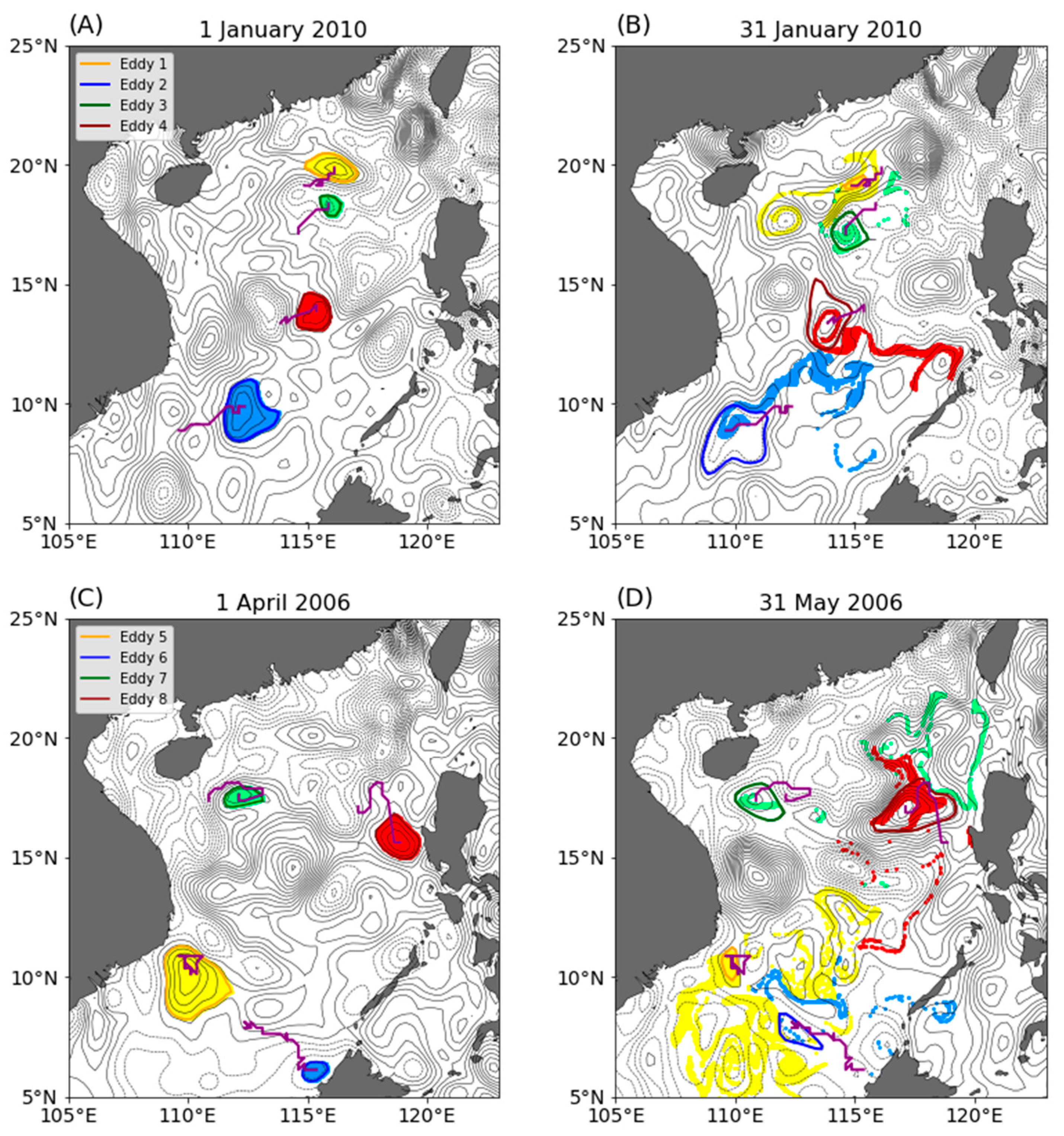
3.1. Features of SSH Eddies in the SCS

Before diagnosing eddy material transport, it is useful to understand the general features of SSH eddies in the SCS. From January 1993 to December 2015, a total number of 1751 eddies with a lifespan of more than 30 days are identified including 951 cyclonic and 800 anticyclonic eddies, implying that there are on average 6.3 eddies on each day, which is slightly less than the 9.1 eddies calculated by He et al. [10] due to the previously mentioned algorithm modification. Figure 3 shows the geographic distribution of the eddy genesis number, radius, amplitude, and zonal propagation speed on a 1° × 1° longitude–latitude grid. The value in each grid denotes the averaged information from all the eddy snapshots. Figure 3A shows that eddies can be formed in most regions of the SCS basin, but they are most common in two regions: the northeastern SCS and the southwest of Luzon Island, which may be attributed to eddy shedding from the Kuroshio [22,40] and local wind variations [41,42], respectively. Figure 3B demonstrates that the eddy radius ranges from 60 km to 120 km, and eddies in the southern SCS are generally larger than those in the northern SCS, which is consistent with the decrease in Rossby deformation radius with latitude [43]. Another noticeable feature is that the radii of eddies near the eastern boundary are smaller. The spatial distribution of eddy amplitude (Figure 3C) is different from that of the eddy radius. Two regions with high amplitude values are observed in the northeastern and western SCS, corresponding to regions with significant eddy kinetic energy (EKE, Figure 1B). The averaged zonal eddy propagation speed is calculated using the zonal eddy displacement distance and the eddy lifetime. Because of the beta effects, SSH eddies tend to move westward throughout the SCS basin [3,44].

A few recent studies [10,12,23] have estimated eddy mass transport in the SCS by multiplying eddy volume by eddy propagation speed, assuming that there is no fluid exchange between SSH eddies and their surrounding environment. To obtain some ideas of how leaky the SSH eddies in the SCS are, we first examine the coherent transport ability of SSH eddies using several random cases. Figure 4A,B show the movement of water particles initially seeded inside the SSH boundaries of four eddies, randomly selected on 1 January 2010. All four eddies last for more than 30 days from this date. During the following 30-day period, these four eddies with different radii all move westward (purple lines), and the water particles gradually escape from the eddy interior and move along with the local current. The leakiness of particles in Eddy 2 (blue) and Eddy 4 (red) both exceeds 90%, and the escaped particles generally move in opposite directions relative to the drifting eddies themselves. A similar picture is also found for four eddies that could live for more than 60 days (Figure 4C,D). Although some initial particles remain trapped by SSH eddy boundaries, the majority of them lost the coherence to join in the background flow. These individual eddy cases clearly demonstrate that SSH eddies in the SCS are quite leaky in their lifetimes and that there are frequent fluid exchanges across the SSH eddy boundary, a result consistent with the idealized numerical modeling study [33].

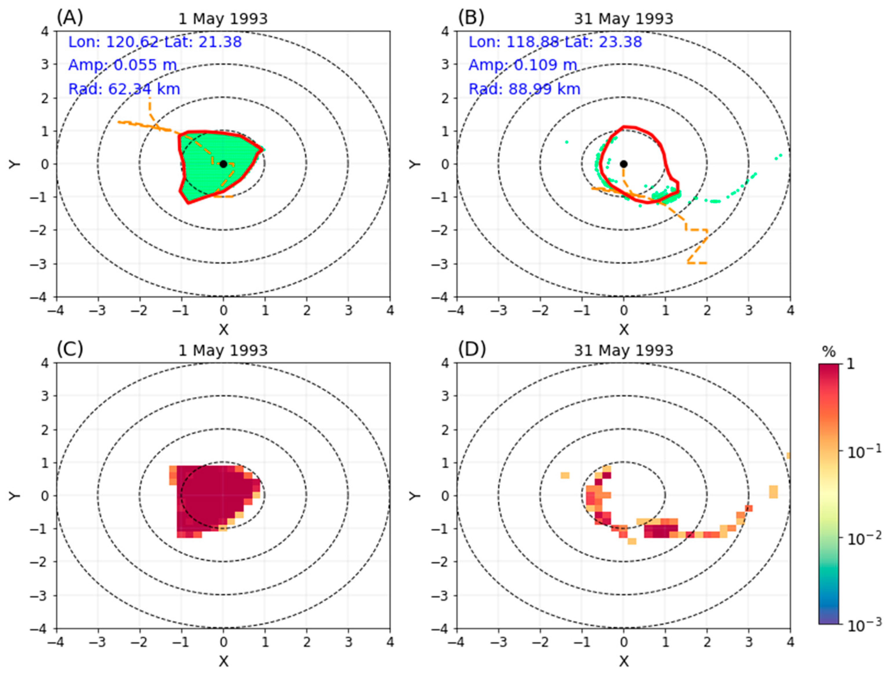
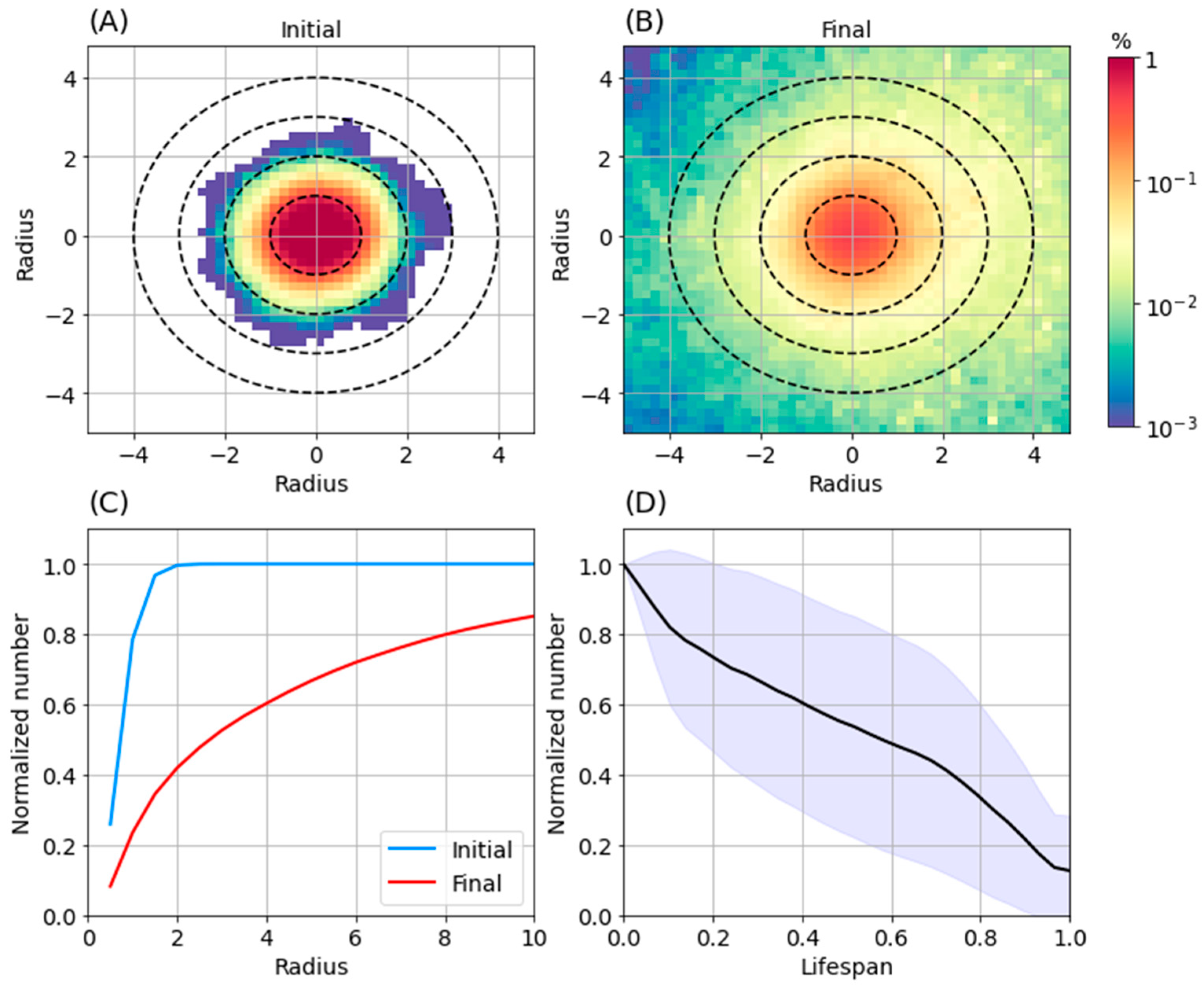
3.2. Statistical Analysis of SSH Eddy Leakage

To investigate the degree and spatial pattern of the SSH eddy leakage in the SCS, we carry out a statistical analysis of all the identified SSH eddies. First, eddy particle locations $\left(x,y\right)$ on the longitude–latitude coordinate are converted onto an eddy-centric coordinate $\left(X,Y\right)$ normalized by eddy radius $R$ and center $(x_c,y_c)$,

$$\left(X,Y\right)=\frac{\left(x,y\right)-(x_c,y_c)}{R}.$$

(2)

The new location $\left(X,Y\right)$ maintains the relative distance between the eddy center and the particle. Figure 5A,B shows the particle locations (green dots) in the normalized coordinates for a randomly-selected anticyclonic eddy on 1 May 1993 when particles are seeded inside its SSH boundary, and particle locations a month later on to 31 May. For this anticyclonic eddy, more than 90% of the initial particles have crossed the eddy SSH boundary after only 30 days, and the majority of the initial particles are not even located within four times the eddy radius (4R). If we further build a $0.2R\times 0.2R$ grid, the proportion of original eddy water in each grid $Q$ can be calculated by $Q=n/N_{total}$, where $n$ and $N_{total}$ indicate the particle number in a single grid and the total particle number for each eddy, respectively. Since the total number of particles is conserved, the sum of $Q$ is always 1. Figure 5C shows that at the initial time, the values of $Q$ in the eddy interior are close to 1%. It should be noted that this specific value $Q$ is determined by the grid resolution ($0.2R$); it is the subsequent variation and spatial distribution of $Q$ in the eddy lifespan that is of interest here. Figure 5D shows that after 30 days, the number of grids containing the initial eddy water becomes quite limited within 1R, and the value of $Q$ decreases by nearly one order of magnitude. In addition, some of the leaked initial particles are advected to the east side of the eddy center.

An advantage of the Eulerian identification method is that SSH eddies can be identified at any instantaneous time that the SLA data is available. For the Lagrangian identification method, due to the enormous amount of outputs from the LAVD calculations, Lagrangian particles with a resolution of 1/32° are only initialized on the first day of every month from January 1993 to December 2015, which means that the realistic initial date of SSH eddies may not match the date of Lagrangian particle release. In order to examine the leakage of SSH eddies using Lagrangian particles, we must first verify that the initial SSH eddy is fully covered by particles. For an SSH eddy, the first following release day is considered as its initial time and it will be used for the statistical analysis if it can survive for more than 20 days. The final time is determined from the last output day (a frequency of 10 days) during its lifespan. For example, the anticyclonic eddy in Figure 5 is generated on 18April 1993 and its duration is 47 days. The time interval from 1 May 1993 to 31 May 1993 is chosen to execute the related analysis. Despite the fact that this scheme might discard a small fraction of the eddy lifespan, it is an effective method for diagnosing the eddy leakage [33].

Figure 6 depicts the statistical distributions of $Q$ in the normalized coordinates for all eddies at the initial and final times, based on the method described above. It is shown that the averaged values of $Q$ within 1R are close to 1% at the initial time. Due to the fact that the shape of an SSH eddy is not always a perfect circle, some particles at the initial time are located outside of the 1R circle in the normalized coordinate, however, their $Q$ values are substantially smaller than those in the eddy interior. With the rapid escape of particles from SSH eddies, the values of $Q$ within 1R significantly decrease, and the leaked water moves along with the local currents. An intriguing aspect of the $Q$ value distribution is that there are more particles on the east side of the eddy than that on the west side at the final time due to the fact that most eddies propagate westward (Figure 3). This also indicates that particles leaked from SSH eddies are not carried coherently westward by the eddies and as a result, they show up on the east half of the eddy-centric coordinate. Figure 6C shows that all the particles a located within 2R from the eddy centers. At the final time, more than 60% of the particles are located outside of 2R, and only about 20% of the particles remain within the normalized eddy interior (1R).

Since the time intervals used in the above analysis may not always cover the whole lifespan of SSH eddies, here, we normalize these time intervals relative to the full length of eddy lifespan. For example, for the random eddy shown in Figure 5, the selected time interval corresponds to the normalized stage from 0.28 to 0.91. Figure 6D shows the average leakage trend for all eddies over the normalized lifespan. The initially trapped water by SSH eddies leaks at a nearly linear rate, with only less than 20% remaining inside the SSH boundary at the final time. The strong leakage could be explained by the Reynolds transport theorem [45]. When the velocity of the eddy boundary (SSH contour) does not always coincide with the fluid velocity in a two-dimensional eddy system, there will be active material flux across the boundary [33].

Having described the statistics of all eddies, we now present the differences between anticyclonic and cyclonic eddies. Figure 7 shows the spatial distributions of $Q$ at the final time and leakage trends as a function of the normalized lifespan for the two types of eddies. In addition to the aforementioned zonal asymmetry of $Q$ distribution, there is also an obvious meridional asymmetry of $Q$ for anticyclonic and cyclonic eddies. Higher values of $Q$ are found on the north side of anticyclonic eddies, and the opposite is true for cyclonic eddies. This result is likely due to the fact that anticyclonic (cyclonic) eddies tend to propagate equatorward (poleward) in the Northern Hemisphere [3], thereby leaving leaked particles behind on the north (south) side of the eddies. The numerical simulation [46] of eddy evolution and propagation corroborates these findings. Other than that, the two types of eddies have similar leakage trends, including both leakage degree (more than 80%) and rate. Our results suggest that, although the spatial distributions of leaked water are somewhat different between anticyclonic and cyclonic eddies, a common feature for all SSH eddies in the SCS is that they are highly leaky during their lifespans.

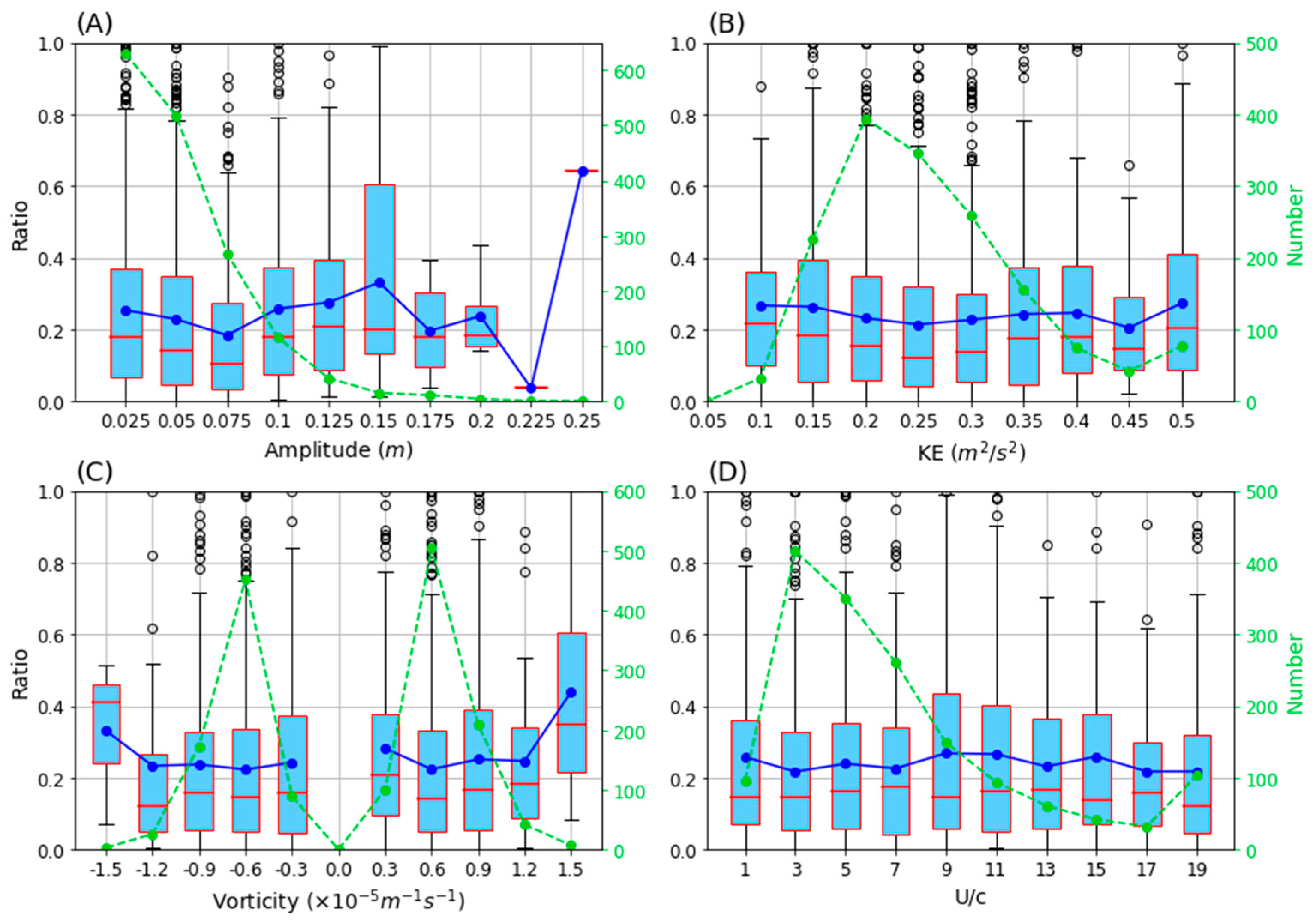
3.3. Dependence of Leakiness on Eddy Parameters

Eddies are often characterized by a number of parameters including amplitude (the absolute value of SSH difference between the eddy center and the boundary), radius, relative vorticity, kinetic energy, and so on. Does the degree of eddy leakage depend on any of these eddy parameters? To investigate this issue, six representative eddy parameters are selected.

Figure 8 shows the percentage of particles remaining inside SSH eddies at the final time as functions of eddy amplitude, kinetic energy, vorticity, and U/c. The SSH eddies are grouped by the specific value of parameters, and the distributions of eddies in each group are shown using a box-and-whisker diagram. The eddy number for different groups (green dashed line) is also displayed to exclude abnormal features associated with a small sample size. The eddy number in each group significantly decreases as the eddy amplitude increases from 0.025 m to 0.25 m, however, the leakage degree exhibits similar behavior except for the two groups with few eddies (Figure 8A). For all four eddy parameters, the median values of the percentage of particles remaining inside the SSH eddies are almost always smaller than 0.2, and the mean values vary between 0.2 and 0.3. Our results therefore show that the degree of leakage of SSH eddies is generally independent of parameters such as eddy amplitude, kinetic energy, vorticity, and U/c (Figure 8B–D). A value of U/c = 1 is often considered as a threshold above which the eddies are thought to be able to trap and translate fluid [3], but our results show that the values of U/c are not a good indicator of eddy trapping and coherent transport in the SCS. Estimates made based on the criteria of U/c > 1 are likely to strongly overestimate the degree of coherent eddy transport.

The degree of leakage of SSH eddies is found to be relatively sensitive to two other eddy parameters: duration and change of amplitude. Figure 9A shows that eddies with longer lifespans tend to lose more initial water than eddies with shorter lifespans, with the leakage ratio reaching more than 90% for eddies surviving longer than 180 days, indicating that it is difficult to maintain a coherent structure for eddies traveling a long distance. The change in eddy amplitude over a time interval is of interest here because it is a measure of the stage of eddy evolution. Positive (negative) values represent the growing (decaying) state of eddies, which generally corresponds to an increase (decrease) in eddy radius [33]. For two eddies of the same size at the initial time, the leakage degree of the growing eddy may be smaller than that of the decaying eddy because the boundary of a growing eddy is likely to expand over time, making it more likely to contain the particles. This potentially explains why in Figure 9B, the percentage of particles remaining inside SSH eddies increases with increasing amplitude change. The dependence of eddy trapping efficiency on stages of eddy growth/decay is worth further investigation, but is left for a future study.

3.4. Coherent and Incoherent Contributions to Total Eddy Transport

Having demonstrated that SSH eddies identified by the Eulerian method are far from coherent structures, we now turn to detecting actual coherent eddies based on the Lagrangian framework and examine the role of these eddies in material transport.

Figure 10 shows the initial and final locations of 30-day RCLVs generated on 1 September 2010 as well as 60-day RCLVs generated on 1 April 2006. An obvious feature is that the majority of RCLVs are initially placed around the local extremum of the SLA, but their size is much smaller than the outermost closed SLA contour, which has also been noticed by previous studies [27,33]. In August 2012, 15 coherent eddies are identified in the SCS, and they are able to maintain a coherent structure without significant leakage. Filamentary structures develop for several eddies because we use a relatively moderate parameter [47] in the eddy detection to avoid underestimating the number of coherent structures (see Appendix A). Despite this, only two 60-day coherent eddies are found in the whole SCS basin in this randomly selected time period, which means that the long-lived coherent eddies are relatively rare in the SCS.

From January 1993 to December 2015, there are 3239 30-day RCLVs and 516 60-day RCLVs identified in the SCS. Figure 11A shows the time series for the eddy number per month. The number of 30-day RCLVs typically ranges between 7 and 18 per month without any discernible seasonal or interannual signals. Since the number of 60-day RCLVs is typically less than 5 per month, we do not attempt to use an even longer detection period in this study. Although the identified SSH eddies (1751) are less than the Lagrangian eddies, SSH eddies have longer lifespans. We counte the total snapshot number of SSH eddies in each month and divide the number by 30, and then compare the value (green line in Figure 11A) with the number of 30-day RCLVs. It is observed that the number of SSH eddies calculated in this way also ranges between 7 and 18, indicating that the probability of occurrence for the two types of eddies is similar. However, they differ significantly in terms of eddy radius (Figure 11B). The radius of SSH eddies decreases with increasing latitude (from 5°N to 20°N) from 95 km to 77 km, with an average radius of 80.69 km. For 30-day and 60-day RCLVs, the radius does not vary significantly with latitude. The average radius of 30-day and 60-day RCLVs is 44.75 km and 44.68 km, respectively, approximately half of the size of SSH eddies. Previous numerical results [33] support the ratio observed here.

The absolute diffusivity is often used as a means to represent the fundamental properties of a turbulent flow [27,48,49]. The meridional component of the absolute diffusivity is defined as

$$K_{abs}=\frac{1}{2}\frac{\partial }{\partial t}\overline{{\left(y-y_0\right)}^2},$$

(3)

where $y$ is the meridional position of a particle initially released at $y_0$. The absolute diffusivity measures the growth rate of the absolute dispersion of all particles advected by the full flow field. In this study, we mainly focus on the eddy component of the full material transport, which can be measured by the relative diffusivity $K_{rel}$ after removing the effects of the mean flow in the Lagrangian frame [27,50],

$$K_{rel}=\frac{1}{2}\frac{\partial }{\partial t}\overline{{\left(y-\overline{y}\right)}^2},$$

(4)

where $\overline{y}$ is the averaged position of all particles released at $y_0$. In this study, the ensemble consists of all particles originating in the same month over 23 years. We calculate $K_{rel}$ for 12 months and then take an average in order to remove the effects of the seasonal basin-scale circulation in the SCS [7,8]. In addition, the material transport by eddies can be divided into two types: coherent (trapping) transport and incoherent (stirring) transport [27,51]. Since we know the behaviors of all Lagrangian particles, the contribution of coherent eddy transport to the total eddy flux can be estimated by introducing a masking function to determine whether particles are coherently trapped by eddies or not [27]. The coherent relative diffusivity is then defined as

$$K_{rel}^{CS}=\frac{1}{2}\frac{\partial }{\partial t}\overline{m{\left(y-\overline{y}\right)}^2},$$

(5)

where m is the masking function, which is 1 inside each Lagrangian eddy and 0 outside.

We now calculate the absolute diffusivity, relative diffusivity, and coherent relative diffusivity in zonal and meridional directions over a 30-day period (Figure 12). It should be noted that only 30-day RCLVs are considered in the calculation of coherent relative diffusivity. The value of $K_{abs}$ is close to 10,000 m²/s in both directions, and the value of $K_{rel}$ is between 5000 and 7000 m²/s. The difference between them indicates the contribution of the mean flow to the dispersion of Lagrangian particles. The zonal $K_{rel}^{CS}$ has a magnitude of about 200 m²/s, which is slightly higher than the meridional component due to the stronger zonal propagation of eddies. The most striking result here is that the magnitude of $K_{rel}^{CS}$ is much smaller than $K_{abs}$ and $K_{rel}$. The fraction of coherent eddy transport to the total eddy transport can be quantified via the ratio of $K_{rel}^{CS}$ to $K_{rel}$ (green line in Figure 12), which never exceeds 5% in both zonal and meridional directions. This small contribution of coherent eddy structures to the total eddy transport suggests that material transport by eddies in the SCS is primarily caused by incoherent motions (such as filamentation outside the eddy core), which is broadly consistent with the results in [27,32]. The emphasis here is on representing the comparison of coherent and incoherent motions in the SCS in order to update the traditional perception of the importance of coherent eddy transport.

4. Conclusions and Discussion

The complex dynamical conditions in the SCS lead to the generation of numerous mesoscale eddies, which play significant roles in oceanic processes via transporting heat, salt, and nutrients. A number of previous studies have attempted to estimate the degree of coherent transport by mesoscale eddies using observations and numerical simulations, but the majority of these studies are based on the Eulerian framework. Recent studies have shown that using the Eulerian method might strongly overestimate the coherent eddy transport [27,33]. The purpose of our study is to investigate the material transport by eddies in the SCS using the Lagrangian framework.

Unlike Eulerian methods, which depend on instantaneous fields at contiguous times, Lagrangian methods consider particle trajectories to organize the coherent structure. The large-scale operation of Lagrangian particles driven by observational data to detect coherent eddies has been reported in the eastern Pacific [27]. In a related work, we have extended this application to the global ocean in order to produce a Lagrangian eddy dataset. In this study, we focus on the eddy transport in the SCS by analyzing particles advected by the surface geostrophic current inferred from satellite altimeter data. An Eulerian method based on closed SSH contours and a Lagrangian method based on the LAVD technique are adopted to identify SSH eddies and RCLVs, respectively, from January 1993 to December 2015.

The spatial distributions of general features for SSH eddies in the SCS (such as amplitude, radius, etc.) are first examined, which are found comparable to previous studies. Lagrangian particles are then employed to investigate the leakiness of SSH eddies. Several random cases show that SSH eddies are highly leaky during their lifespans. The statistical features of leakage for all SSH eddies are then explored in an eddy-centric coordinate. The initial water inside SSH eddies tends to leak rapidly from the eddy interior, with less than 20% of the water trapped by the SSH boundary all the time. The leaked water is advected by the background flow, and would be likely to appear, on average, more frequently to the east of the eddy center due to the predominant westward propagation of eddies. The degree and rate of leakage for cyclonic and anticyclonic eddies are similar, but the spatial distribution of leaked water shows a meridional asymmetry due most likely to their opposite meridional propagation preferences. Furthermore, it is found that the leakage magnitude of SSH eddies does not depend on eddy parameters such as amplitude, kinetic energy, vorticity, and the nonlinearity parameter U/c. Our results indicate that high leakiness during eddy lifespan is a common feature of SSH eddies in the SCS and that the commonly used threshold of U/c > 1 is not a good indicator of eddy trapping and coherent transport.

The detected RCLVs are compared to SSH eddies in terms of eddy number and radius. From 1993 to 2015, there are approximately 7 to 18 30-day RCLVs every month, with a much lower number of 60-day RCLVs. Though the frequency of occurrence is similar for the two types of eddies, RCLVs are typically smaller in size than SSH eddies, with a ratio of radius of roughly 0.5. Several types of diffusivities are then calculated to quantify the contribution of the coherent eddy transport to the total eddy flux. Our key finding is that $K_{rel}^{cs}$, standing for the diffusive transport induced by coherent eddies, accounts for less than 5% of $K_{rel}$, the diffusive transport induced by the full eddying flow in both zonal and meridional directions. This indicates that the transport by coherent eddies provides a negligible contribution to the net eddy material transport in the SCS.

What may cause substantial leakage of SSH eddies in the SCS? The idealized numerical experiment of an isolated eddy [46] shows that most of the tracer originally inside of the eddy remains trapped by the SSH boundary after 675 days, which indicates that the SSH eddy is close to bea coherent structure and conforms to the conventional understanding. However, the statistical leakage of SSH eddies in an idealized ocean basin driven by constant wind forcing can reach about 50% after 30 days [33]. The primary difference between the above two numerical experiments is that the isolated eddy moves in a tranquil basin, whereas the latter involves a turbulent ocean. This suggests that the background flow can exert a large influence on the coherency of Eulerian eddies. The intricate multi-scale processes in the SCS such as the large-scale seasonal circulation, eddy–eddy interactions, Kuroshio intrusion, internal waves, and sub-mesoscale processes may be factors that lead to stronger leakage (80% in our calculation) than that found in the idealized model experiments. Recent observations have shown that the level of turbulent mixing is elevated in the periphery of mesoscale eddies [52], also providing reasonable evidence that the nonlinear effects may reduce the degree of coherent transport. Another factor that potentially causes high eddy leakage in the SCS is its complex topography including numerous islands and seamounts. Numerical simulations have shown that when encountering an island/seamount, the eddy behavior changes dramatically [53]. Physical processes and factors that influence eddy trapping efficiency is worth further investigation, and we plan to conduct a suite of numerical experiments in a future study to explore this issue.

In this study, the Lagrangian particles are advected by two-dimensional surface geostrophic currents derived from satellite altimeter data. As such, the effect of vertical motion on eddy coherent transport is not considered here. Due to the lack of observations of three-dimensional flow fields under the surface, research on the effect of vertical motions on eddy material transport will inevitably rely on numerical model simulations. Despite this caveat, the implications from this study are clear: Eulerian eddies are not coherent structures and are highly leaky, and therefore, previous studies based on Eulerian methods are likely to significantly overestimate coherent eddy transport in the SCS. Since coherent eddy transport only makes a small contribution to the total eddy transport in the SCS, more attention is required to understand material transport by incoherent motions in the future.

References

1. Wunsch, C.; Ferrari, R. Vertical mixing, energy, and the general circulation of the oceans. Annu. Rev. Fluid Mech. 2004, 36, 281–314. [Google Scholar] [CrossRef] [Green Version]
2. Fu, L.-L.; Chelton, D.; Le Traon, P.-Y.; Morrow, R. Eddy Dynamics From Satellite Altimetry. Oceanography 2010, 23, 14–25. [Google Scholar] [CrossRef] [Green Version]
3. Chelton, D.B.; Schlax, M.G.; Samelson, R.M. Global observations of nonlinear mesoscale eddies. Prog. Oceanogr. 2011, 91, 167–216. [Google Scholar] [CrossRef]
4. Jayne, S.R.; Marotzke, J. The dynamics of ocean heat transport variability. Rev. Geophys. 2001, 39, 385–411. [Google Scholar] [CrossRef] [Green Version]
5. Thompson, A.F.; Heywood, K.; Schmidtko, S.; Stewart, A. Eddy transport as a key component of the Antarctic overturning circulation. Nat. Geosci. 2014, 7, 879–884. [Google Scholar] [CrossRef]
6. Busecke, J.J.M.; Abernathey, R.P. Ocean mesoscale mixing linked to climate variability. Sci. Adv. 2019, 5, eaav5014. [Google Scholar] [CrossRef] [Green Version]
7. Liu, Q.; Kaneko, A.; Jilan, S. Recent progress in studies of the South China Sea circulation. J. Oceanogr. 2008, 64, 753–762. [Google Scholar] [CrossRef]
8. Zheng, Q.; Hu, J.; Ho, C.-R.; Xie, L. Advances in Research of Regional Oceanography of the South China Sea: Overview; World Scientific Publishing Company: Singapore, 2020; pp. 1–18. [Google Scholar] [CrossRef]
9. Chen, G.; Hou, Y.; Chu, X. Mesoscale eddies in the South China Sea: Mean properties, spatiotemporal variability, and impact on thermohaline structure. J. Geophys. Res. Ocean. 2011, 116, 711–720. [Google Scholar] [CrossRef]
10. He, Q.; Zhan, H.; Cai, S.; He, Y.; Huang, G.; Zhan, W. A New Assessment of Mesoscale Eddies in the South China Sea: Surface Features, Three-Dimensional Structures, and Thermohaline Transports. J. Geophys. Res. Ocean. 2018, 123, 4906–4929. [Google Scholar] [CrossRef]
11. Liu, Y.; Dong, C.; Liu, X.; Dong, J. Antisymmetry of oceanic eddies across the Kuroshio over a shelfbreak. Sci. Rep. 2017, 7, 6761. [Google Scholar] [CrossRef] [Green Version]
12. Ding, R.; Xuan, J.; Zhang, T.; Zhou, L.; Zhou, F.; Meng, Q.; Kang, I.-S. Eddy-induced Heat Transport in the South China Sea. J. Phys. Oceanogr. 2021, 51, 2329–2349. [Google Scholar] [CrossRef]
13. Haller, G. Lagrangian coherent structures. Annu. Rev. Fluid Mech. 2015, 47, 137–162. [Google Scholar] [CrossRef] [Green Version]
14. Dong, C.; McWilliams, J.C.; Liu, Y.; Chen, D. Global heat and salt transports by eddy movement. Nat. Commun. 2014, 5, 3294. [Google Scholar] [CrossRef] [PubMed] [Green Version]
15. Zhang, Z.; Wang, W.; Qiu, B. Oceanic mass transport by mesoscale eddies. Science 2014, 345, 322–324. [Google Scholar] [CrossRef] [PubMed]
16. Wang, G.; Su, J.; Chu, P. Mesoscale eddies in the South China Sea observed with altimeter data. Geophys. Res. Lett. 2003, 30. [Google Scholar] [CrossRef] [Green Version]
17. Xiu, P.; Chai, F.; Shi, L.; Xue, H.; Chao, Y. A census of eddy activities in the South China Sea during 1993–2007. J. Geophys. Res. Ocean. 2010, 115. [Google Scholar] [CrossRef] [Green Version]
18. Hu, J.; Gan, J.; Sun, Z.; Zhu, J.; Dai, M. Observed three-dimensional structure of a cold eddy in the southwestern South China Sea. J. Geophys. Res. Ocean. 2011, 116. [Google Scholar] [CrossRef]
19. Lin, X.; Dong, C.; Chen, D.; Liu, Y.; Yang, J.; Zou, B.; Guan, Y. Three-dimensional properties of mesoscale eddies in the South China Sea based on eddy-resolving model output. Deep Sea Res. Part I: Oceanogr. Res. Pap. 2015, 99, 46–64. [Google Scholar] [CrossRef]
20. Zhang, Y.; Liu, Z.; Zhao, Y.; Wang, W.; Li, J.; Xu, J. Mesoscale eddies transport deep-sea sediments. Sci. Rep. 2014, 4, 5937. [Google Scholar] [CrossRef]
21. Wang, X.; Li, W.; Qi, Y.; Han, G. Heat, salt and volume transports by eddies in the vicinity of the Luzon Strait. Deep Sea Res. Part I Oceanogr. Res. Pap. 2011, 61, 21–33. [Google Scholar] [CrossRef]
22. Zhang, Z.; Zhao, W.; Qiu, B.; Tian, J. Anticyclonic Eddy Sheddings from Kuroshio Loop and the Accompanying Cyclonic Eddy in the Northeastern South China Sea. J. Phys. Oceanogr. 2017, 47, 1243–1259. [Google Scholar] [CrossRef] [Green Version]
23. Yang, Y.; Zeng, L.; Wang, Q. How Much Heat and Salt Are Transported Into the South China Sea by Mesoscale Eddies? Earth’s Futur. 2021, 9, e2020EF001857. [Google Scholar] [CrossRef]
24. Okubo, A. Horizontal dispersion of floatable particles in the vicinity of velocity singularities such as convergences. Deep Sea Res. Oceanogr. Abstr. 1970, 17, 445–454. [Google Scholar] [CrossRef]
25. Weiss, J. The dynamics of enstrophy transfer in two-dimensional hydrodynamics. Phys. D Nonlinear Phenom. 1991, 48, 273–294. [Google Scholar] [CrossRef]
26. Nencioli, F.; Dong, C.; Dickey, T.; Washburn, L.; McWilliams, J.C. A Vector Geometry–Based Eddy Detection Algorithm and Its Application to a High-Resolution Numerical Model Product and High-Frequency Radar Surface Velocities in the Southern California Bight. J. Atmos. Ocean. Technol. 2010, 27, 564–579. [Google Scholar] [CrossRef]
27. Abernathey, R.; Haller, G. Transport by Lagrangian Vortices in the Eastern Pacific. J. Phys. Oceanogr. 2018, 48, 667–685. [Google Scholar] [CrossRef] [Green Version]
28. Shadden, S.C.; Lekien, F.; Marsden, J.E. Definition and properties of Lagrangian coherent structures from finite-time Lyapunov exponents in two-dimensional aperiodic flows. Phys. D Nonlinear Phenom. 2005, 212, 271–304. [Google Scholar] [CrossRef]
29. D’Ovidio, F.; Isern-Fontanet, J.; López, C.; Hernández-García, E.; García-Ladona, E. Comparison between Eulerian diagnostics and finite-size Lyapunov exponents computed from altimetry in the Algerian basin. Deep Sea Res. Part I Oceanogr. Res. Pap. 2009, 56, 15–31. [Google Scholar] [CrossRef] [Green Version]
30. Haller, G.; Hadjighasem, A.; Farazmand, M.; Huhn, F. Defining coherent vortices objectively from the vorticity. J. Fluid Mech. 2016, 795, 136–173. [Google Scholar] [CrossRef] [Green Version]
31. Haller, G.; Beron-Vera, F.J. Coherent Lagrangian vortices: The black holes of turbulence. J. Fluid Mech. 2013, 731. [Google Scholar] [CrossRef] [Green Version]
32. Wang, Y.; Olascoaga, M.J.; Beron-Vera, F.J. Coherent water transport across the South Atlantic. Geophys. Res. Lett. 2015, 42, 4072–4079. [Google Scholar] [CrossRef] [Green Version]
33. Liu, T.; Abernathey, R.; Sinha, A.; Chen, D. Quantifying Eulerian Eddy Leakiness in an Idealized Model. J. Geophys. Res. Ocean. 2019, 124, 8869–8886. [Google Scholar] [CrossRef] [Green Version]
34. Adcroft, A.; Campin, J.M.; Doddridge, S.D.; Evangelinos, C.; Ferreira, D.; Follows, M.; Scott, J. MITgcm documentation. Release Checkp. 2018, 19, 67a-12-gbf23121. [Google Scholar]
35. Abernathey, R.P.; Marshall, J. Global surface eddy diffusivities derived from satellite altimetry. J. Geophys. Res. Ocean. 2013, 118, 901–916. [Google Scholar] [CrossRef]
36. He, Y.; Xie, J.; Cai, S. Interannual variability of winter eddy patterns in the eastern South China Sea. Geophys. Res. Lett. 2016, 43, 5185–5193. [Google Scholar] [CrossRef]
37. He, Y.; Feng, M.; Xie, J.; He, Q.; Liu, J.; Xu, J.; Chen, Z.; Zhang, Y.; Cai, S. Revisit the Vertical Structure of the Eddies and Eddy-Induced Transport in the Leeuwin Current System. J. Geophys. Res. Ocean. 2021, 126, e2020JC016556. [Google Scholar] [CrossRef]
38. Faghmous, J.H.; Frenger, I.; Yao, Y.; Warmka, R.; Lindell, A.; Kumar, V. A daily global mesoscale ocean eddy dataset from satellite altimetry. Sci. Data 2015, 2, 150028. [Google Scholar] [CrossRef] [Green Version]
39. Zhang, W.; Wolfe, C.L.P.; Abernathey, R. Role of Surface-Layer Coherent Eddies in Potential Vorticity Transport in Quasigeostrophic Turbulence Driven by Eastward Shear. Fluids 2019, 5, 2. [Google Scholar] [CrossRef] [Green Version]
40. Nan, F.; Xue, H.; Chai, F.; Shi, L.; Shi, M.; Guo, P. Identification of different types of Kuroshio intrusion into the South China Sea. Ocean Dyn. 2011, 61, 1291–1304. [Google Scholar] [CrossRef]
41. Wang, G.; Chen, D.; Su, J. Winter Eddy Genesis in the Eastern South China Sea due to Orographic Wind Jets. J. Phys. Oceanogr. 2008, 38, 726–732. [Google Scholar] [CrossRef]
42. Cheng, X.; Xie, S.-P.; Du, Y.; Wang, J.; Chen, X.; Wang, J. Interannual-to-decadal variability and trends of sea level in the South China Sea. Clim. Dyn. 2015, 46, 3113–3126. [Google Scholar] [CrossRef] [Green Version]
43. Chelton, D.B.; DeSzoeke, R.A.; Schlax, M.G.; El Naggar, K.; Siwertz, N. Geographical variability of the first baro-clinic Rossby radius of deformation. J. Phys. Oceanogr. 1998, 28, 433–460. [Google Scholar] [CrossRef]
44. Huang, R.; Xie, L.; Zheng, Q.; Li, M.; Bai, P.; Tan, K. Statistical analysis of mesoscale eddy propagation velocity in the South China Sea deep basin. Acta Oceanol. Sin. 2020, 39, 91–102. [Google Scholar] [CrossRef]
45. Reynolds, O. The Sub-Mechanics of the Universe; University Press: Cambridge, UK, 1903; Volume 3. [Google Scholar]
46. Early, J.J.; Samelson, R.M.; Chelton, D.B. The Evolution and Propagation of Quasigeostrophic Ocean Eddies. J. Phys. Oceanogr. 2011, 41, 1535–1555. [Google Scholar] [CrossRef]
47. Tarshish, N.; Abernathey, R.; Zhang, C.; Dufour, C.O.; Frenger, I.; Griffies, S. Identifying Lagrangian coherent vortices in a mesoscale ocean model. Ocean Model. 2018, 130, 15–28. [Google Scholar] [CrossRef]
48. LaCasce, J. Statistics from Lagrangian observations. Prog. Oceanogr. 2008, 77, 1–29. [Google Scholar] [CrossRef]
49. Klocker, A.; Ferrari, R.; LaCasce, J.H. Estimating Suppression of Eddy Mixing by Mean Flows. J. Phys. Oceanogr. 2012, 42, 1566–1576. [Google Scholar] [CrossRef] [Green Version]
50. Bennett, A.F. Relative Dispersion: Local and Nonlocal Dynamics. J. Atmos. Sci. 1984, 41, 1881–1886. [Google Scholar] [CrossRef] [Green Version]
51. Frenger, I.; Münnich, M.; Gruber, N.; Knutti, R. Southern Ocean eddy phenomenology. J. Geophys. Res. Ocean. 2015, 120, 7413–7449. [Google Scholar] [CrossRef] [Green Version]
52. Yang, Q.; Zhao, W.; Liang, X.; Dong, J.; Tian, J. Elevated Mixing in the Periphery of Mesoscale Eddies in the South China Sea. J. Phys. Oceanogr. 2017, 47, 895–907. [Google Scholar] [CrossRef]
53. Yang, S.; Xing, J.; Chen, D.; Chen, S. A modelling study of eddy-splitting by an island/seamount. Ocean Sci. 2017, 13, 837–849. [Google Scholar] [CrossRef] [Green Version]
Figure 1. Climatological (A) surface geostrophic currents (black vectors) and their speed (colors); (B) surface eddy kinetic energy (colors) in the SCS. The black contour in (B) indicates the 200 m isobath.
Remotesensing 14 01690 g001
Figure 2. (A) The initial latitude of Lagrangian particles released around the SCS on 1 January 2006. (B) The meridional displacement (in degree) of these particles after 180 days. (C) A 30-day LAVD field.
Remotesensing 14 01690 g002
Figure 3. Geographic distributions of the eddy (A) genesis number, (B) radius, (C) amplitude, and (D) zonal propagation speed on a 1° × 1° longitude–latitude grid in the SCS from January 1993 to 2015. The black contour in each panel denotes the 200 m isobath.
Remotesensing 14 01690 g003
Figure 4. The initial (left panels) and final (right panels) particle locations of randomly selected eddies that live for longer than (A,B) 30 and (C,D) 60 days. Colored contours are eddy boundaries defined by SSH contours. Colored dots represent the initial particles inside the eddy boundaries. Purple lines indicate eddy center trajectories.
Remotesensing 14 01690 g004
Figure 5. (A,B) Particle locations (green dots) and (C,D) distributions of Q in the normalized coordinate for a randomly-selected anticyclonic eddy at the initial and final times. Red contours represent SSH eddy boundaries. The eddy trajectory in the lifespan is denoted by the yellow dashed lines. Q is a measure of the proportion of initial eddy particles in each 0.2 R × 0.2 R grid.
Remotesensing 14 01690 g005
Figure 6. Statistical distributions of Q in the normalized coordinates for all eddies at the (A) initial and (B) final times. (C) Cumulative ratio of initial particles within a given distance normalized by eddy radius. (D) Leakage trend for all eddies during the normalized lifespan, with color shading representing one standard deviation of the mean over all samples.
Remotesensing 14 01690 g006
Figure 7. (A,B) Spatial distributions of Q at the final time and (C,D) leakage trends during the normalized lifespan for anticyclonic (left panels) and cyclonic (right panels) eddies. Color shading in (C,D) represents one standard deviation of the mean over all samples.
Remotesensing 14 01690 g007
Figure 8. The percentage of particles remaining inside SSH eddies at the final time as functions of eddy (A) amplitude, (B) kinetic energy, (C) vorticity, and (D) U/c. Statistics of all eddies for different parameters are shown using a box-and-whisker plot. The red line indicates the median. The blue box covers the 25th to 75th percentiles of the distribution. The black whiskers indicate the 5th to 95th percentiles. The black circle symbols indicate the outliers beyond the 5th to 95th percentiles. The green dashed line indicates eddy numbers for different values of eddy parameters. The blue solid line represents the mean of each group.
Remotesensing 14 01690 g008
Figure 9. As in Figure 8, but for (A) eddy duration and (B) change of amplitude.
Remotesensing 14 01690 g009
Figure 10. Initial (red dots) and final (blue dots) locations for (A) 30-day and (B) 60-day RCLVs in two random time intervals. The purple line indicates the eddy trajectory. The black contours represent the SLA on the initial date with an interval of 2 cm.
Remotesensing 14 01690 g010
Figure 11. (A) Numbers of 30-day (red line) and 60-day (blue line) RCLVs per month from 1993 to 2015, with the total snapshot number of SSH eddies per month (divided by 30) as shown by the green line. (B) The radii of RCLVs and SSH eddies as a function of latitude. The error bar represents one standard deviation of the mean over all samples in a 1.5° bin.
Remotesensing 14 01690 g011
Figure 12. Absolute diffusivity (black line), relative diffusivity (red line), and coherent relative diffusivity (blue line) in (A) zonal and (B) meridional directions over 30 days, with the green line indicating the ratio of coherent relative diffusivity to the relative diffusivity. Note the non-uniform scale on the y axis.
Remotesensing 14 01690 g012
Publisher’s Note: MDPI stays neutral with regard to jurisdictional claims in published maps and institutional affiliations.