Article

Comparison of Scanning LiDAR with Other Remote Sensing Measurements and Transport Model Predictions for a Saharan Dust Case

1
Institute of Meteorology and Climate Research, Karlsruhe Institute of Technology, 76344 Eggenstein-Leopoldshafen, Germany
2
Deutscher Wetterdienst (DWD), Frankfurter Str. 135, 63067 Offenbach am Main, Germany
*
Author to whom correspondence should be addressed.
Remote Sens. 2022, 14(7), 1693; https://doi.org/10.3390/rs14071693
Submission received: 5 February 2022 / Revised: 2 March 2022 / Accepted: 29 March 2022 / Published: 31 March 2022
(This article belongs to the Special Issue Selected Papers of the European Lidar Conference)

Abstract

:
The evolution and the properties of a Saharan dust plume were studied near the city of Karlsruhe in southwest Germany (8.4298°E, 49.0953°N) from 7 to 9 April 2018, combining a scanning LiDAR (90°, 30°), a vertically pointing LiDAR (90°), a sun photometer, and the transport model ICON-ART. Based on this Saharan dust case, we discuss the advantages of a scanning aerosol LiDAR and validate a method to determine LiDAR ratios independently. The LiDAR measurements at 355 nm showed that the dust particles had backscatter coefficients of 0.86 ± 0.14 Mm 1 sr 1 , extinction coefficients of 40 ± 0.8 Mm 1 , a LiDAR ratio of 46 ± 5 sr, and a linear particle depolarisation ratio of 0.27 ± 0.023. These values are in good agreement with those obtained in previous studies of Saharan dust plumes in Western Europe. Compared to the remote sensing measurements, the transport model predicted the plume arrival time, its layer height, and its structure quite well. The comparison of dust plume backscatter values from the ICON-ART model and observations for two days showed a correlation with a slope of 0.9 ± 0.1 at 355 nm. This work will be useful for future studies to characterise aerosol particles employing scanning LiDARs.

1. Introduction

Atmospheric dust has a significant impact on the Earth’s climate system, but the impacts remain highly uncertain [1]. These uncertainties are attributed to the larger spatial–temporal variability of aerosol dust and its complex interaction with atmosphere constituents, radiation, and clouds [2]. Besides, dust particles can participate in cloud formation as Cloud Condensation Nuclei (CCNs) and Ice-Nucleating Particles (INPs), and these clouds can redistribute solar radiation [3,4,5,6,7,8]. Furthermore, dust plumes can modify cloud microphysics and may even change precipitation distributions [9,10]. Hence, simultaneous observation of clouds and dust plumes can help unravel the details of dust–cloud interaction processes.
Understanding the distribution and the properties of dust is the key to quantifying radiative forcing [11]. For decades, satellites have been used to study the properties and transportation of dust around the globe. However, their data still have limitations, especially concerning the characterisation of the vertical structure at a high resolution of dust plumes for passive sensors aboard satellites (e.g., Meteosat, Terra and Aqua) and cannot not obtain continuous datasets at one place for polar orbit satellites (e.g., Terra and Aqua, CALIPSO). In addition, satellite data still have limitations compared to ground-based active remote sensing methods, e.g., concerning the characterisation of the structures of dust plumes especially for low aerosol particle concentrations [12].
Various studies characterised Saharan dust near the sources, as well as during and after long-range transport. Freudenthaler et al. [13] reported pure Saharan dust depolarisation ratio profiling at several wavelengths during the Saharan Mineral Dust Experiment (SAMUM) 2006. Kanitz et al. [14] observed Saharan dust with shipborne LiDAR from 60° to 20°W along 14.5°N. Soupiona et al. [15] studied dust properties and their impact on radiative forcing over the northern Mediterranean region based on EARLINET observations. The three-dimensional evolution of Saharan dust transport toward Europe was studied based on a nine-year EARLINET-optimised CALIPSO dataset [16]. The Copernicus Atmosphere Monitoring Service (CAMS) forecast systems simulated the aerosol transport events over Europe during the 2017 storm Ophelia and validated these results with passive (MODIS: Moderate Resolution Imaging Spectroradiometer aboard Terra and Aqua) and active (CALIOP/CALIPSO: Cloud-Aerosol LIDAR with Orthogonal Polarization aboard Cloud-Aerosol LiDAR and Infrared Pathfinder Satellite Observations) satellite sensors, as well as ground-based measurements (EMEP: European Monitoring and Evaluation Programme) [17]. Osborne et al. [18] compared model simulations with ground-based remote sensing measurements (LiDAR and sun photometer network). A comparison of dust observations by LiDAR and the BSC-DREAM8b model results was studied by Mona et al. [19]. In addition, intensive field campaigns such as SAMUM investigated the relation among the chemical composition, shape, morphology, size distribution, and optical effects of dust particles with emphasis on vertical profiling of dust optical properties. The SAMUM experiment consisted of two campaigns—SAMUM-1 and SAMUM-2. SAMUM-1 was mostly conducted at Ouarzazate (30.9°N, 6.9°W, 1133 m a.s.l.) and Tinfou near Zagora (30.24°N and 5.61°W about 730m a.s.l.) in 2006 and SAMUM-2 was conducted at Praia (Sao Vicente island, Cape Verde, 14.9°N, 23.5°W, 75 m a.s.l.) in 2008 [13,20,21,22,23,24]. By these field campaigns, the chemical/mineralogical composition, microphysical characteristics, and optical properties of Saharan dust were studied. The chemical composition is beyond the scope of this paper. Here, we briefly summarise the latter two characteristics. On the African continent, particles with diameters significantly larger than 10 μ m were observed, e.g., during the SAMUM-1 study. However, in 80% of the cases, the measured particle diameters were below 40 μ m. During SAMUM-2, the mean dust particle diameter was significantly smaller than during SAMUM-1 [24,25,26]. This phenomenon is related to large particles falling out of the plume during long transportation and the observation station of SAMUM-2 being further from the dust source region [27]. The authors also found that Saharan dust particles observed during SAMUM-1 and SAMUM-2 were almost non-hygroscopic [28]. In addition, the complex refractive index of pure dust, the Single Scattering Albedo (SSA) at different wavelengths, and the Angstrom Exponents (AE) were obtained with remote sensing and airborne measurements [20,23,29]. Recently, synergistic methods including ground-based, airborne, remote sensing, and numerical modelling have become important ways to better understand dust plume evolutions [30,31,32].
Aerosol elastic scattering LiDAR is widely used for aerosol and cloud research [33] as it can provide detailed information with high spatial and temporal resolution. However, retrieving the backscatter coefficient from this kind of LiDAR data requires assumptions of LiDAR ratios and reference values [34,35]. The LiDAR ratio is an import parameter for LiDAR research as it can not only help to determine extinction coefficients, but also can be used in other aspects such as aerosol typing [36,37,38]. However, determining LiDAR ratios is not easy. One of the most widely used technologies is the Raman LiDAR [39]. However, this technology is mainly limited to night time measurements due to the weak intensities of Raman scattering. Another widely used technology is the High-Spectral-Resolution LiDAR (HSRL) [40], which uses a narrow-band filter (e.g., atom or molecule filter) to separate signals from molecule and particle backscatter. However, this kind of filter can only work at specific wavelengths. For example, the most commonly used filter is the iodine cell, which only works at 532 nm [41]. Recently, an HSRL that uses an interferometer as a filter was deployed at other wavelengths. The recently launched Doppler wind LiDAR, ALADIN, uses this technology to measure tropospheric wind profiles on a global scale, but can also obtain vertical aerosol profiles [42]. However, this technology is still not widely used due to the complex configurations of this kind of system. The aerosol optical depth measured by a sun photometer can also be used to constrain the LiDAR retrieval, thus helping us obtain column-averaged LiDAR ratios [43].
Scanning aerosol LiDARs have been used to determine three-dimensional aerosol distributions [44,45,46,47] and particle orientations [48]. Furthermore, a method using multiple angles, e.g., based on scanning aerosol LiDAR measurements, was proposed to retrieve extinction coefficients independently in horizontal homogeneous atmospheres [49,50]. The uncertainties of this method applied for inhomogeneous atmospheres and an improved method for poorly stratified atmospheres were also discussed [51,52,53]. This method has the advantage of retrieving extinction coefficients from elastic LiDAR measurements without assumptions of LiDAR ratios for the elastic LiDAR. Another better way to obtain extinction coefficients from elastic LiDAR measurements is via the Klett–Fernald method with a known LiDAR ratio. However, to the best of our knowledge, there is no method to retrieve LiDAR ratios directly from elastic LiDAR measurements.
Sun photometers can also be used to infer wavelength-dependent optical and microphysical properties of aerosols from observing direct and diffuse solar radiation [54,55]. The ground-based sun photometer aerosol network AERONET (AErosol RObotic NETwork) provides a long-term, continuous, and readily accessible public domain database for aerosol research [54].
Various global and regional transport models have been developed, and many of them can simulate the transport, transformation, and properties of aerosol particles. Examples of such models are the general circulation model, ECHAM-HAMMOZ [56,57], ECHAM/MESSy Atmospheric Chemistry (EMAC) [58,59,60], the Whole Atmosphere Community Climate Model (WACCM) [61,62], the Weather Research and Forecasting (WRF) model coupled with Chemistry (WRF/Chem) [63], the CONsortium for small-scale MOdeling (COSMO) and its extension Aerosol and Reactive Trace gases (ART) [64], and its successor, ICOsahedral Nonhydrostatic (ICON), and its extension Aerosol and Reactive Trace gases (ART) [65,66]. Special focus has been on mineral dust due to its strong impact on atmospheric radiative forcing [1]. A three-dimensional mineral dust model has been developed to study its impact on the radiative balance of the atmosphere [67]. Recently, various models such as CAMS [68], WRF/Chem [69], EMAC [70], COSMO-ART [64,71], and ICON-ART [65,72,73] have been used to predict mineral dust plumes. A multi-model forecast comparison is available by the Sand and Dust Storm Warning Advisory and Assessment System [74], a program of the World Meteorological Organisation (WMO).
For the dust event that occurred in April 2018, we collected a comprehensive set of data and compared it with a global transport model simulation to understand the distribution and evolution of dust near the city of Karlsruhe, in southwest Germany. Two LiDAR systems and a sun photometer were used to investigate the dust event employing different retrieval methods. The major objective was to quantify the uncertainties of different measurement and retrieval methods including a demonstration of how useful scanning LiDAR measurements can be in addition to vertical LiDAR and sun photometer data and what kind of understanding of the aerosol properties can be achieved by combining the different measurement techniques. Furthermore, we compared these observational data with predictions calculated by the state-of-the-art transport model, the ICON-ART model, to understand the distribution and evolution of dust near the city of Karlsruhe, in southwest Germany.
This paper is organised as follows. Section 2 describes the remote sensing methods and the model simulations. Details of the dust observations and dust properties are discussed in Section 3 including a comparison of the different remote sensing methods, as well as how they compare to the model predictions. In the final section, we provide some conclusions.

2. Methods

Two LiDAR systems were used in this study, a vertically pointing system called the Deutscher Wetterdienst-Depolarization Raman LiDAR (DWD-DELiRA (LR111-D200, Raymetrics Inc.)) and a spatially scanning system called the Karlsruhe scanning aerosol LiDAR (KASCAL (LR111-ESS-D200, Raymetrics Inc. Athens, Greece)). Both have an emission wavelength of 355 nm and are equipped with elastic, depolarisation, and Raman channels, hence providing profiles of extinction coefficients, particle backscatter coefficients, and depolarisation ratios. Besides, a sun photometer (CE-318, CIMEL, Holben et al. [54]) provides the wavelength-dependent AOD, Angstrom exponent, under clear sky via inversion, Aerosol Size Distributions (ASDs), and SSA. To predict the dust transport and distribution, the online coupled model system ICON-ART [65] was used. The model system is running in quasi-operational mode by Deutscher Wetterdienst (DWD).

2.1. Remote Sensing Instruments

For this observation campaign, the KASCAL and DWD-DELiRA LiDAR systems were deployed on the campus north of the Karlsruhe Institute of Technology (8.4298° E, 49.0953° N, 119 m above sea level). The KASCAL is operated by the Institute of Meteorology and Climate Research (IMK-AAF) at the Karlsruhe Institute of Technology and the DWD-DELIRA by the Deutscher Wetterdienst (DWD). The horizontal distance of the two LiDAR systems was 500 m. The sun photometer was installed at a roof between both LiDARs. The KASCAL LiDAR system is a mobile scanning system with an emission wavelength of 355 nm. The laser pulse energy and repetition frequency are 32 mJ and 20 Hz, respectively. The laser head, a 200 mm telescope, and LiDAR signal detection units are mounted on a rotating platform allowing zenith angles from −7º to 90º and azimuth angles from 0º to 360º. The overlap range of both LiDAR systems is 255 m, and the overlap correction for the KASCAL LiDAR was performed with horizontal measurements assuming horizontal homogeneous conditions. The overlap correction for the DWD-DELIRA was performed by comparing with scanning aerosol LiDAR. This KASCAL LiDAR works automatically, time-controlled, and continuously via software developed by Raymetrics Inc. [75,76]. The fixed vertically pointing LiDAR (DWD-DELiRA) has a laser energy power of 50–55 mJ at an emission wavelength of 355 nm and a 300 mm telescope area, as well as the same detection channels as the scanning LiDAR system.
For the data analysis and calibration of the system, we followed the quality standards of the European Aerosol Research LiDAR Network (EARLINET) [77]. The quality of the retrieval method was studied by EARLINET. The developed calculus modules, EARLINET Single Calculus Chain (SCC), show that the mean relative deviation is 10% (15%) for the Raman (Klett–Fernald) backscatter coefficient method and 15 % for Raman extinction coefficient retrieval [78]. Further, for optical depths τ ≤ 5 and SNR = 10, the estimated relative error is below 10%; for optical depths τ ≤ 5 and LiDAR ratio errors of 10%, the estimated error is below approximately 4% [79]. The uncertainties given in this paper include standard deviations from repeated profile measurements, which include both systematic LiDAR uncertainties and the variability of the atmosphere. For the data analysis in this Saharan dust case, Hamming window filters whose window length is 75 m (10 bins) were applied to raw LiDAR signals firstly. Then, extinction and backscatter coefficients at 355 nm were both calculated from the elastic channel using the Klett–Fernald method [34,35] and were also calculated from the elastic and Raman channels [80]. For extinction coefficients calculated with the Raman method, Hamming window filters with window lengths of 300 m (40 bins) were applied to the Raman signals, and subsequently, the retrievals were performed with an average vertical resolution of 150 m. Please note that the Raman data are only available for night time measurements. We compared our data analysis algorithm with the Single Calculus Chain (SCC) code (EARLINET) and the Raymeterics code and obtained consistent results. For the backscatter coefficients retrieved based on the Klett–Fernald method, we only show the results for periods free of clouds as the presence of clouds makes it very difficult to choose reasonable reference values for the retrieval methods. Particle depolarisation was calculated as suggested by Freudenthaler et al. [13]:
δ p = ( 1 + δ m ) δ v R ( 1 + δ v ) δ m ( 1 + δ m ) R ( 1 + δ v )
Here, δ m is the depolarisation ratio of gas molecules, which was assumed to be 0.004 in this paper according to Behrendt and Nakamura [81], δ v is the volume depolarisation ratio, and R is the backscatter ratio:
R = β p + β m β m
Here, β p is the backscatter coefficient of particles and β m is the backscatter coefficient of molecules.
The extinction coefficients and LiDAR ratios can also be retrieved using a multiangle method [49,50]. Additionally, we found that LiDAR ratios can be retrieved from elastic LiDAR signals independently. Although retrieval of LiDAR ratios is straightforward with known extinction coefficients based on the LiDAR equation, to the best of our knowledge, there is no report about retrieving LiDAR ratios from single elastic LiDAR measurements. Hence, finding a stable method to determine LiDAR ratios is important for further application of elastic LiDARs. Therefore, we propose a method employing the backscatter coefficients measured at different LiDAR viewing angles to determine the LiDAR ratios. This method works due to the fact that backscatter coefficients retrieved using the Klett–Fernald method for different LiDAR viewing angles show a difference even in horizontally homogeneous atmospheres. This difference varies with the LiDAR ratios assumed.
This method was tested by simulations, proven mathematically, and validated using this Saharan dust case. Firstly, we constructed LiDAR signals based on the LiDAR equation at two elevation angles with the same aerosol backscatter coefficient profile. Then, we retrieved backscatter coefficients at these two angles with different values of the LiDAR ratio using the Klett–Fernald method. Figure 1 shows the input (dashed line) and retrieved (red and green line) backscatter coefficient profiles for different values of the LiDAR ratios. The input LiDAR ratio used in the LiDAR equation for this simulation was 55 sr. The differences between the input and retrieved profiles increased with LiDAR ratios deviating from the input LiDAR ratio (55 sr). More importantly, we found increasing differences between the profiles retrieved for different viewing angles for LiDAR ratios deviating from the input LiDAR ratio (55 sr). This implies that we can use the difference of two retrieved profiles at different view angles to determine the LiDAR ratios.
In conclusion, this method allows for retrieving the LiDAR ratio if assuming a horizontal homogeneous atmosphere based on elastic LiDAR measurements at two different observation angles. A mathematical derivation for this method is given in the Supplementarty Materials.
To test how sensitive this difference in backscatter coefficients of different viewing angles depends on the LiDAR ratio, we performed a series of simulations. Figure 2 shows the ratio between vertical and slant backscatter coefficients for different LiDAR ratios with the input LiDAR ratios being 55 sr and 30 sr, respectively. From this figure, we can identify the ratio equal to unity when the retrieval LiDAR ratio is equal to the correct LiDAR ratio. Besides, a smaller value of a chosen LiDAR ratio caused the backscatter coefficient from the vertical retrieval being smaller than that from the slant retrieval, and vice versa.
A sun photometer (CE-318, CIMEL, Holben et al. [54]), located between the two LiDAR systems on a roof top 25 m above the ground level, measures solar radiance at 339 nm, 379 nm, 441 nm, 501 nm, 675 nm, 869 nm, 940 nm, 1021 nm, and 1638 nm. This allows the calculation of wavelength-dependent AOD. The sun photometer data can also be used to calculate other aerosol parameters (e.g., SSA, AE, ASD, and Complex Refractive Index (CRI) [82,83,84]. The SSA is the ratio of the scattering coefficient to the extinction coefficient, which has a negative correlation with the absorption ability of the aerosol particles. Hence, this parameter can be used to characterise the scattering and absorption capability of the particles. The AE is a parameter that describes the wavelength dependency of AOD. A stronger wavelength dependence occurs when the sizes of particles are smaller than or equivalent to the incident wavelength. Hence, AE has a negative correlation with particle size. From clear-sky measurements with the sun photometer, ASD between 0.05 and 15 µm and complex refractive index in the range 1.33–1.6 and 0.0005i–0.5i [20,84] can be derived. The sun photometer is part of AERONET, and for this work, we used the level 2.0 data [85].

2.2. Aerosol Transport Modelling

To predict the dust transport and distribution, the online-coupled model system ICON-ART was used. ICON is a weather and climate model that solves the full three-dimensional non-hydrostatic and compressible Navier–Stokes equations on an icosahedral grid [86]. The ART module is an extension of ICON to include the life cycle and cloud/radiation feedback of aerosols and trace gases. Mineral dust in ART is represented by three lognormal modes with mass median diameters of 1.5 μ m, 6.7 μ m, and 14.2 μ m and standard deviations of 1.7, 1.6 and 1.5, respectively. The dust emission scheme is based on Vogel et al. [87] and Rieger et al. [65], which considers the soil properties (size distribution, residual soil moisture), the soil dispersion state, and soil type heterogeneity. The dust removal processes include sedimentation, dry, and wet deposition. The simulations were performed on a global domain including a regional nest (over North Africa and Europe) with horizontal resolutions of 40 km and 20 km, respectively. The vertical resolution of the model ranged from tens of meters to several kilometres from low to high altitudes. At altitudes that often contain dust layers from long-range transport (2–6 km), the vertical resolution ranged from 200 m to 400 m. The ICON-ART model describes with the above 3 modes desert dust particles and provides the dust particle concentration. The concentrations were used together with the particle mass efficiencies provided by Meng et al. [88] for calculating the particle backscatter coefficient and extinction coefficient.
For this study, the altitude-dependent backscatter coefficients and column AODs were used to compare the ICON-ART calculations to the results from the LiDAR and sun photometer measurements. For the comparison of the ICON-ART model with the LiDAR measurements, the altitude in the y axis means the height above sea level and for the other situation, the height means the height above the ground level.

3. Results and Discussion

Based on measurements near the city of Karlsruhe in southwest Germany during a Saharan dust event in April 2018, we demonstrate the advantages of multiangle LiDAR measurements. Furthermore, we compared the LiDAR and sun photometer data to characterise the dust aerosol, and finally, we validated the transport model predictions for this single dust event.

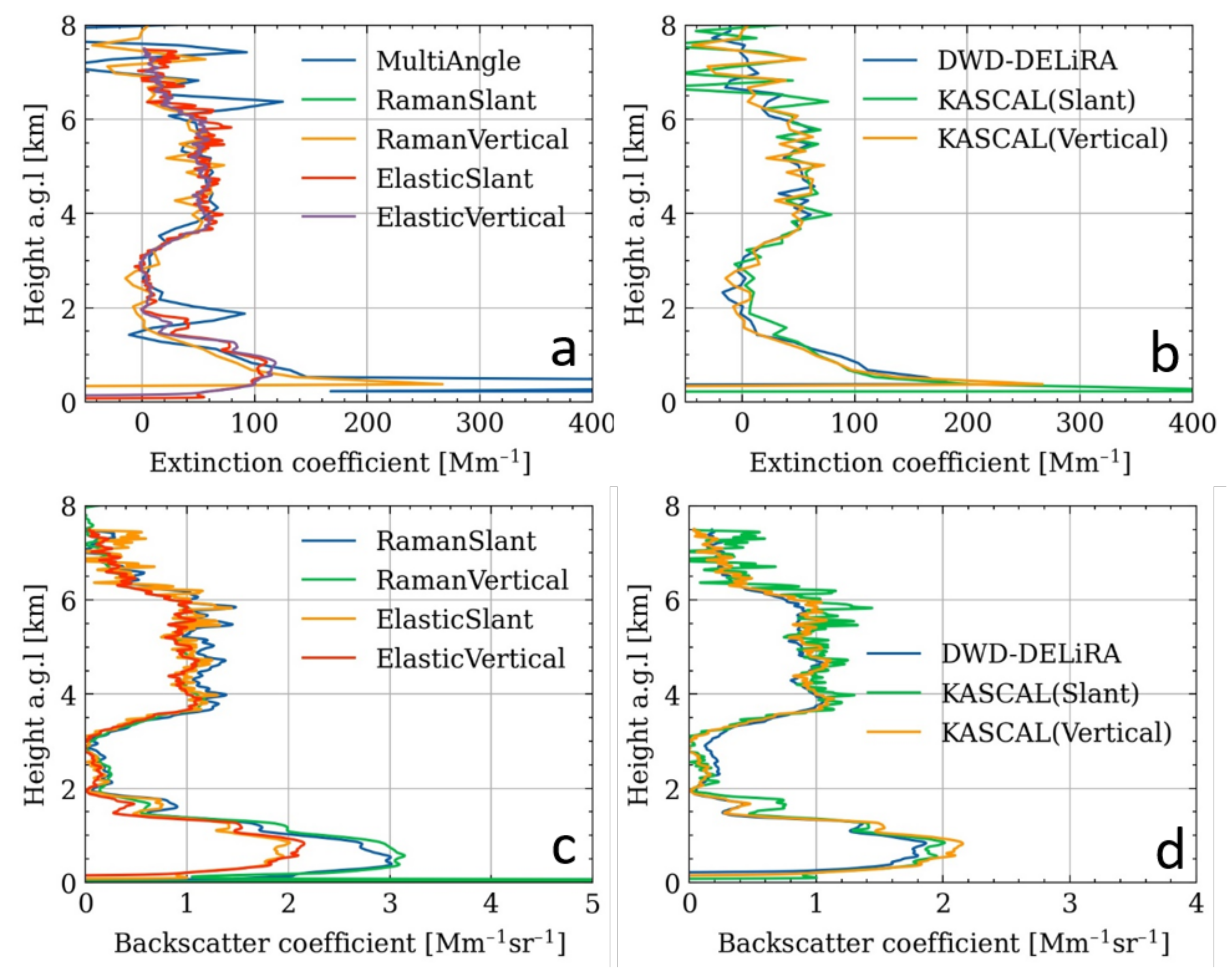
3.1. Application of Two-Angle LiDAR Measurements for a Saharan Dust Case

The method to retrieve LiDAR ratios discussed in the Methods Section was applied for a Saharan dust event from 19:21 to 22:54 (UTC) on 8 April 2018 with the dust layer at an altitude between 2.5 km and 6.0 km. We chose this time period since we had a well-stratified dust layer and also Raman data available. Figure 3 shows backscatter coefficients from vertical and slant LiDAR measurements for different values of assumed LiDAR ratios ranging from 20 sr to 80 sr. Consistent backscatter values for vertical and slant profiles in the dust layer are only available for a LiDAR ratio of 50 sr. This means that a LiDAR ratio of around 50 sr at the Saharan dust layer can be derived from this case, which is a typical value for Saharan dust over Europe [89].
Figure 3a shows that the backscatter coefficients for vertical and slant measurements were consistent for Saharan dust particles (2.5–6.0 km), but inconsistent for boundary layer aerosol particles (below 1 km) when the LiDAR ratio was assumed to be 50 sr. This is because a LiDAR ratio of 50 sr is not suitable for boundary layer aerosol particles at this location [21]. Therefore, we calculated LiDAR ratios based on our Raman signals for boundary layer aerosol particles and the Saharan dust particles. The results are shown in the right panel of Figure 4. The LiDAR ratio for the dust particles was 46 ± 5 sr and for the boundary layer aerosol particles 31 ± 3 sr as the average of both vertical and slant measurements. We parameterised these LiDAR ratios of 46 sr and 31 sr, respectively, as a function of altitude with a single step at 2 km and then used this as the LiDAR ratio for the elastic LiDAR signal retrieval. The results are shown in the left of Figure 4. These backscatter coefficients are consistent for vertical and slant measurements for both dust and boundary layer aerosol. A LiDAR ratio of 31 sr below a 2 km altitude led to much better agreement of the backscatter coefficient profiles from the elastic channel and Raman channel compared to Figure 3c. However, there remain small differences at low altitudes for backscatter coefficients from elastic data for two elevation angles. This inconsistency may be related to an inhomogeneous atmosphere in the boundary layer, as can also be seen in the backscatter coefficients calculated from the Raman data.
The application of this multiangle method for this Saharan dust case proved that this method is useful to retrieve LiDAR ratios from scanning elastic LiDAR measurements. Compared with other methods such as Raman or HSRL LiDAR, the multiangle method provides an applicable solution for both day and night as the elastic LiDAR can obtain reliable measurements for both periods. Furthermore, this method can also be used in multi-wavelength scanning LiDAR systems to determine wavelength-dependent LiDAR ratios.

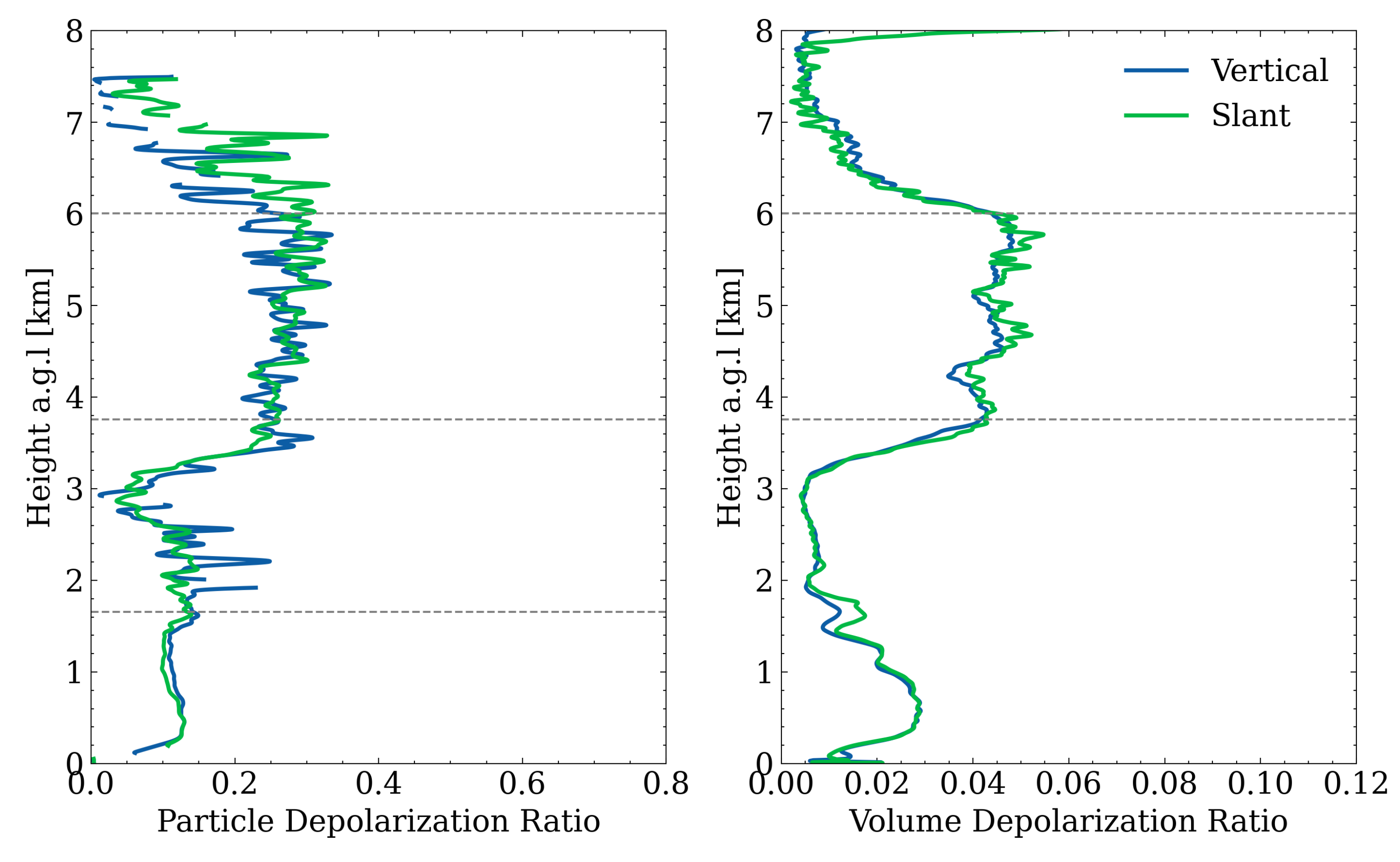
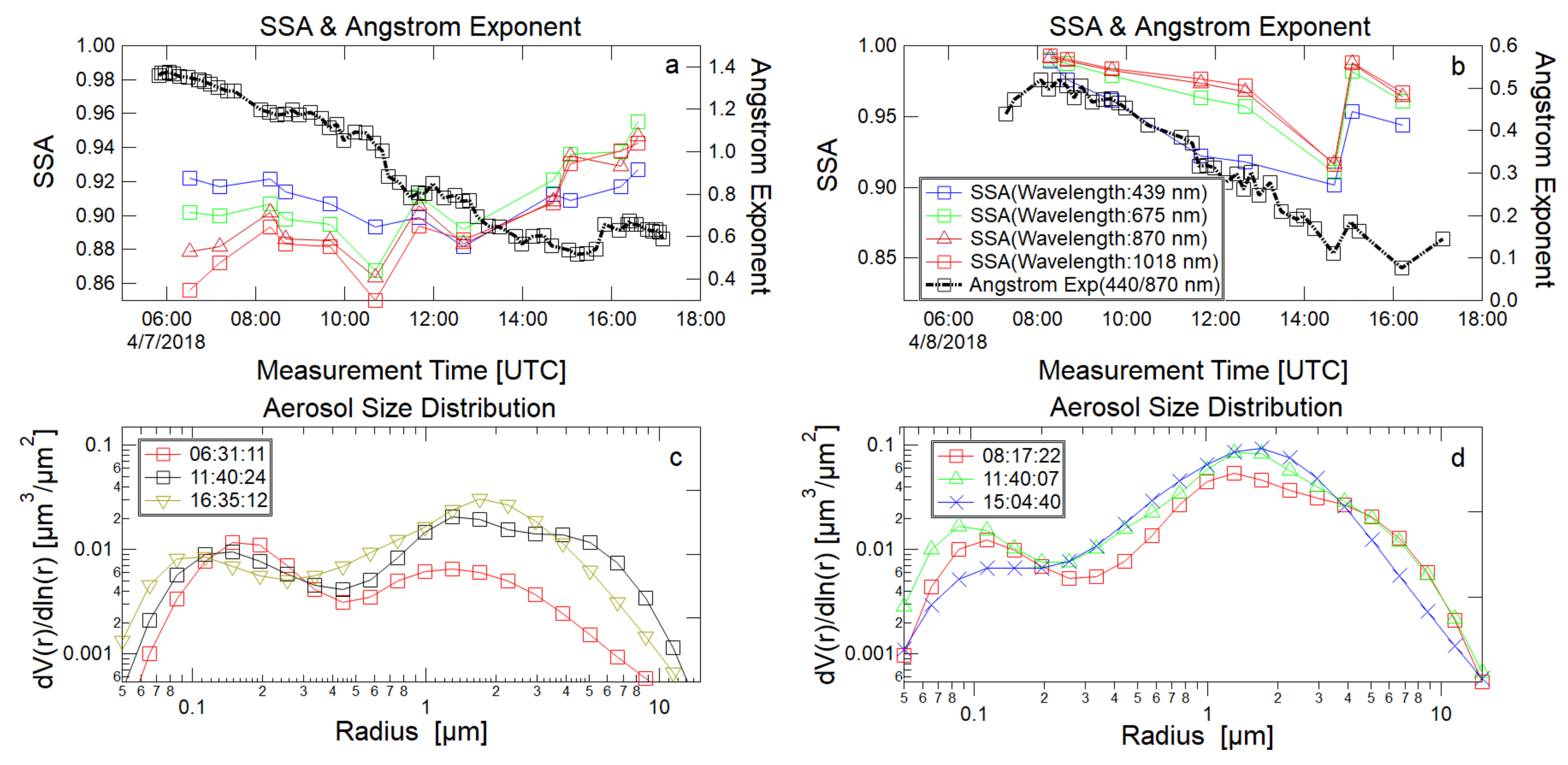
3.2. Characteristic Properties of the Saharan Dust Determined by Remote Sensing

In early April 2018, a far southward-reaching upper-level trough associated with a large low-pressure complex in the western North Atlantic led to a cold front with strong surface winds and dust emission in the Northern Sahara in Morocco and Algeria. The dust was transported northward into the western Mediterranean, where it entered a warm conveyor belt that effectively lifted the dust and transported it towards central Europe. This Saharan dust plume was characterised by the methods described above for nearly three days in April 2018 near the city of Karlsruhe in southwest Germany. The ICON-ART model predicted the arrival of the dust plume and its spatial–temporal evolution as was characterised by LiDAR and sun photometer measurements. Figure 5 shows the corresponding backscatter coefficients from the scanning LiDAR (a), the vertical pointing LiDAR (b), and the ICON-ART model simulation (c), as well as with the linear depolarisation values of the KASCAL (d) for 7–9 April 2018. The scanning LiDAR was operated by performing vertical and slant measurements at 90 and 30 elevation angles alternatingly with integration times for each observation angle of 250 s. The data shown for KASCAL were averaged over two of these measurement periods. The data shown for the DWD-DELiRA were averaged for 30 min. As can be seen in these figures, the plume arrived in Karlsruhe at 11:00 on 7 April (dashed line T1) and lasted about 3 d. Initially, this dust layer showed a maximum of the backscatter at an altitude of 2.5 km, which subsequently also reached lower altitudes. At 12:00 UTC, 8 April, another dust layer between 5.0 km and 11.0 km arrived at the observation station (dashed line T2). Then, the dust layer started sinking and overlapped with the lower dust layer at around 3:00 am of 9 April (dashed line T3). A cloud with a base at 4.5 km appearing at 11:00 (UTC) of 9 April made it difficult to retrieve the backscatter coefficients for the aerosol particles below. Hence, the backscatter coefficients of the LiDAR measurements are not shown for this period. In addition, two periods (C1 and C2) are highlighted for which we performed a more detailed analysis.
All four panels in Figure 5 show a good agreement among dust layer height, dust plume arrival times, and dust plume structures. In particular, ICON-ART predicted the arrival time of the dust plume precisely (±20 min difference with the observations). This indicates that the model reproduced the synoptic scale processes very well, which led to the precise prediction of dust transport. Thus, the general good agreement between LiDAR measurements and ICON-ART partially validated the model’s capabilities to predict dust transport. Please note that this special model run only included desert dust aerosols. Hence, the difference due to boundary layer aerosol particles was expected in this case. Furthermore, there were dust layers predicted by the model for higher altitudes (e.g., a dust plume at around 8 km on 7 April and 8 April), which were not detected by the LiDAR measurements. Potential reasons for the agreement and differences between LiDAR observations and model predictions are discussed in Section 3.3.
During this dust event, the LiDARs used three optical measurement paths (two vertical measurements and one slant measurement with an elevation angle at 30°). The comparison of these three profiles can be used to test different LiDAR retrieval methods and to characterise the properties of the dust plume (e.g., horizontal homogeneity of the dust plume). Figure 6 shows the extinction and backscatter coefficients obtained for different retrieval methods and different optical paths for the measurement time from 19:21 to 22:54 (UTC) of 8 April (period C2 in Figure 5) and averaged over 66 min for scanning LiDAR measurements and 213 min for vertical LiDAR measurements. Please note that the scanning LiDAR measured alternated at two angles (90° and 30°). A LiDAR ratio of 50 sr, which is a typical value observed for Saharan dust [89], was used in the Klett–Fernald method to retrieve the elastic backscatter coefficients and extinction coefficients. Figure 6a,b shows the extinction coefficients from different retrieval methods (elastic, Raman, and multiangle methods) and from different optical paths, respectively. Figure 6c,d shows the backscatter coefficients from different retrieval methods (elastic, Raman, and multiangle methods) and from different optical paths, respectively. The extinction coefficients and backscatter coefficients calculated using the above methods as shown in Figure 6a,c were consistent, but the extinction coefficients calculated from the Raman measurements had larger variations. In addition to the classical methods to retrieve extinction coefficients, we also calculated the extinction coefficients from the elastic channels with a multiangle method, which also agreed with the other methods. The denoising methods can have a substantial impact on the remaining variability of the extinction coefficients retrieved from Raman data. In Figure S1, we provide extinction coefficients retrieved from Raman data for different filters and different filter lengths. In addition, the average extinction coefficients and their standard deviations averaging from 4.0 km to 6.0 km altitude are listed in Table S1. These data show that the mean values of the extinction coefficients for different filter types and filter lengths remained almost constant. In contrast, their uncertainties varied from around 35 Mm 1 to 5 Mm 1 with window lengths from 82.5 m to 1207.5 m for different types of filters. Hence, the Raman extinction coefficients were affected more by the filter window lengths than the filter type, which was in agreement with the observations by Shen and Cao [90]. The backscatter coefficients and extinction coefficients for different optical paths are shown in Figure 6b and Figure 6d, respectively. The consistency of these profiles reflects the high quality of measurements and retrieval algorithms.
A comparison between the active LiDARs and the passive sun photometer can help to understand the properties of the dust aerosol particles employing dust aerosol scattering information from different scattering angles to retrieve dust particles’ microphysical properties. During this dust event, we compared the AOD from DWD-DELiRA measurements and a sun photometer for two continuous days (7–8 April). The AOD from the sun photometer was the AERONET Version 3 level 2.0 product [83], while that of LiDAR measurement was corrected in the following ways. Firstly, as discussed above, two aerosol layers existed with different LiDAR ratios. Hence, we used two different LiDAR ratios at different altitudes to retrieve the backscatter coefficients, which are shown in Figure S2. We used a LiDAR ratio of 50 sr for the upper layer (above 2 km, red line) and 30 sr for the lower layer (below 2 km, green line), typical values for Saharan dust and boundary layer aerosol [89]. Secondly, constant backscatter coefficients were assumed in the LiDAR overlap region, and these constant values were set to be the backscatter coefficients at a range of 255 m (the overlap region of DWD-DELiRA). Finally, the AOD in the far range (e.g., stratosphere) was assumed to be zero. The hourly AODs from the sun photometer, the vertical LiDAR (DWD-DELiRA), and the ICON-ART model are shown in Figure 7. Please note that the model result is discussed in detail in Section 3.3. As the signal-to-noise ratio of the LiDAR is low for KASCAL in the daytime, the AODs were not calculated by this LiDAR. All these three methods showed a similar trend with AODs increasing from around 0.13 to 0.45 during these two days. However, the average AOD retrieved from the LiDAR data for the two days was systematically lower by 0.053 ± 0.031 than that from the sun photometer after wavelength conversion to 340 nm. The AE used for this wavelength conversion was 0.471, which was calculated from the sun photometer data at wavelengths of 340 nm and 380 nm. The average stratospheric AOD for the years 2018-2019 in the Northern Hemisphere was 0.01 at 340 nm [91]. Hence, the averaged AOD measured by the sun photometer was still larger by 0.043 ± 0.031 than the AOD from the LiDAR measurement even considering stratospheric AOD. This bias may be due to an inappropriate assumption of constant backscatter coefficients in the overlap region of the LiDAR. Such an uncertainty of the AOD corresponds to an uncertainty in backscatter coefficients of 5.6 ± 4.1 Mm 1 sr 1 in the overlap region, which is reasonable for typical boundary layer aerosol variations [92,93,94]. On 8 April, clouds led to increased uncertainties in AOD retrievals from the LiDAR measurements and also some data gaps in the sun photometer. Hence, the AOD from LiDAR measurements can be given only for some selected clear sky periods while the sun photometer has still enough valid data points to calculate hourly averages.
For this dust event, vertical and slant volume ( δ v ) and particle ( δ p ) depolarisation ratios were measured by the two different LiDAR systems, and the volume depolarisation ratios for these two elevation angles are shown in Figure 8. No obvious difference between vertical and slant measurements was found for volume depolarisation ratios and particle depolarisation ratios. This may mean that the dust particle had no specific orientation [95,96]. The particle depolarisation ratio of this dust plume was 0.27 ± 0.023, which is very similar to, but slightly larger than the depolarisation ratios determined at 532 nm for Saharan dust particles [13,97]. However, this is still within the combined uncertainty limits. Furthermore, the day-to-day variability of the values given by Freudenthaler et al. [13] ranged from about 0.22 to 0.31.
Figure 9 shows the SSA, AE, and ASD calculated based on the sun photometer measurements on 7 and 8 April. The AE at wavelengths of 440/880 nm decreased from 1.38 to 0.08 during these two days, as shown in Figure 9a,b. This may be related to a smaller wavelength dependence of the AOD, which may be caused by larger particles. Particle size distributions provided by sun photometer retrievals are shown in Figure 9c,d. They indeed showed increasing amounts of larger particles. The maximum column-integrated volume concentration of coarse mode particles increased from around 0.007 μ m 3 / μ m 2 in the early morning of 7 April (before Saharan dust arrival) to 0.093 μ m 3 / μ m 2 in the afternoon of 8 April. The Single Scattering Albedos (SSAs) determined for the wavelengths between 439 nm and 1018 nm ranged between 0.88 and 0.96 and agreed quite well with the data from previous observations (cf. Table S2).

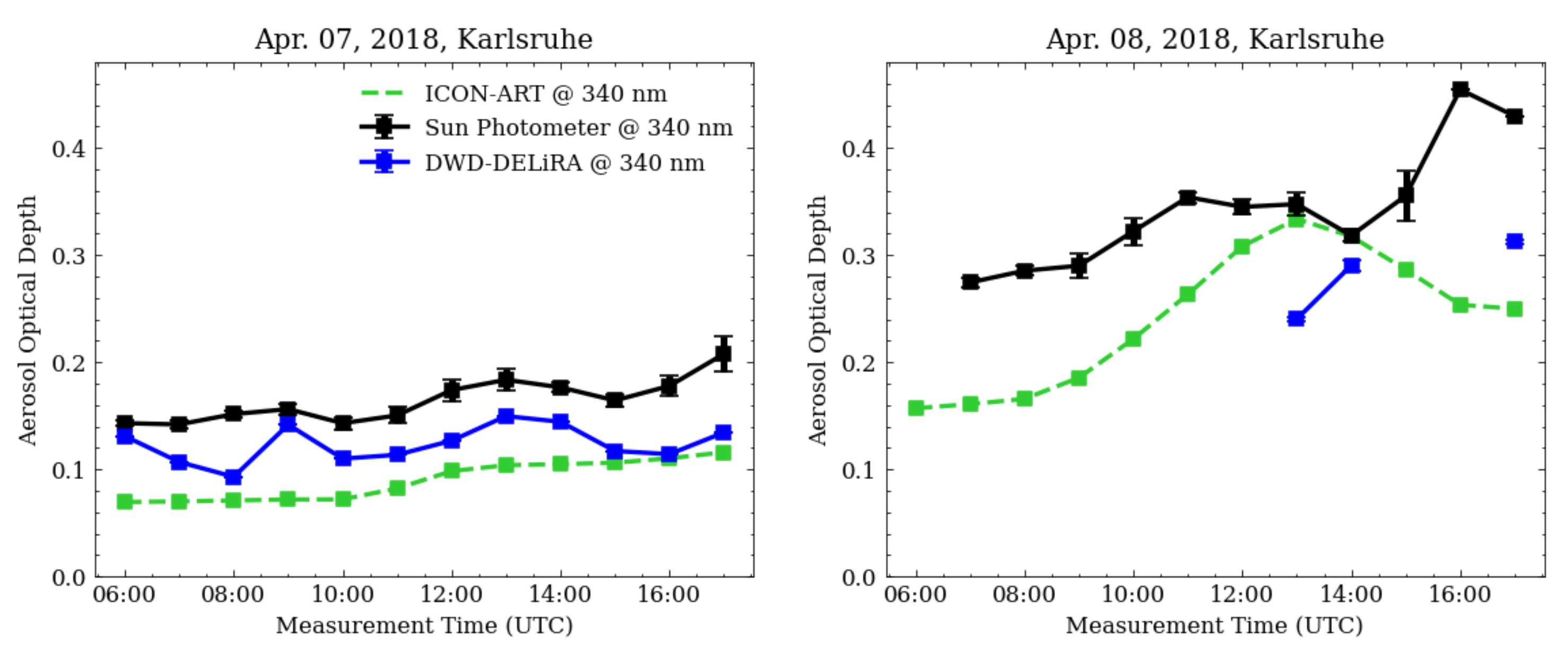
3.3. Model–Observation Comparison

Model simulations and LiDAR observations were used to study the spatial and temporal evolution of a dust plume in this study. The comparison between the model and LiDAR results can be used to evaluate the performance of the model simulation including dust layer height, dust arrival time, dust layer structure, and dust optical parameters. The evolution of the dust plume over Karlsruhe predicted by the ICON-ART model is shown in Panel (c) of Figure 5. According to the model simulation, the dust layer arrived in Karlsruhe at 11:00 of 7 April, and this plume passed over that location for nearly two and a half days. Two dust layers were observed from time 12:00 (UTC) of 8 April to the morning of 9 April, then they merged. A comparison between the model prediction and LiDAR measurement is shown in Panel (b) of Figure 5, where the black contour line is the modelled backscatter coefficient and the contour fill is the LiDAR (DWD-DELiRA) observation. The white line in Panel (b) is the cloud base height from the LiDAR measurements. The dust layer heights (vertical extend) and their peak heights (the heights for the maximum backscatter coefficients) for both the LiDAR measurements and ICON-ART prediction are shown in Figure S3. The criteria for an aloft dust layer are as follows: (i) the δ p value is larger than 0.1 throughout the layer; (ii) the layer thickness exceeds 0.3 km; (iii) the layer base is above the planetary boundary layer [98]. This figure shows a very good agreement in dust layer heights for these two measurements and the ICON-ART prediction. The comparison showed that the dust plume arrival time, layer height, structure, and backscatter coefficients were consistent between the LiDAR measurement and model simulation for this event. Although the LiDAR data showed more details of the dust plume structures, the agreement with the model was quite good considering the relatively coarse spatial resolution used in this model run. On the other hand, in the presence of clouds, aerosol properties cannot be retrieved from LiDAR data. Therefore, a comparison for thin dust layers is not always meaningful. The dust layer height range was based on the dust layer heights shown in Figure S3, which does not include the boundary layer aerosol for LiDAR measurements. All comparisons between LiDAR measurements and ICON-ART model results followed these criteria. A comparison of the vertical backscatter coefficient profiles between LiDARs and ICON-ART model predictions is shown in the right of Figure 5. The backscatter coefficients are given for LiDAR measurements from 15:30 to 16:30 and ICON-ART calculations for 16:00 on 7 April. This figure shows a good agreement in the dust layer vertical extent of the backscatter coefficients from the model calculation for this time period. The comparison between the LiDAR and ICON-ART model showed that the ICON-ART predictions agreed very well with the measurements, although some variability can be observed as well.
Besides, the AODs for three wavelengths from the sun photometer and model calculation are shown in Figure 10. This figure shows that the AODs from the sun photometer and model showed a similar trend. However, the modelled AODs were systematically lower than those from the sun photometer. Figure S4 shows the time series of coarse particle mode AOD for the sun photometer and modelled AOD, which showed that the modelled AOD values agreed well with the coarse mode AOD of the sun photometer at a wavelength of 550 nm. Hence, the reason for underestimating the AOD by the model shown in Figure 10 is partially due to the fact that the modelled AOD only included the Saharan dust plume and the sun photometer also included the boundary layer aerosol. After the arrival of the dust plume, the AOD from model calculation was systematically lower than the sun photometer measurement, and the bias between the model and sun photometer increased with decreasing wavelength towards the ultraviolet (UV) spectral region. In other words, the discrepancy was wavelength dependent with a bigger difference in the UV.
Figure 11 shows the correlation of the backscatter coefficients from LiDAR measurements and ICON-ART simulations for the dust plume, assuming both Non-Spherical (NSP) (left panel) and Spherical (SPH) (right panel) particles. The colour of the scatter points in this figure indicates the normalised density of the backscatter coefficients, which indicates the frequency of the occurrence of these values. These data points were selected for the dust layers shown in Figure S3, which does not include the boundary layer aerosol for the LiDAR measurements. The parameterisations for the NSP and SPH are given in Hoshyaripour et al. [73] and were based on the work by Meng et al. [88]. For the whole dust episode, there was a remarkable agreement between the model simulation and observations, although individual profiles might differ significantly. The regression fitting was performed for both the NSP and SPH data points, which had a normalised density greater than 0.4. The corresponding results of a regression analysis for the NSP showed a slope of 0.9 ± 0.1 and a R 2 of 0.68. This is an excellent result taking into account all uncertainties and assumptions for measurements and model simulations. However, the regression fitting for the SPH had a slope of 2.3 ± 0.3 and an R 2 of 0.68. This means that assuming spherical particles led to overestimated backscatter coefficients. This is confirmed in Figure S5, which shows the backscatter coefficients of two LiDAR measurements and two model simulations using SPH and NSP parameterisations, respectively. This figure shows that the ICON-ART model overestimated the backscatter coefficients at a wavelength of 355 nm by assuming spherical particles to calculate the backscatter coefficients. The mean value and standard derivation of the backscatter coefficient from the LiDAR measurement and ICON-ART simulation are shown in Table S3, which also confirmed that an inappropriate parameterisation would overestimate the predicted backscatter coefficient. The reason for the overestimation was that the spherical particles have larger backscatter coefficients (at 180 ) than non-spherical particles [73,99]. The physical meaning behind this phenomenon is that for spherical particles, surface waves can contribute to the backscatter, hence causing larger backscatter coefficients for spherical particles [100]. The vertical profiles of the backscatter coefficient from two LiDAR measurements and two ICON-ART modes are shown in Figure S6 for two selected periods, indicated as C1 and C2 in Figure 5. Comparing Figure S5 and Figure S6, we found that ICON-ART could predict dust layer structures quite well for most of the time of this event, but also showed substantial differences from the LiDAR measurements, e.g., for the time period C2 (cf. Figure S6 right). The coarse mode AOD of the sun photometer and ICON-ART results for spherical and non-spherical particle models are shown in Figure S4. All AOD values followed a similar trend, but the model results were higher by a factor of 1.25 ± 0.21 for NSP particles and 1.14 ± 0.18 at a wavelength of 550 nm for SPH particles at a wavelength of 550 nm.

4. Conclusions

The objectives of this work were to compare different measurements and retrieval methods including scanning LiDAR measurements and sun photometer data and to demonstrate which aerosol properties can be determined by combining the different measurement techniques. Furthermore, we wanted to understand the quality of the dust plume predictions with the ICON-ART model by comparison with the observations. The evolution and the properties of a Saharan dust plume were characterised for two and a half days combining data from a scanning LiDAR, a vertical LiDAR, and a sun photometer. The comprehensive dataset from different methods could characterise the dust plume in different ways, thus providing additional information for further analysis. The scanning angle LiDAR measurements enabled us to retrieve LiDAR ratios and extinction coefficients independently and during day and night, which were comparable to the Raman-based retrievals. The comparison of extinction and backscatter coefficients for different retrieval methods was used to quantify the uncertainties of the different methods and the impact of different denoising filters on the extinction coefficients from Raman scattering LiDAR signals. The consistency among three different LiDAR laser beam paths reflected the high quality of the measurements, as well as the retrieval algorithms. Vertical and slant volume and particle depolarisation ratio measurements contained information on the shape and partially the orientation of dust particles. The comparison between LiDAR and sun photometer measurements proved useful to study the dust optical properties such as aerosol optical depth and to obtain information about LiDAR parameters such as the LiDAR ratio. Wavelength-dependent optical parameters and the microphysics of dust particles provided by the sun photometer indicated larger particles over the observation station for this dust event. The comparison between LiDAR measurements, the sun photometer, and ICON-ART predictions showed a quite good agreement for the dust arrival time, dust layer height and structure, backscatter coefficients, and AODs. The average AOD from the model was larger by a factor of 1.25 ± 0.21 compared to the sun photometer at a wavelength of 550 nm. The modelled backscatter coefficients for dust showed a correlation with a slope of 0.9 ± 0.1 (R 2 =0.68) for a wavelength of 355 nm with LiDAR observations. However, the model can overestimate the observed backscatter coefficients if assuming spherical particles. The corresponding correlation between the model and LiDAR data showed a slope of 2.3 ± 0.3 (R 2 = 0.74). This demonstrates how crucial it is to use an appropriate parameterisation for the dust particle optics. This has implications for the particle assimilation scheme of the models. Despite the good agreement between model predictions and observations for this Saharan dust plume at one location, we cannot generalise this result. Systematic comparisons for different meteorological conditions and at different locations are needed to substantiate the model validation and to facilitate a potential improvement of the dust processes (emission, transport, removal, and microphysics) and properties (size distribution and optics) in the models.

Supplementary Materials

The following are available online at https://www.mdpi.com/article/10.3390/rs14071693/s1, Figure S1: Extinction coefficients from the Raman signal from vertical and slant measurements with different types of filters and different filter lengths, Figure S2: Elastic backscatter coefficients from vertical LiDAR measurements for different values of altitude-dependent LiDAR ratios with the interval time being 1 h, Figure S3: Time series of dust layer heights and peak heights (the heights for the maximum backscatter coefficients) for both LiDAR measurements and ICON-ART prediction, as well as cloud base heights (green line) measured by LiDAR from 7 to 9 April 2018, Figure S4: AOD from the sun photometer (coarse mode) and ICON-ART for both SPH and NSP particles model simulation on 7 and 8 April for a 1 h temporal resolution. SPH = spherical; NSP = non-spherical, Figure S5: Time series of backscatter coefficients from KASCAL measurements (a) and from DWD-DELiRA measurements with ICON-ART results shown as black contour lines (b), as well as ICON-ART results for SPH particles (c) and as ICON-ART results for NSP particles from 7 to 9 April 2018. Please note that the model data only include the Saharan dust, while the LiDAR data show also other aerosol particles and clouds. The profiles of backscatter coefficients measured by the two LiDARs from 15:30 to 16:30 and predicted by ICON-ART for 16:00 on 7 April 2018 (indicated as C1 in the contour plots) are shown on the right side of this figure. The vertical dashed lines in the contour plots indicate dust arrival (T1), second dust layer appearance (T2), and the two dust layers merging (T3). C1 and C2 represent the time periods used for a more detailed data analysis. SPH = spherical; NSP = non-spherical, Figure S6: Profiles of the backscatter coefficient from KASCAL (both vertical and slant direction), DWD-DELiRA measurements, as well as ICON-ART model simulation for two typical cases indicated as C1 (left) and C2 (right) in Figure 1. SPH = spherical; NSP = non-spherical, Table S1: Averaged extinction coefficients and their standard deviations for different window types and lengths, Table S2: Overview of SSAs measured for Saharan dust, Table S3: Comparison of backscatter coefficients from LiDAR and ICON-ART based on spherical parameterisation (SPH) and non-spherical parameterisation (NSP). Appendix: Mathematical derivation of the multiangle method.

Author Contributions

F.W. and H.S. performed the measurements. G.H., H.V., V.B. and J.F. conducted the model simulations and post-processing of the outputs. H.Z. and F.W. analysed the remote sensing data. H.Z. wrote the manuscript with support from F.W., T.L. and H.S., as well as contributions from all co-authors. All authors have read and agreed to the published version of the manuscript.

Funding

Support by the staff of the Institute of Meteorology and Climate Research, financial support by the project Modular Observation Solutions for Earth Systems (MOSES) of the Helmholtz Association (HGF), and the German Federal Ministry for Economic Affairs and Energy project PerduS (support ID: 0325932B) are gratefully acknowledged. We acknowledge support by the KIT-Publication Fund of the Karlsruhe Institute of Technology.

Institutional Review Board Statement

Not applicable.

Informed Consent Statement

Not applicable.

Data Availability Statement

The LiDAR data are available upon request to the corresponding author. The sun photometer data are available from the AErosol RObotic NETwork (AERONET) data centre at https://AERONET.gsfc.nasa.gov/ (accessed on 8 May 2021). The ICON-ART model simulation results are available upon request from the data originator (DWD; [email protected]).

Conflicts of Interest

The authors declare no conflict of interest.

Abbreviations

The following abbreviations are used in this manuscript:
KASCALKarlsruhe Scanning Aerosol LiDAR
DWD-DELiRADeutscher Wetterdienst-Depolarization Raman LiDAR

References

  1. Stocker, T. Climate Change 2013: The Physical Science Basis: Working Group I Contribution to the Fifth Assessment Report of the Intergovernmental Panel on Climate Change; Cambridge University Press: Cambridge, UK, 2014. [Google Scholar]
  2. Satheesh, S.; Srinivasan, J.; Moorthy, K. Spatial and temporal heterogeneity in aerosol properties and radiative forcing over Bay of Bengal: Sources and role of aerosol transport. J. Geophys. Res. Atmos. 2006, 111. [Google Scholar] [CrossRef] [Green Version]
  3. Ansmann, A.; Tesche, M.; Althausen, D.; Müller, D.; Seifert, P.; Freudenthaler, V.; Heese, B.; Wiegner, M.; Pisani, G.; Knippertz, P.; et al. Influence of Saharan dust on cloud glaciation in southern Morocco during the Saharan Mineral Dust Experiment. J. Geophys. Res. Atmos. 2008, 113. [Google Scholar] [CrossRef]
  4. Su, J.; Huang, J.; Fu, Q.; Minnis, P.; Ge, J.; Bi, J. Estimation of Asian dust aerosol effect on cloud radiation forcing using Fu-Liou radiative model and CERES measurements. Atmos. Chem. Phys. 2008, 8, 2763–2771. [Google Scholar]
  5. DeMott, P.J.; Prenni, A.J.; McMeeking, G.R.; Sullivan, R.C.; Petters, M.D.; Tobo, Y.; Niemand, M.; Möhler, O.; Snider, J.R.; Wang, Z.; et al. Integrating laboratory and field data to quantify the immersion freezing ice nucleation activity of mineral dust particles. Atmos. Chem. Phys. 2015, 15, 393–409. [Google Scholar] [CrossRef] [Green Version]
  6. Möhler, O.; Adams, M.; Lacher, L.; Vogel, F.; Nadolny, J.; Ullrich, R.; Boffo, C.; Pfeuffer, T.; Hobl, A.; Weiß, M.; et al. The Portable Ice Nucleation Experiment (PINE): A new online instrument for laboratory studies and automated long-term field observations of ice-nucleating particles. Atmos. Meas. Tech. 2021, 14, 1143–1166. [Google Scholar] [CrossRef]
  7. Brunner, C.; Brem, B.T.; Collaud Coen, M.; Conen, F.; Hervo, M.; Henne, S.; Steinbacher, M.; Gysel-Beer, M.; Kanji, Z.A. The contribution of Saharan dust to the ice-nucleating particle concentrations at the High Altitude Station Jungfraujoch (3580 m a.s.l.), Switzerland. Atmos. Chem. Phys. 2021, 21, 18029–18053. [Google Scholar] [CrossRef]
  8. Niemand, M.; Möhler, O.; Vogel, B.; Vogel, H.; Hoose, C.; Connolly, P.; Klein, H.; Bingemer, H.; DeMott, P.; Skrotzki, J.; et al. A particle-surface-area-based parameterization of immersion freezing on desert dust particles. J. Atmos. Sci. 2012, 69, 3077–3092. [Google Scholar] [CrossRef]
  9. Min, Q.L.; Li, R.; Lin, B.; Joseph, E.; Wang, S.; Hu, Y.; Morris, V.; Chang, F. Evidence of mineral dust altering cloud microphysics and precipitation. Atmos. Chem. Phys. 2009, 9, 3223–3231. [Google Scholar] [CrossRef] [Green Version]
  10. Karydis, V.A.; Tsimpidi, A.P.; Bacer, S.; Pozzer, A.; Nenes, A.; Lelieveld, J. Global impact of mineral dust on cloud droplet number concentration. Atmos. Chem. Phys. 2017, 17, 5601–5621. [Google Scholar] [CrossRef] [Green Version]
  11. Meloni, D.; Di Sarra, A.; Di Iorio, T.; Fiocco, G. Influence of the vertical profile of Saharan dust on the visible direct radiative forcing. J. Quant. Spectrosc. Radiat. Transf. 2005, 93, 397–413. [Google Scholar] [CrossRef]
  12. Ma, P.L.; Rasch, P.J.; Chepfer, H.; Winker, D.M.; Ghan, S.J. Observational constraint on cloud susceptibility weakened by aerosol retrieval limitations. Nat. Commun 2018, 9, 1–10. [Google Scholar] [CrossRef]
  13. Freudenthaler, V.; Esselborn, M.; Wiegner, M.; Heese, B.; Tesche, M.; Ansmann, A.; Müller, D.; Althausen, D.; Wirth, M.; Fix, A.; et al. Depolarization ratio profiling at several wavelengths in pure Saharan dust during SAMUM 2006. Tellus B Chem. Phys. Meteorol. 2009, 61, 165–179. [Google Scholar] [CrossRef] [Green Version]
  14. Kanitz, T.; Engelmann, R.; Heinold, B.; Baars, H.; Skupin, A.; Ansmann, A. Tracking the Saharan Air Layer with shipborne LiDAR across the tropical Atlantic. Geophys. Res. Lett. 2014, 41, 1044–1050. [Google Scholar] [CrossRef]
  15. Soupiona, O.; Papayannis, A.; Kokkalis, P.; Foskinis, R.; Sánchez Hernández, G.; Ortiz-Amezcua, P.; Mylonaki, M.; Papanikolaou, C.A.; Papagiannopoulos, N.; Samaras, S.; et al. EARLINET observations of Saharan dust intrusions over the northern Mediterranean region (2014–2017): Properties and impact on radiative forcing. Atmos. Chem. Phys. 2020, 20, 15147–15166. [Google Scholar] [CrossRef]
  16. Marinou, E.; Amiridis, V.; Binietoglou, I.; Tsikerdekis, A.; Solomos, S.; Proestakis, E.; Konsta, D.; Papagiannopoulos, N.; Tsekeri, A.; Vlastou, G.; et al. Three-dimensional evolution of Saharan dust transport towards Europe based on a 9-year EARLINET-optimized CALIPSO dataset. Atmos. Chem. Phys. 2017, 17, 5893–5919. [Google Scholar] [CrossRef] [Green Version]
  17. Akritidis, D.; Katragkou, E.; Georgoulias, A.K.; Zanis, P.; Kartsios, S.; Flemming, J.; Inness, A.; Douros, J.; Eskes, H. A complex aerosol transport event over Europe during the 2017 Storm Ophelia in CAMS forecast systems: Analysis and evaluation. Atmos. Chem. Phys. 2020, 20, 13557–13578. [Google Scholar] [CrossRef]
  18. Osborne, M.; Malavelle, F.F.; Adam, M.; Buxmann, J.; Sugier, J.; Marenco, F.; Haywood, J. Saharan dust and biomass burning aerosols during ex-hurricane Ophelia: Observations from the new UK LiDAR and sun-photometer network. Atmos. Chem. Phys. 2019, 19, 3557–3578. [Google Scholar] [CrossRef] [Green Version]
  19. Mona, L.; Papagiannopoulos, N.; Basart, S.; Baldasano, J.; Binietoglou, I.; Cornacchia, C.; Pappalardo, G. EARLINET dust observations vs. BSC-DREAM8b modelled profiles: 12-year-long systematic comparison at Potenza, Italy. Atmos. Chem. Phys. 2014, 14, 8781–8793. [Google Scholar] [CrossRef] [Green Version]
  20. Müller, D.; Weinzierl, B.; Petzold, A.; Kandler, K.; Ansmann, A.; Müller, T.; Tesche, M.; Freudenthaler, V.; Esselborn, M.; Heese, B.; et al. Mineral dust observed with AERONET Sun photometer, Raman LiDAR, and in situ instruments during SAMUM 2006: Shape-independent particle properties. J. Geophys. Res. Atmos. 2010, 115. [Google Scholar] [CrossRef] [Green Version]
  21. Groß, S.; Tesche, M.; Freudenthaler, V.; Toledano, C.; Wiegner, M.; Ansmann, A.; Althausen, D.; Seefeldner, M. Characterization of Saharan dust, marine aerosols and mixtures of biomass-burning aerosols and dust by means of multi-wavelength depolarization and Raman LiDAR measurements during SAMUM 2. Tellus B Chem. Phys. Meteorol. 2011, 63, 706–724. [Google Scholar] [CrossRef]
  22. Heintzenberg, J. The SAMUM-1 experiment over Southern Morocco: Overview and introduction. Tellus B Chem. Phys. Meteorol. 2009, 61, 2–11. [Google Scholar] [CrossRef]
  23. Petzold, A.; Rasp, K.; Weinzierl, B.; Esselborn, M.; Hamburger, T.; Doernbrack, A.; Kandler, K.; SchuüTZ, L.; Knippertz, P.; Fiebig, M.; et al. Saharan dust absorption and refractive index from aircraft-based observations during SAMUM 2006. Tellus B Chem. Phys. Meteorol. 2009, 61, 118–130. [Google Scholar] [CrossRef] [Green Version]
  24. Kandler, K.; Schütz, L.; Deutscher, C.; Ebert, M.; Hofmann, H.; Jäckel, S.; Jaenicke, R.; Knippertz, P.; Lieke, K.; Massling, A.; et al. Size distribution, mass concentration, chemical and mineralogical composition and derived optical parameters of the boundary layer aerosol at Tinfou, Morocco, during SAMUM 2006. Tellus B Chem. Phys. Meteorol. 2009, 61, 32–50. [Google Scholar] [CrossRef] [Green Version]
  25. Weinzierl, B.; Petzold, A.; Esselborn, M.; Wirth, M.; Rasp, K.; Kandler, K.; Schuetz, L.; Koepke, P.; Fiebig, M. Airborne measurements of dust layer properties, particle size distribution and mixing state of Saharan dust during SAMUM 2006. Tellus B Chem. Phys. Meteorol. 2009, 61, 96–117. [Google Scholar] [CrossRef] [Green Version]
  26. Kandler, K.; Lieke, K.; Benker, N.; Emmel, C.; Küpper, M.; Müller-Ebert, D.; Ebert, M.; Scheuvens, D.; Schladitz, A.; Schütz, L.; et al. Electron microscopy of particles collected at Praia, Cape Verde, during the Saharan Mineral Dust Experiment: Particle chemistry, shape, mixing state and complex refractive index. Tellus B Chem. Phys. Meteorol. 2011, 63, 475–496. [Google Scholar] [CrossRef]
  27. Ansmann, A.; Petzold, A.; Kandler, K.; Tegen, I.; Wendisch, M.; Mueller, D.; Weinzierl, B.; Mueller, T.; Heintzenberg, J. Saharan Mineral Dust Experiments SAMUM–1 and SAMUM–2: What have we learned? Tellus B Chem. Phys. Meteorol. 2011, 63, 403–429. [Google Scholar] [CrossRef] [Green Version]
  28. Schladitz, A.; Müller, T.; Nordmann, S.; Tesche, M.; Gross, S.; Freudenthaler, V.; Gasteiger, J.; Wiedensohler, A. In situ aerosol characterization at Cape Verde: Part 2: Parametrization of relative humidity-and wavelength-dependent aerosol optical properties. Tellus B Chem. Phys. Meteorol. 2011, 63, 549–572. [Google Scholar] [CrossRef] [Green Version]
  29. Weinzierl, B.; Sauer, D.; Esselborn, M.; Petzold, A.; Veira, A.; Rose, M.; Mund, S.; Wirth, M.; Ansmann, A.; Tesche, M.; et al. Microphysical and optical properties of dust and tropical biomass burning aerosol layers in the Cape Verde region—An overview of the airborne in situ and LiDAR measurements during SAMUM-2. Tellus B Chem. Phys. Meteorol. 2011, 63, 589–618. [Google Scholar] [CrossRef] [Green Version]
  30. Haarig, M.; Walser, A.; Ansmann, A.; Dollner, M.; Althausen, D.; Sauer, D.; Farrell, D.; Weinzierl, B. Profiles of cloud condensation nuclei, dust mass concentration, and ice-nucleating-particle-relevant aerosol properties in the Saharan Air Layer over Barbados from polarization LiDAR and airborne in situ measurements. Atmos. Chem. Phys. 2019, 19, 13773–13788. [Google Scholar] [CrossRef] [Green Version]
  31. Papayannis, A.; Mamouri, R.E.; Amiridis, V.; Remoundaki, E.; Tsaknakis, G.; Kokkalis, P.; Veselovskii, I.; Kolgotin, A.; Nenes, A.; Fountoukis, C. Optical-microphysical properties of Saharan dust aerosols and composition relationship using a multi-wavelength Raman LiDAR, in situ sensors and modelling: A case study analysis. Atmos. Chem. Phys. 2012, 12, 4011–4032. [Google Scholar] [CrossRef] [Green Version]
  32. Perrone, M.R.; Barnaba, F.; De Tomasi, F.; Gobbi, G.P.; Tafuro, A.M. Imaginary refractive-index effects on desert-aerosol extinction versus backscatter relationships at 351 nm: Numerical computations and comparison with Raman LiDAR measurements. Appl. Opt. 2004, 43, 5531–5541. [Google Scholar] [CrossRef] [PubMed]
  33. Killinger, D.K.; Menyuk, N. Laser remote sensing of the atmosphere. Science 1987, 235, 37–45. [Google Scholar] [CrossRef] [PubMed]
  34. Fernald, F.G. Analysis of atmospheric LiDAR observations: Some comments. Appl. Opt. 1984, 23, 652–653. [Google Scholar] [CrossRef] [PubMed]
  35. Klett, J.D. LiDAR inversion with variable backscatter/extinction ratios. Appl. Opt. 1985, 24, 1638–1643. [Google Scholar] [CrossRef] [PubMed]
  36. Haarig, M.; Ansmann, A.; Baars, H.; Jimenez, C.; Veselovskii, I.; Engelmann, R.; Althausen, D. Depolarization and LiDAR ratios at 355, 532, and 1064 nm and microphysical properties of aged tropospheric and stratospheric Canadian wildfire smoke. Atmos. Chem. Phys. 2018, 18, 11847–11861. [Google Scholar] [CrossRef] [Green Version]
  37. Haarig, M.; Ansmann, A.; Engelmann, R.; Baars, H.; Toledano, C.; Torres, B.; Althausen, D.; Radenz, M.; Wandinger, U. First triple-wavelength LiDAR observations of depolarization and extinction-to-backscatter ratios of Saharan dust. Atmos. Chem. Phys. 2022, 22, 355–369. [Google Scholar] [CrossRef]
  38. Lei, L.; Berkoff, T.A.; Gronoff, G.P.; Su, J.; Nehrir, A.R.; Wu, Y.; Moshary, F.; Kuang, S. Retrieval of UVB aerosol extinction profiles from the ground-based Langley Mobile Ozone LiDAR (LMOL) system. Atmos. Meas. Tech. Discuss. 2021, 2021, 1–22. [Google Scholar] [CrossRef]
  39. Wandinger, U. Raman LiDAR. In LiDAR; Springer: Berlin/Heidelberg, Germany, 2005; pp. 241–271. [Google Scholar]
  40. Liu, Z.; Matsui, I.; Sugimoto, N. High-spectral-resolution LiDAR using an iodine absorption filter for atmospheric measurements. Opt. Eng. 1999, 38, 1661–1670. [Google Scholar] [CrossRef]
  41. Piironen, P.; Eloranta, E. Demonstration of a high-spectral-resolution LiDAR based on an iodine absorption filter. Opt. Lett. 1994, 19, 234–236. [Google Scholar]
  42. Schillinger, M.; Morancais, D.; Fabre, F.; Culoma, A.J. ALADIN: The LiDAR instrument for the AEOLUS mission. In Sensors, Systems, and Next-Generation Satellites VI; Fujisada, H., Lurie, J.B., Aten, M.L., Weber, K., Lurie, J.B., Aten, M.L., Weber, K., Eds.; International Society for Optics and Photonics, SPIE: Bellingham, WA, USA, 2003; Volume 4881, pp. 40–51. [Google Scholar]
  43. Chen, W.N.; Chen, Y.W.; Chou, C.C.; Chang, S.Y.; Lin, P.H.; Chen, J.P. Columnar optical properties of tropospheric aerosol by combined LiDAR and sun photometer measurements at Taipei, Taiwan. Atmos. Environ. 2009, 43, 2700–2708. [Google Scholar] [CrossRef]
  44. Wang, J.; Liu, W.; Liu, C.; Zhang, T.; Liu, J.; Chen, Z.; Xiang, Y.; Meng, X. The determination of aerosol distribution by a no-blind-zone scanning LiDAR. Remote Sens. 2020, 12, 626. [Google Scholar] [CrossRef] [Green Version]
  45. Behrendt, A.; Pal, S.; Wulfmeyer, V.; Lammel, G. A novel approach for the characterization of transport and optical properties of aerosol particles near sources–Part I: Measurement of particle backscatter coefficient maps with a scanning UV LiDAR. Atmos. Environ. 2011, 45, 2795–2802. [Google Scholar] [CrossRef]
  46. Fortich, A.D.; Dominguez, V.; Wu, Y.; Gross, B.; Moshary, F. Observations of Aerosol Spatial Distribution and Emissions in New York City Using a Scanning Micro Pulse LiDAR. In EPJ Web of Conferences; EDP Sciences: Hefei, China, 2020; Volume 237, p. 03020. [Google Scholar]
  47. Ma, X.; Wang, C.; Han, G.; Ma, Y.; Li, S.; Gong, W.; Chen, J. Regional atmospheric aerosol pollution detection based on LiDAR remote sensing. Remote Sens. 2019, 11, 2339. [Google Scholar]
  48. Kokhanenko, G.P.; Balin, Y.S.; Klemasheva, M.G.; Nasonov, S.V.; Novoselov, M.M.; Penner, I.E.; Samoilova, S.V. Scanning polarization LiDAR LOSA-M3: Opportunity for research of crystalline particle orientation in the ice clouds. Atmos. Meas. Tech. 2020, 13, 1113–1127. [Google Scholar] [CrossRef] [Green Version]
  49. Adam, M. Vertical versus scanning LiDAR measurements in a horizontally homogeneous atmosphere. Appl. Opt. 2012, 51, 4491–4500. [Google Scholar] [CrossRef]
  50. Gutkowicz-Krusin, D. Multiangle LiDAR performance in the presence of horizontal inhomogeneities in atmospheric extinction and scattering. Appl. Opt. 1993, 32, 3266–3272. [Google Scholar] [CrossRef]
  51. Kovalev, V.; Wold, C.; Petkov, A.; Hao, W.M. Modified technique for processing multiangle LiDAR data measured in clear and moderately polluted atmospheres. Appl. Opt. 2011, 50, 4957–4966. [Google Scholar] [CrossRef]
  52. Kovalev, V.; Wold, C.; Petkov, A.; Hao, W.M. Direct multiangle solution for poorly stratified atmospheres. Appl. Opt. 2012, 51, 6139–6146. [Google Scholar] [CrossRef]
  53. Kovalev, V.; Wold, C.; Petkov, A.; Hao, W.M. Backscatter near-end solution in processing of scanning LiDAR data. Appl. Opt. 2015, 54, 7335–7341. [Google Scholar] [CrossRef] [PubMed]
  54. Holben, B.N.; Eck, T.F.; Slutsker, I.; Tanre, D.; Buis, J.; Setzer, A.; Vermote, E.; Reagan, J.A.; Kaufman, Y.; Nakajima, T.; et al. AERONET—A federated instrument network and data archive for aerosol characterization. Remote Sens. Environ. 1998, 66, 1–16. [Google Scholar] [CrossRef]
  55. Holben, B.N.; Tanre, D.; Smirnov, A.; Eck, T.; Slutsker, I.; Abuhassan, N.; Newcomb, W.; Schafer, J.; Chatenet, B.; Lavenu, F.; et al. An emerging ground-based aerosol climatology: Aerosol optical depth from AERONET. J. Geophys. Res. Atmos. 2001, 106, 12067–12097. [Google Scholar] [CrossRef]
  56. Pozzoli, L.; Bey, I.; Rast, S.; Schultz, M.; Stier, P.; Feichter, J. Trace gas and aerosol interactions in the fully coupled model of aerosol-chemistry-climate ECHAM5-HAMMOZ: 1. Model description and insights from the spring 2001 TRACE-P experiment. J. Geophys. Res. Atmos. 2008, 113. [Google Scholar] [CrossRef] [Green Version]
  57. Pozzoli, L.; Bey, I.; Rast, S.; Schultz, M.; Stier, P.; Feichter, J. Trace gas and aerosol interactions in the fully coupled model of aerosol-chemistry-climate ECHAM5-HAMMOZ: 2. Impact of heterogeneous chemistry on the global aerosol distributions. J. Geophys. Res. Atmos. 2008, 113. [Google Scholar] [CrossRef] [Green Version]
  58. Roeckner, E.; Brokopf, R.; Esch, M.; Giorgetta, M.; Hagemann, S.; Kornblueh, L.; Manzini, E.; Schlese, U.; Schulzweida, U. Sensitivity of simulated climate to horizontal and vertical resolution in the ECHAM5 atmosphere model. J. Clim. 2006, 19, 3771–3791. [Google Scholar] [CrossRef]
  59. Jöckel, P.; Tost, H.; Pozzer, A.; Brühl, C.; Buchholz, J.; Ganzeveld, L.; Hoor, P.; Kerkweg, A.; Lawrence, M.; Sander, R.; et al. The atmospheric chemistry general circulation model ECHAM5/MESSy1: Consistent simulation of ozone from the surface to the mesosphere. Atmos. Chem. Phys. 2006, 6, 5067–5104. [Google Scholar] [CrossRef] [Green Version]
  60. Jöckel, P.; Kerkweg, A.; Pozzer, A.; Sander, R.; Tost, H.; Riede, H.; Baumgaertner, A.; Gromov, S.; Kern, B. Development cycle 2 of the modular earth submodel system (MESSy2). Geosci. Model Dev. 2010, 3, 717–752. [Google Scholar] [CrossRef] [Green Version]
  61. Kunz, A.; Pan, L.; Konopka, P.; Kinnison, D.; Tilmes, S. Chemical and dynamical discontinuity at the extratropical tropopause based on START08 and WACCM analyses. J. Geophys. Res. Atmos. 2011, 116. [Google Scholar] [CrossRef] [Green Version]
  62. Smith, A.K.; Garcia, R.R.; Marsh, D.R.; Richter, J.H. WACCM simulations of the mean circulation and trace species transport in the winter mesosphere. J. Geophys. Res. Atmos. 2011, 116. [Google Scholar] [CrossRef]
  63. Chapman, E.; Gustafson, W.; Easter, R.; Barnard, J.; Ghan, S.; Pekour, M.; Fast, J. Coupling aerosol-cloud-radiative processes in the WRF-Chem model: Investigating the radiative impact of elevated point sources. Atmos. Chem. Phys. Discuss 2008, 8, 14–765. [Google Scholar] [CrossRef] [Green Version]
  64. Vogel, H.; Förstner, J.; Vogel, B.; Hanisch, T.; Mühr, B.; Schättler, U.; Schad, T. Time-lagged ensemble simulations of the dispersion of the Eyjafjallajökull plume over Europe with COSMO-ART. Atmos. Chem. Phys. 2014, 14, 7837–7845. [Google Scholar] [CrossRef] [Green Version]
  65. Rieger, D.; Steiner, A.; Bachmann, V.; Gasch, P.; Förstner, J.; Deetz, K.; Vogel, B.; Vogel, H. Impact of the 4 April 2014 Saharan dust outbreak on the photovoltaic power generation in Germany. Atmos. Chem. Phys. 2017, 17, 13391–13415. [Google Scholar] [CrossRef] [Green Version]
  66. Weimer, M.; Schröter, J.; Eckstein, J.; Deetz, K.; Neumaier, M.; Fischbeck, G.; Hu, L.; Millet, D.B.; Rieger, D.; Vogel, H.; et al. An emission module for ICON-ART 2.0: Implementation and simulations of acetone. Geosci. Model Dev. 2017, 10, 2471–2494. [Google Scholar] [CrossRef] [Green Version]
  67. Tegen, I.; Fung, I. Modeling of mineral dust in the atmosphere: Sources, transport, and optical thickness. J. Geophys. Res. Atmos. 1994, 99, 22897–22914. [Google Scholar] [CrossRef]
  68. O’Sullivan, D.; Marenco, F.; Ryder, C.L.; Pradhan, Y.; Kipling, Z.; Johnson, B.; Benedetti, A.; Brooks, M.; McGill, M.; Yorks, J.; et al. Models transport Saharan dust too low in the atmosphere: A comparison of the MetUM and CAMS forecasts with observations. Atmos. Chem. Phys. 2020, 20, 12955–12982. [Google Scholar] [CrossRef]
  69. Kang, J.Y.; Yoon, S.C.; Shao, Y.; Kim, S.W. Comparison of vertical dust flux by implementing three dust emission schemes in WRF/Chem. J. Geophys. Res. Atmos. 2011, 116. [Google Scholar] [CrossRef] [Green Version]
  70. Gläser, G.; Kerkweg, A.; Wernli, H. The Mineral Dust Cycle in EMAC 2.40: Sensitivity to the spectral resolution and the dust emission scheme. Atmos. Chem. Phys. 2012, 12, 1611–1627. [Google Scholar] [CrossRef] [Green Version]
  71. Deetz, K.; Klose, M.; Kirchner, I.; Cubasch, U. Numerical simulation of a dust event in northeastern Germany with a new dust emission scheme in COSMO-ART. Atmos. Environ. 2016, 126, 87–97. [Google Scholar] [CrossRef]
  72. Gasch, P.; Rieger, D.; Walter, C.; Khain, P.; Levi, Y.; Knippertz, P.; Vogel, B. Revealing the meteorological drivers of the September 2015 severe dust event in the Eastern Mediterranean. Atmos. Chem. Phys. 2017, 17, 13573–13604. [Google Scholar] [CrossRef] [Green Version]
  73. Hoshyaripour, G.; Bachmann, V.; Förstner, J.; Steiner, A.; Vogel, H.; Wagner, F.; Walter, C.; Vogel, B. Effects of Particle Nonsphericity on Dust Optical Properties in a Forecast System: Implications for Model-Observation Comparison. J. Geophys. Res. Atmos. 2019, 124, 7164–7178. [Google Scholar] [CrossRef]
  74. Forecast Comparison—WMO SDS-WAS. Available online: https://sds-was.aemet.es/forecast-products/dust-forecasts/forecast-comparison (accessed on 22 September 2021).
  75. 3d scanning LIDAR—Raymetrics. Available online: https://www.raymetrics.com/product/3d-scanning-LIDAR (accessed on 14 January 2022).
  76. Avdikos, G. Powerful Raman LiDAR systems for atmospheric analysis and high-energy physics experiments. In EPJ Web of Conferences; EDP Sciences: Padua, Italy, 2015; Volume 89, p. 04003. [Google Scholar]
  77. Freudenthaler, V. About the effects of polarising optics on LiDAR signals and the Δ90 calibration. Atmos. Chem. Phys. 2016, 9, 4181–4255. [Google Scholar] [CrossRef] [Green Version]
  78. Mattis, I.; D’Amico, G.; Baars, H.; Amodeo, A.; Madonna, F.; Iarlori, M. EARLINET Single Calculus Chain–technical–Part 2: Calculation of optical products. Atmos. Meas. Tech. 2016, 9, 3009–3029. [Google Scholar] [CrossRef] [Green Version]
  79. Rocadenbosch, F.; Reba, M.N.M.; Sicard, M.; Comerón, A. Practical analytical backscatter error bars for elastic one-component LiDAR inversion algorithm. Appl. Opt. 2010, 49, 3380–3393. [Google Scholar] [CrossRef] [PubMed]
  80. Ansmann, A.; Wandinger, U.; Riebesell, M.; Weitkamp, C.; Michaelis, W. Independent measurement of extinction and backscatter profiles in cirrus clouds by using a combined Raman elastic-backscatter LiDAR. Appl. Opt. 1992, 31, 7113–7131. [Google Scholar] [CrossRef] [PubMed]
  81. Behrendt, A.; Nakamura, T. Calculation of the calibration constant of polarization LiDAR and its dependency on atmospheric temperature. Opt. Express 2002, 10, 805–817. [Google Scholar] [CrossRef]
  82. Vermeulen, A.; Devaux, C.; Herman, M. Retrieval of the scattering and microphysical properties of aerosols from ground-based optical measurements including polarization. I. Method. Appl. Opt. 2000, 39, 6207–6220. [Google Scholar] [CrossRef]
  83. Sinyuk, A.; Holben, B.N.; Eck, T.F.; Giles, D.M.; Slutsker, I.; Korkin, S.; Schafer, J.S.; Smirnov, A.; Sorokin, M.; Lyapustin, A. The AERONET Version 3 aerosol retrieval algorithm, associated uncertainties and comparisons to Version 2. Atmos. Meas. Tech. 2020, 13, 3375–3411. [Google Scholar] [CrossRef]
  84. Dubovik, O.; King, M.D. A flexible inversion algorithm for retrieval of aerosol optical properties from Sun and sky radiance measurements. J. Geophys. Res. Atmos. 2000, 105, 20673–20696. [Google Scholar] [CrossRef] [Green Version]
  85. Giles, D.M.; Sinyuk, A.; Sorokin, M.G.; Schafer, J.S.; Smirnov, A.; Slutsker, I.; Eck, T.F.; Holben, B.N.; Lewis, J.R.; Campbell, J.R.; et al. Advancements in the Aerosol Robotic Network (AERONET) Version 3 database – automated near-real-time quality control algorithm with improved cloud screening for Sun photometer aerosol optical depth (AOD) measurements. Atmos. Meas. Tech. 2019, 12, 169–209. [Google Scholar] [CrossRef] [Green Version]
  86. Zängl, G.; Reinert, D.; Rípodas, P.; Baldauf, M. The ICON (ICOsahedral Non-hydrostatic) modelling framework of DWD and MPI-M: Description of the non-hydrostatic dynamical core. Q. J. R. Meteorol. Soc. 2015, 141, 563–579. [Google Scholar] [CrossRef]
  87. Vogel, B.; Hoose, C.; Vogel, H.; Kottmeier, C. A model of dust transport applied to the Dead Sea area. Meteorol. Z. 2006, 15, 611–624. [Google Scholar] [CrossRef]
  88. Meng, Z.; Yang, P.; Kattawar, G.W.; Bi, L.; Liou, K.; Laszlo, I. Single-scattering properties of tri-axial ellipsoidal mineral dust aerosols: A database for application to radiative transfer calculations. J. Aerosol. Sci. 2010, 41, 501–512. [Google Scholar] [CrossRef]
  89. Groß, S.; Esselborn, M.; Weinzierl, B.; Wirth, M.; Fix, A.; Petzold, A. Aerosol classification by airborne high spectral resolution LiDAR observations. Atmos. Chem. Phys. 2013, 13, 2487–2505. [Google Scholar] [CrossRef] [Green Version]
  90. Shen, J.; Cao, N. Accurate inversion of tropospheric aerosol extinction coefficient profile by Mie-Raman LiDAR. Optik 2019, 184, 153–164. [Google Scholar] [CrossRef]
  91. Kloss, C.; Sellitto, P.; Legras, B.; Vernier, J.P.; Jegou, F.; Venkat Ratnam, M.; Suneel Kumar, B.; Lakshmi Madhavan, B.; Berthet, G. Impact of the 2018 Ambae eruption on the global stratospheric aerosol layer and climate. J. Geophys. Res. Atmos. 2020, 125, e2020JD032410. [Google Scholar] [CrossRef]
  92. Ansmann, A.; Riebesell, M.; Wandinger, U.; Weitkamp, C.; Voss, E.; Lahmann, W.; Michaelis, W. Combined Raman elastic-backscatter LiDAR for vertical profiling of moisture, aerosol extinction, backscatter, and LiDAR ratio. Appl. Phys. B 1992, 55, 18–28. [Google Scholar] [CrossRef]
  93. Matthias, V.; Balis, D.; Bösenberg, J.; Eixmann, R.; Iarlori, M.; Komguem, L.; Mattis, I.; Papayannis, A.; Pappalardo, G.; Perrone, M.; et al. Vertical aerosol distribution over Europe: Statistical analysis of Raman LiDAR data from 10 European Aerosol Research LiDAR Network (EARLINET) stations. J. Geophys. Res. Atmos. 2004, 109. [Google Scholar] [CrossRef]
  94. Navas-Guzman, F.; Antonio Bravo-Aranda, J.; Luis Guerrero-Rascado, J.; Jose Granados-Munoz, M.; Alados-Arboledas, L. Statistical analysis of aerosol optical properties retrieved by Raman LiDAR over Southeastern Spain. Tellus B Chem. Phys. Meteorol. 2013, 65, 21234. [Google Scholar] [CrossRef] [Green Version]
  95. Asano, S. Light scattering by horizontally oriented spheroidal particles. Appl. Opt. 1983, 22, 1390–1396. [Google Scholar] [CrossRef]
  96. Geier, M.; Arienti, M. Detection of preferential particle orientation in the atmosphere: Development of an alternative polarization LiDAR system. J. Quant. Spectrosc. Radiat. Transf. 2014, 149, 16–32. [Google Scholar] [CrossRef] [Green Version]
  97. Haarig, M.; Ansmann, A.; Gasteiger, J.; Kandler, K.; Althausen, D.; Baars, H.; Radenz, M.; Farrell, D.A. Dry versus wet marine particle optical properties: RH dependence of depolarization ratio, backscatter, and extinction from multiwavelength LiDAR measurements during SALTRACE. Atmos. Chem. Phys. 2017, 17, 14199–14217. [Google Scholar] [CrossRef] [Green Version]
  98. He, Y.; Zhang, Y.; Liu, F.; Yin, Z.; Yi, Y.; Zhan, Y.; Yi, F. Retrievals of dust-related particle mass and ice-nucleating particle concentration profiles with ground-based polarization LiDAR and sun photometer over a megacity in central China. Atmos. Meas. Tech. 2021, 14, 5939–5954. [Google Scholar] [CrossRef]
  99. Mishchenko, M.I. Electromagnetic Scattering by Particles and Particle Groups: An Introduction; Cambridge University Press: Cambridge, UK, 2014. [Google Scholar]
  100. Hovenac, E.A.; Lock, J.A. Assessing the contributions of surface waves and complex rays to far-field Mie scattering by use of the Debye series. JOSA A 1992, 9, 781–795. [Google Scholar] [CrossRef]
Figure 1. The input (dashed line) and retrieved (red and green line) backscatter coefficient profiles for different values of the LiDAR ratio with an input LiDAR ratio of 55 sr for the simulation result.
Remotesensing 14 01693 g001
Figure 2. The ratio between the vertical and slant backscatter coefficient for different values of the LiDAR ratio with the input LiDAR ratio being 55 sr (upper panel) and 30 (bottom panel) sr, respectively.
Remotesensing 14 01693 g002
Figure 3. Vertical and slant backscatter coefficients from LiDAR measurements from 19:21 to 22:54 (UTC) on 8 April 2018 for LiDAR ratios ranging from 20 sr to 80 sr.
Remotesensing 14 01693 g003
Figure 4. Backscatter coefficients from elastic and Raman methods for different optical paths (left) and LiDAR ratios retrieved (right) from 19:21 to 22:54 (UTC) on 8 April 2018. The retrieval for the elastic channel data uses two different LiDAR ratios at different altitudes. Elastic and Raman represent the channels of LiDAR data used in retrieval; vertical and slant represent the laser beam direction; low represents data retrieval for a low altitude (below 2 km), e.g., ElasticVerticalLow means the backscatter coefficient is retrieved from the elastic channel in the vertical direction for altitudes below 2 km.
Remotesensing 14 01693 g004
Figure 5. Time series of backscatter coefficients from KASCAL measurements (a) and from DWD-DELiRA measurements with ICON-ART results shown as black contour lines (b), as well as ICON-ART backscatter coefficients (c) and linear volume depolarisation ratios from KASCAL measurements (d) from 7 to 9 April 2018. Please note that the model data shown only include the Saharan dust, while the LiDAR data show also other aerosol particles and clouds. The profiles of backscatter coefficients measured by the two LiDARs from 15:30 to 16:30 and predicted by ICON-ART for 16:00 on 7 April 2018 (indicated as C1 in the contour plots) are shown on the right side of this figure. The vertical dashed lines in the contour plots indicate dust arrival (T1), the appearance of the second dust layer (T2), and the two dust layers merging (T3). C1 and C2 represent the time periods used for a more detailed data analysis.
Remotesensing 14 01693 g005
Figure 6. Extinction coefficients (a) and backscatter coefficients (c) from the elastic and Raman retrieval methods are shown on the left (KASCAL). On the right, the Raman extinction coefficients (b) and elastic backscatter coefficients (d) are given for different optical paths for measurements in the time from 19:21 to 22:54 (UTC) on 8 April 2018. Two vertical paths are from DWD-DELiRA and KASCAL, and one slant path is from KASCAL.
Remotesensing 14 01693 g006
Figure 7. AOD from the LiDARs (blue circles) and sun photometer (black squares) on 7 and 8 April for a 1 h temporal resolution. ICON-ART results are shown for comparison (dashed green line) and are discussed in Section 3.3.
Remotesensing 14 01693 g007
Figure 8. Volume and particle depolarisation ratio in the vertical and slant observation direction from the scanning LiDAR (KASCAL) from 19:21 to 22:54 (UTC) on 8 April 2018.
Remotesensing 14 01693 g008
Figure 9. Single scattering albedo and Angstrom exponents (a,b) and aerosol size distribution (c,d) from sun photometer measurements for 7 April (left) and 8 April (right), 2018.
Remotesensing 14 01693 g009
Figure 10. AOD from the sun photometer and ICON-ART model simulation on 7 and 8 April for a 1 h temporal resolution.
Remotesensing 14 01693 g010
Figure 11. Correlation of Saharan dust backscatter coefficients measured by LiDAR and simulated by ICON-ART for both spherical and non-spherical parameters. SPH = spherical; NSP = non-spherical.
Remotesensing 14 01693 g011
Publisher’s Note: MDPI stays neutral with regard to jurisdictional claims in published maps and institutional affiliations.

