Article

How High to Fly? Mapping Evapotranspiration from Remotely Piloted Aircrafts at Different Elevations

1
Department of Land, Air, and Water Resources, University of California-Davis, One Shields Ave., Davis, CA 95616, USA
2
Department of Civil and Environmental Engineering, University of Wisconsin–Madison, 1415 Engineering Dr., Madison, WI 53706, USA
3
Kansas Geological Survey, Department of Geology, University of Kansas, 1930 Constant Ave., Lawrence, KS 66047, USA
4
Department of Atmospheric and Ocean Sciences, University of Wisconsin–Madison, 1225 W Dayton St., Madison, WI 53706, USA
5
Wysocki Farm Company, 6320 Third Ave., Plainfield, WI 54966, USA
6
Department of Soils and Water Resources, University of Wisconsin–Stevens Point, 800 Reserve St., Stevens Point, WI 54481, USA
*
Author to whom correspondence should be addressed.
Remote Sens. 2022, 14(7), 1660; https://doi.org/10.3390/rs14071660
Submission received: 3 February 2022 / Revised: 10 March 2022 / Accepted: 22 March 2022 / Published: 30 March 2022
(This article belongs to the Special Issue Remote Sensing-Based Evapotranspiration Models)

Abstract

:
Recent advancements in remotely piloted aircrafts (RPAs) have made frequent, low-flying imagery collection more economical and feasible than ever before. The goal of this work was to create, compare, and quantify uncertainty associated with evapotranspiration (ET) maps generated from different conditions and image capture elevations. We collected optical and thermal data from a commercially irrigated potato (Solanum tuberosum) field in the Wisconsin Central Sands using a quadcopter RPA system and combined multispectral/thermal camera. We conducted eight mission sets (24 total missions) during the 2019 growing season. Each mission set included flights at 90, 60, and 30 m above ground level. Ground reference measurements of surface temperature and soil moisture were collected throughout the domain within 15 min of each RPA mission set. Evapotranspiration values were modeled from the flight data using the High-Resolution Mapping of Evapotranspiration (HRMET) model. We compared HRMET-derived ET estimates to an Eddy Covariance system within the flight domain. Additionally, we assessed uncertainty for each flight using a Monte Carlo approach. Results indicate that the primary source of uncertainty in ET estimates was the optical and thermal data. Despite some additional detectable features at low elevation, we conclude that the tradeoff in resources and computation does not currently justify low elevation flights for annual vegetable crop management in the Midwest USA.

1. Introduction

Irrigated agriculture uses approximately 162 billion cubic meters of water per year in the United States and accounts for 37% of total water use [1]. Of the 162 billion cubic meters per year, 70% or approximately 113 billion cubic meters enter the atmosphere as evapotranspiration (ET). The remaining 30% either runs off the surface or recharges aquifers. Fertilizer, herbicide, and pesticide contamination in runoff and groundwater have been shown to have negative impacts on ecosystems [2,3]. Precision irrigation practices have gained popularity for their ability to maximize yield while minimizing environmental impacts by spatially optimizing water and nutrient application [4,5]. By applying water precisely, overwatering is reduced and nitrogen can remain in the rootzone instead of leaching into groundwater [6,7,8]. Spatial data or maps are required to optimize spatially variable irrigation application. These maps may include parameters that are spatially variable (soil texture, surface elevation, electric conductivity) [9,10,11] and/or temporally variable (crop height, Leaf Area Index, crop water use, surface temperature) [12,13,14]. Collecting these observations at high spatial and temporal resolution over farms remains a challenge.
These different types of spatial data have been collected remotely for decades, leading to a plethora of remote sensing platforms available today. Satellite and airplane mounted cameras have been the most common platforms for agriculture over the last few decades, but can be cost and skill prohibitive, difficult to schedule frequently, prone to cloud interference (especially in the Midwest United States), and do not always have enough resolution to adequately represent smaller fields or their features [9,15]. The growing market in remotely piloted aircraft (RPA) technology has reduced the cost of entry for custom imagery collection. Remotely piloted aircrafts are defined as ‘an unmanned aircraft that is piloted from a remote pilot station’ [16]. We refer to these systems as ‘drones’ throughout the rest of the paper.
Frequently and rapidly generated maps of ET can be used as decision support tools [9,17] by showing how much water is being used in a given area and helping to determine how much water should be applied. High-resolution maps of ET and crop water stress can be created from remote sensing platforms with multispectral and thermal imagery along with meteorological data [18,19,20]. Vegetation indices, created from multispectral imagery, as well as surface temperature imagery are the main inputs for many energy balance models that represent soil and vegetation as two separate sources in a pixel [21,22] or as a single source in a pixel [23,24]. While data for vegetation indices are easier to collect, they can become ‘green saturated’ in dense canopies such as potato [25]. Thermal-based indices and models have a stronger relationship to stomatal conductance [26] and have been shown to detect plant water stress at an earlier, actionable time frame compared to vegetation indices [27]. Remotely sensed ET models for new crops, regions, and platforms benefit from comparison to ground-based methods of ET measurement. This can be done with physical water budget methods (lysimeters) [28,29] or micrometeorological methods (Eddy covariance or surface renewal) [19,30]. A main challenge with this is making sure that both methods are measuring the same fluxes or changes. Uncertainty maps are an often overlooked, yet insightful tool for evaluating remote sensing ET models. Uncertainty maps provide a visual layout of where the majority of ET uncertainty lies in a field, outlining the areas in which the model performs well and where it is less reliable. Barring direct application to agricultural fields where the time-consuming nature would be unreasonable, uncertainty maps have valuable insights for model development that should not be overlooked. While ET mapping has been used for decades, the majority of the tools were developed for semi-arid regions; and still today there are limited ET mapping tools developed for the Midwest United States [31].
Recently, there has been an influx of ET maps generated by drone platforms [32,33,34]. The lower elevation, when compared to satellites and airplanes, allows for higher resolution imagery with similar cameras, and drone platforms have the benefit of low experience entry, adaptable flight scheduling, lower price thresholds, and high-resolution imagery [15]. However, flying drones low over agricultural fields to collect imagery at maximum resolution increases flight time, battery, and data processing requirements. Though recent work has focused on optimizing spatial grid sizes for ET mapping algorithms [32,35], there is limited research exploring whether increasingly higher resolution ET maps provide additional insights and decision support. Here, we asked: how reliably and under what flight and field conditions can thermal and visible imaging drones estimate crop ET?
We evaluated this question in a potato (Solanum tuberosum) field in the Central Sands region of Wisconsin, USA. The goals for this study were to (1) develop a method for high-resolution mapping of ET using drone imagery for potatoes over the course of a field season using the High-Resolution Mapping of Evapotranspiration (HRMET) model; (2) evaluate HRMET in potato fields through comparison with eddy covariance (EC) tower ET estimates; (3) evaluate the uncertainty of spatial ET estimates and the impact of capture elevation on uncertainty to determine the most useful mission design in drone applications for crop ET.

2. Materials and Methods

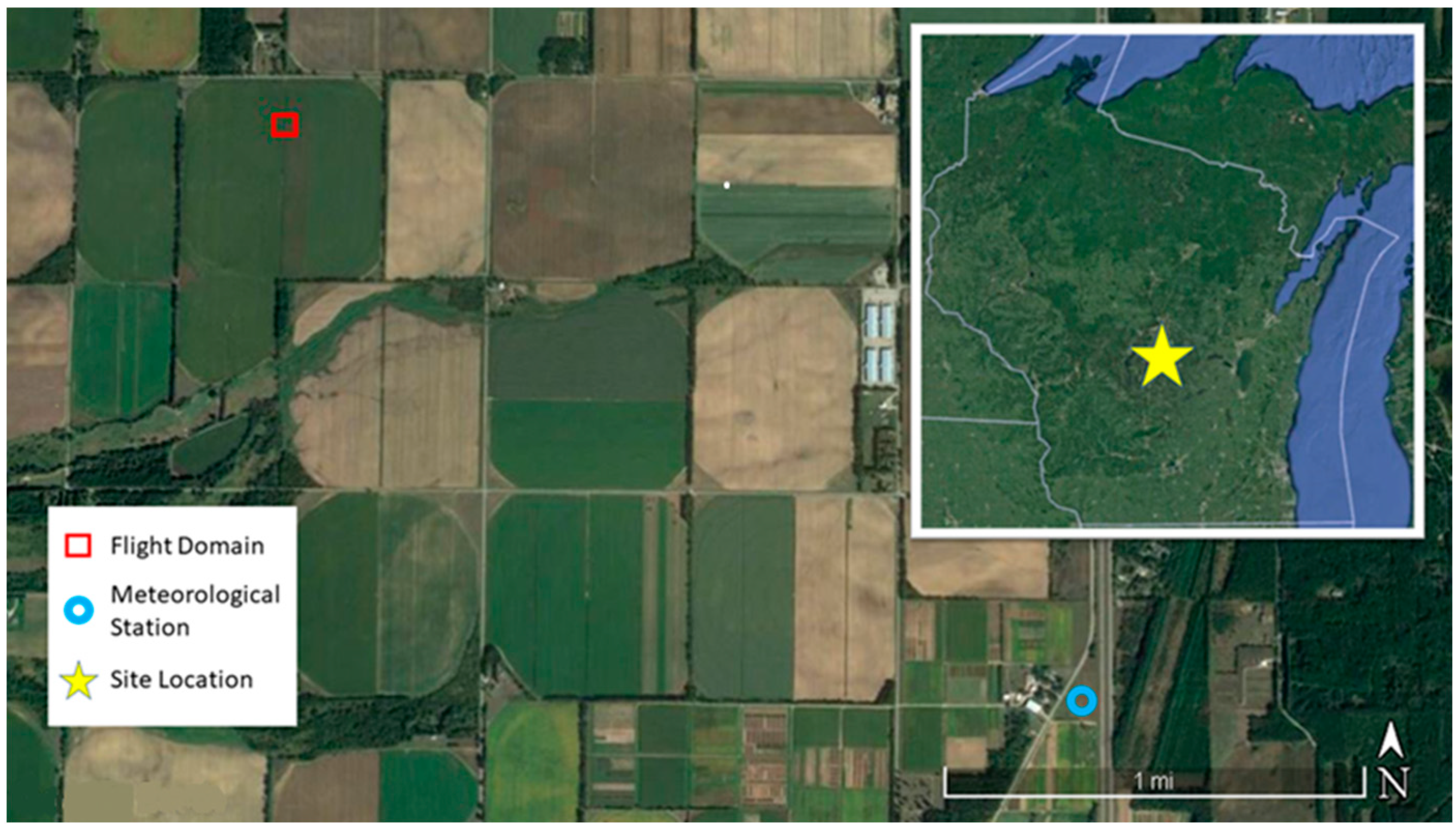
2.1. Site Description

Wisconsin is the third largest producer of potatoes in the United States, with 28,000 ha harvested and over 300 million USD in sales in 2019 [36,37]. Potatoes are one of the main agricultural products of the Wisconsin Central Sands. The Wisconsin Central Sands region (8860 km2) is known for its high sand content soil, humid climate, and high agricultural presence [38]. Temperatures in this region have an annual mean value of 6.6 °C with a mean January minimum of −19.2 °C and a mean August maximum of 27.1 °C [38]. On average, the area receives 830 mm of rain and 1140 mm of snow annually [38]. The storage capacity of the highly conductive sand aquifer and annual precipitation makes the area prime agricultural land. However, widespread agriculture and strong surface-ground water connection have led to water quality and groundwater depletion issues [39]. Namely, there are challenges with increasing groundwater nitrate concentrations, shallow private wells not being able to access water, and groundwater dependent surface waterbodies going dry [39]. Recent studies have shown that a reduction in frequency and magnitude of groundwater pumping for irrigation could reduce the impacts on nearby surface water in the Central Sands by reducing the amount of nitrate leached and runoff from the soil [28,40]. Precision irrigation has the potential to maintain agricultural productivity while reducing the magnitude and frequency of groundwater pumping in this region.
Drone imagery and ground reference data were collected to map ET from a 0.65-ha subsection of a 7.28-ha potato field in the Wisconsin Central Sands during the 2019 growing season (Figure 1). The subsection was centered around an Eddy Covariance system to capture the flux tower’s footprint (Section 2.7). Meteorological data were collected 3.9 km away from the field site (Section 2.5). Drone imagery and ground references were taken in partnership with an 11,000-ha commercial potato and vegetable farm. The field was planted 25 April, uniformly irrigated using a center pivot system, vine killed 18 August, and harvested 7 September. It rained almost weekly during the growing season and had a daily average reference ET of 3.62 mm, with a max of 5.30 mm on 10 July and a minimum of 0.96 mm on 26 August (Figure 2 and Figure 3). Little spatial variability was expected in the domain due to its flatness and relatively homogenous loamy sand soil.

2.2. Drone Missions and Data Processing

Eight mission sets were flown over the 2019 growing season with three different altitude (90, 60, and 30 m) flights per mission set (Table 1). Flight mission sets were scheduled to occur once a week during the least cloudy and windy day. We collected imagery over a 0.65-ha subsection of the field surrounding the Eddy Covariance tower (Figure 1). Thermal and multispectral data were collected with an 80% front and side overlap using an Altum combined multispectral-thermal camera (Micasense Inc., Seattle, WA, USA), mounted on a Matrice 210 RTK quadcopter (Shenzhen DJI Sciences and Technologies Ltd., Shenzen, Guangdong, China). The Altum camera captures five multispectral bands centered at 475, 560, 668, 717, and 842 nm. The multispectral data were captured at a resolution of 3.88, 2.59, and 1.29 cm for 90, 60, and 30 m, respectively. The Altum camera’s thermal sensor is centered at 11,000 nm. The thermal imagery was captured at a resolution of 60.9, 40.6, and 20.3 cm for 90, 60, 30 m, respectively. Atmospheric corrections were not conducted on the thermal imagery due to the low elevation of the flights. Rather, the differences between the thermal imagery and ground truth data points were used in the Monte Carlo uncertainty estimation procedure to help understand whether corrections are needed for low elevation remote sensing.
We processed images via the Micasense Altum processing workflow recommended for use with Agisoft Metashape Professional (Agisoft LLC, St. Petersburg, Russia). The multispectral data were calibrated in Metashape using images of a reflectance calibration panel (Micasense Inc., Seattle, WA, USA) before and after every flight. Images were then aligned geographically with high accuracy settings. A dense cloud was created using medium quality and aggressive depth filtering. A DEM was created from the dense cloud, and then used the surface for the ortho-mosaics. The ortho-mosaics were exported as geotiff files. The changes in viewing angle with elevation were considered negligible due to the low elevation of the flights and the short height of the potato canopy [41].

2.3. Thermal Ground Reference

Thermal ground reference data were collected for six of the eight mission sets. Samples were taken in four locations (three vegetation, one bare soil) immediately following the last flight in the mission set. Surface temperature values were collected using a Thermo Fisher handheld infrared thermometer (Thermo Fisher Scientific, Waltham, MA, USA). Five samples were taken at the top of the canopy (orthogonal) and averaged at each location for the six mission sets. We extracted remotely sensed temperature values using the average temperature of the 1.5 m diameter circle surrounding the ground reference sampling location. The ground reference temperatures and corresponding remotely sensed temperature values were used to calculate root mean square error (RMSE) for each flight elevation. RMSE values were 3.78, 4.42, and 3.44 °C for 90, 60, and 30 m respectively (Appendix A, Figure A1). July 8th had the highest RMSE values, while August 6th and 8th had the lowest RMSE values (Appendix A, Table A1). Atmospheric calibration was bypassed to assess uncertainty using ground reference comparisons for Monte Carlo Analyses.

2.4. Crop Phenology

We estimated leaf area index (LAI) and height values per pixel using established empirical models with the Enhanced Vegetative Index (EVI) developed for potato in the Wisconsin Central Sands region [2]. The multispectral images were aggregated to 5-m resolution to represent both plants and soils in each pixel [33]. EVI was computed from the aggregated imagery. The residual error from the empirical model was used to create ensemble data for Monte Carlo analyses. The LAI and height layers were disaggregated to the size of the thermal values and used to generate ET maps to restore resolution to the model while still accounting for the lowest resolution input (thermal).

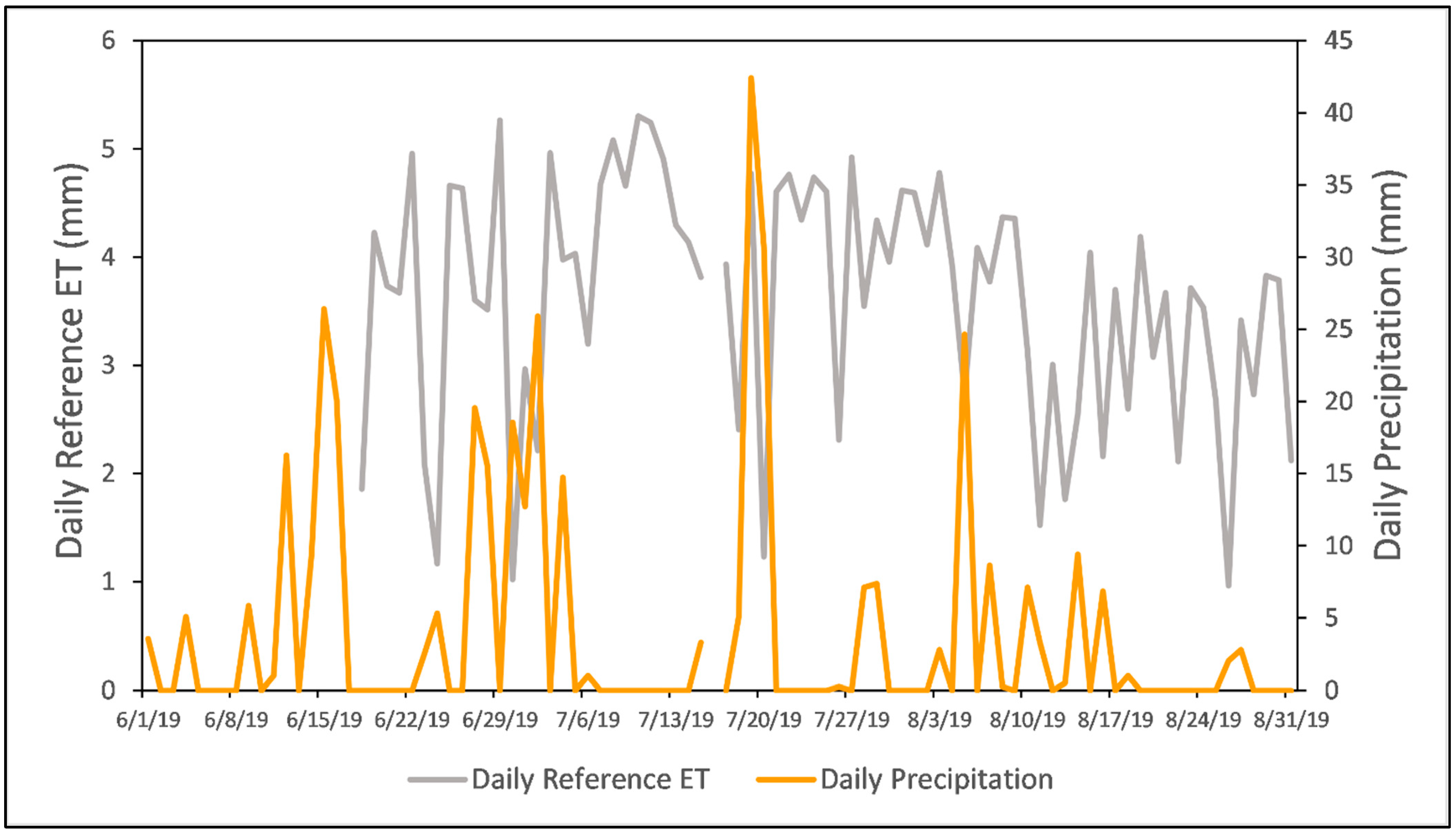
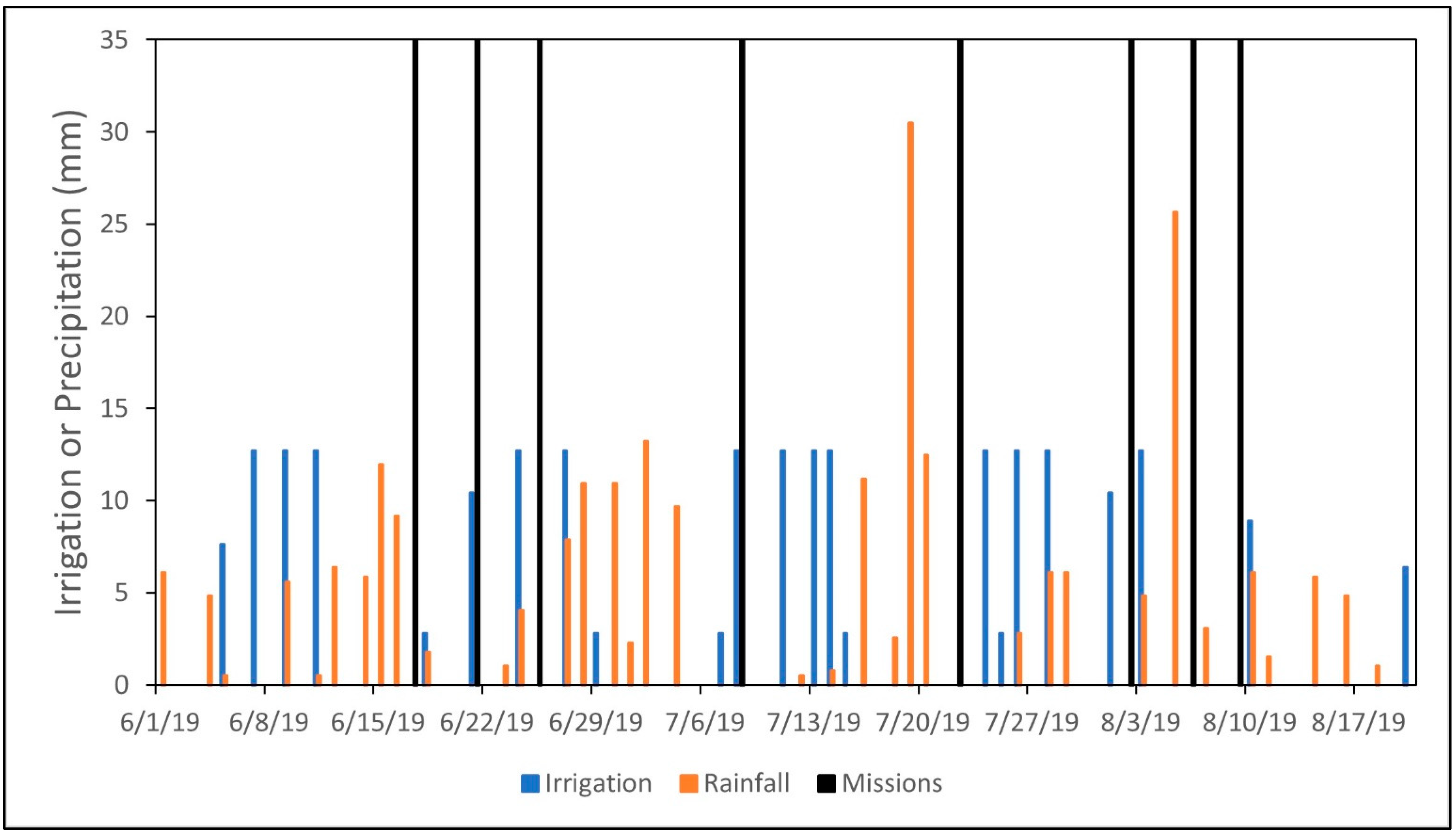
2.5. Meteorological Data Collection

Meteorological data were collected at a nearby weather station operated by the University of Wisconsin–Madison and University of Michigan. The meteorological data were used from this station rather than the EC tower due to crucial differences in temporal resolution and a more continuous dataset. Instruments measuring air temperature (HMP155A; Campbell Scientific, Logan, UT, USA), relative humidity (HMP155A; Campbell Scientific, Logan, UT, USA), and solar radiation (LI200R Pyranometer; LI-COR Biosciences, Lincoln, NE, USA) were mounted 1.5 m above a short grass surface. The instrument measuring wind speed (03002-L Wind Sentry Set; Campbell Scientific, Logan, UT, USA) was mounted 3 m above a short grass surface. Measurements for air temperature, relative humidity, and wind speed were taken every 5 min. Measurements for solar radiation were recorded hourly. Vapor pressure was calculated using relative humidity and air temperature values. Daily reference ET was reported from the station [42].
Mean values of air temperature, vapor pressure, and wind speed used in HRMET model simulations were extracted 30 min before and after the midpoint of the respective mission set. The values for solar radiation used in HRMET model simulations were linearly regressed and calculated using the measurements recorded (1) closest to the middle of the set, (2) proceeding recording, and (3) following recording. Uncertainty in air temperature, vapor pressure, and wind speed was estimated using the standard deviation of the measurements before and after takeoff. Uncertainty in solar radiation was estimated as the root mean square error (RMSE) of the linear regression.

2.6. Remotely Sensed Maps of ET and Uncertainty Estimation

Many remotely sensed ET models rely on the designation of ‘hot’ and ‘cold’ pixels that scale the minimum and maximum limits of ET within the domain [21,23]. While this scaling requires less input data [33] and reduces uncertainty from meteorological inputs [29], it can create challenges in homogenous agricultural fields [43]. Complicating things further, irrigated fields often aim to minimize water stress, making it harder to find ‘hot’ pixels for scaling, especially in humid regions. This lack of a ‘hot’ pixel can be particularly troublesome for precision irrigation with small imagery domains. We use the High-Resolution Mapping of Evapotranspiration (HRMET) model to mitigate some of these issues. HRMET is a singular, process-based energy model that uses canopy characteristics, surface temperature, and local meteorological data to estimate latent heat flux as the residual of the energy balance, and then converted to ET. Available energy for vegetation and soil is calculated using a two-source energy algorithm while sensible heat flux is iteratively solved as a single source for each pixel. This iteration removes the need to find ‘hot’ and ‘cold’ pixels, making it useful for developing ET maps for small fields. HRMET was developed for airplane imagery and has already been used in potatoes [9], peas (Pisum sativum), sweet corn (Zea mays), and field corn (Zea mays) [43].
ET maps were generated for each flight using a version of the HRMET model calibrated for potatoes in R Studio (RStudio, Boston, MA, USA). For information on the HRMET model, refer to Zipper and Lohiede, 2014 [43]. HRMET is an open-source model and the code for R and MATLAB are available at https://github.com/samzipper/HRMET (Last accessed on 20 January 2020). HRMET is run on a pixel-by-pixel basis. The three flight elevations had the same flight domain but had different pixel counts depending on resolution. Pixel count averaged 2,120,000, 4,890,000, and 20,740,000 for the 90, 60, and 30 m flights, respectively. HRMET ET values were assessed by mean, median, minimum, and maximum across the spatial footprint of the EC tower.
We estimated the influence of uncertainty from the model inputs using a Monte Carlo approach [44]. The mean and standard deviation of all spatial, meteorological, and empirical inputs were used to create an ensemble of input data based on the standard normal distribution. HRMET was run using randomly generated values from the normal distribution ensemble until 95% of the pixels had reach stability for at least 10 runs. A running average and standard deviation were calculated after every iteration. Stability was defined when the average value for a pixel was within 0.1% its value in the regular HRMET run. It took on average 300 iterations to reach scene stability. We used the Monte Carlo analyses to generate maps of the standard deviation of ET per pixel. We ran the analyses using an Intel i9 processor (Intel, Santa Clara, CA, USA), an Nvidia Quadro P620 graphics card (Nvidia, Santa Clara, CA, USA), and 64GB Corsair Vengeance LPX RAM (Corsair, Fremont, CA, USA). Because of the long runtime for these calculations (taking approximately 1.5 weeks for 90 m missions, one month for test 60 m missions, and 3 months for test 30 m missions) and no further insights from test 60 and 30 m missions, we limited Monte Carlo analyses to only the 90 m missions. Each HRMET input and its data sources are described in Table 2.
We calculated a Relative ET index [43] to compare intra-plot variability between different flights. Relative ET was calculated by linearly normalizing the mean to the 5th and the 95th percentile for each mission. Values closer to 1 indicate the highest ET rates within the domain and the values closer to 0 indicate the lowest ET rates within the domain.

2.7. Eddy Covariance

Fluxes of sensible and latent heat were collected using an Eddy Covariance (EC) tower at a half-hourly rate [45]. Water vapor, heat, and turbulent winds were measured with a Campbell Scientific, Inc. IRGASON, along with standard meteorological, surface radiation, and soil measurements. The instruments were located at 2.7 m height and were approximated to have a footprint radius ten times the instrument height (r = 27.4 m) [46]. The time series was aggregated to an hourly scale to match the time scale of the HRMET ET algorithm. The EC ET data were then linearly regressed using the recording closest to each flight’s midpoint and the recording before and after, to find the ET value nearest the flight. Ground heat flux was not collected during this period and the fluxes were assumed to have a closure of 10% from the random turbulent uncertainty [47].

3. Results

3.1. Spatial Features

Notable features are present in the imagery domain (see any raster figure, i.e., Figure 4). The thick, vertical line that bisects the domain is the field road providing access to the center pivot irrigation system. The thin, horizontal line that bisects the imagery domain is a track line left behind by the center pivot system. The squared shape bare soil location in the bottom left corner of the domain is an area that the potato planter missed; this area was later planted and the canopy closed (as can be seen in the later mission sets). These features may or may not be related to changes in ET. We observed and attributed some miscellaneous dark spots that appear on some days but not at all the flight elevations as overhead cloud interference.

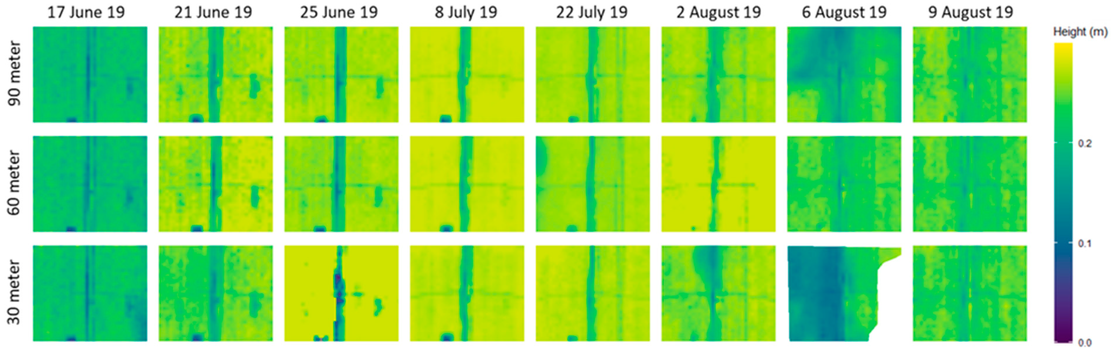
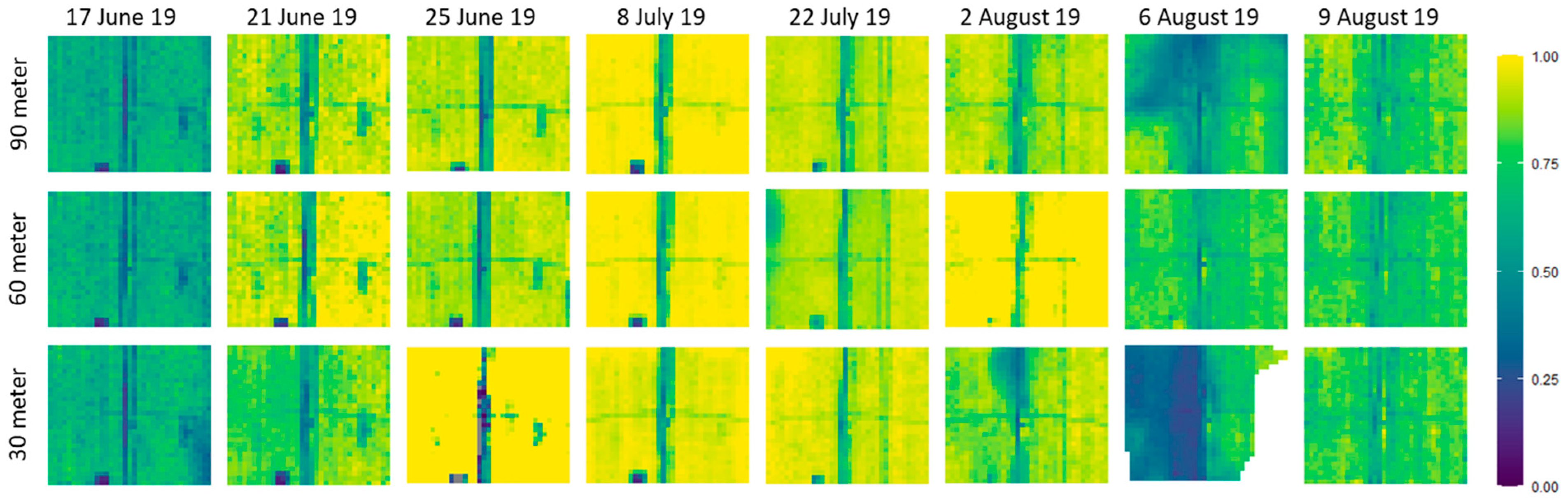
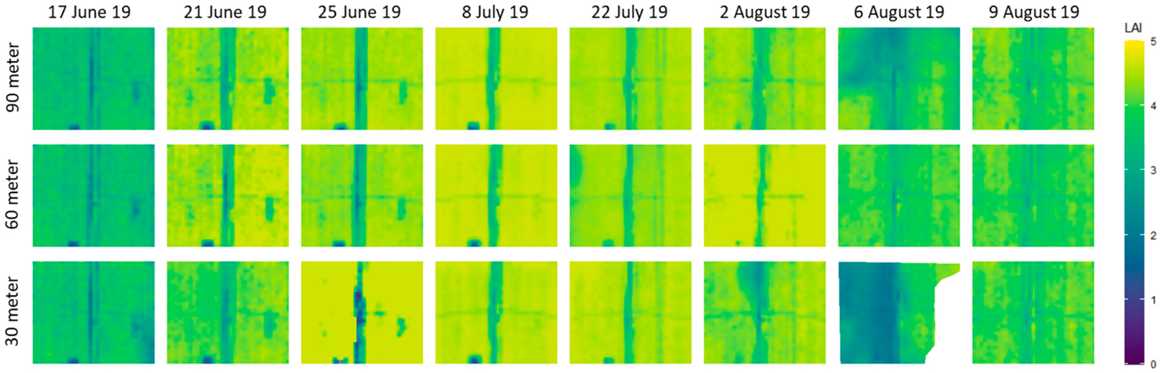
3.2. EVI, Height and LAI

Values for EVI peaked on 8 July, decreasing steadily with the senescence of the potato canopy (Appendix B, Figure A2. There was little variability in EVI between flight elevations on days that were not already associated with scattered clouds. As flight elevations decreased, there was an increase in the ability to visually discern individual rows, but no new unique features appeared in the EVI imagery with increased resolution.
Values for height peaked on 8 July at 0.28 m, decreasing steadily with the senescence of the potato canopy (Appendix B, Figure A3). There was little variability between flight elevations on days that were not already associated with scattered clouds. As flight elevation decreased there was an increase in visually discernable individual rows based on their height, but no new unique features appear. Across cropped areas, the values visually appear to be more homogenous than EVI.
Values for LAI peaked on the 8 July at 4.75 m2 m−2, only slightly decreasing with the senescence of the potato canopy (Figure 4). There was little variability between flight elevations on days that were not already associated with scattered clouds. As flight elevation decreased there was an increase visually discernable individual rows based on the higher resolution of the bands prior to aggregation, but no new unique features appear. Across cropped areas, the values visually appear to be more homogenous than EVI, especially around their peak days.

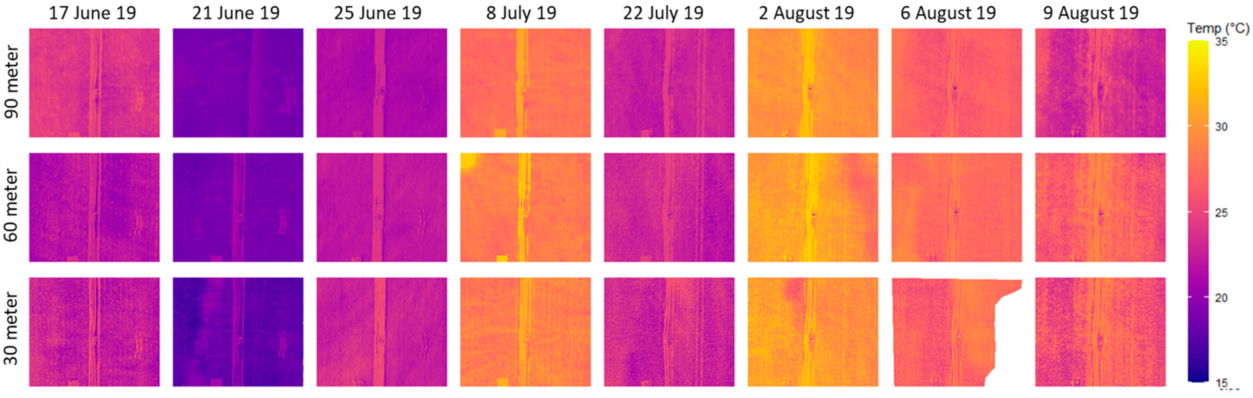
3.3. Surface Temperature
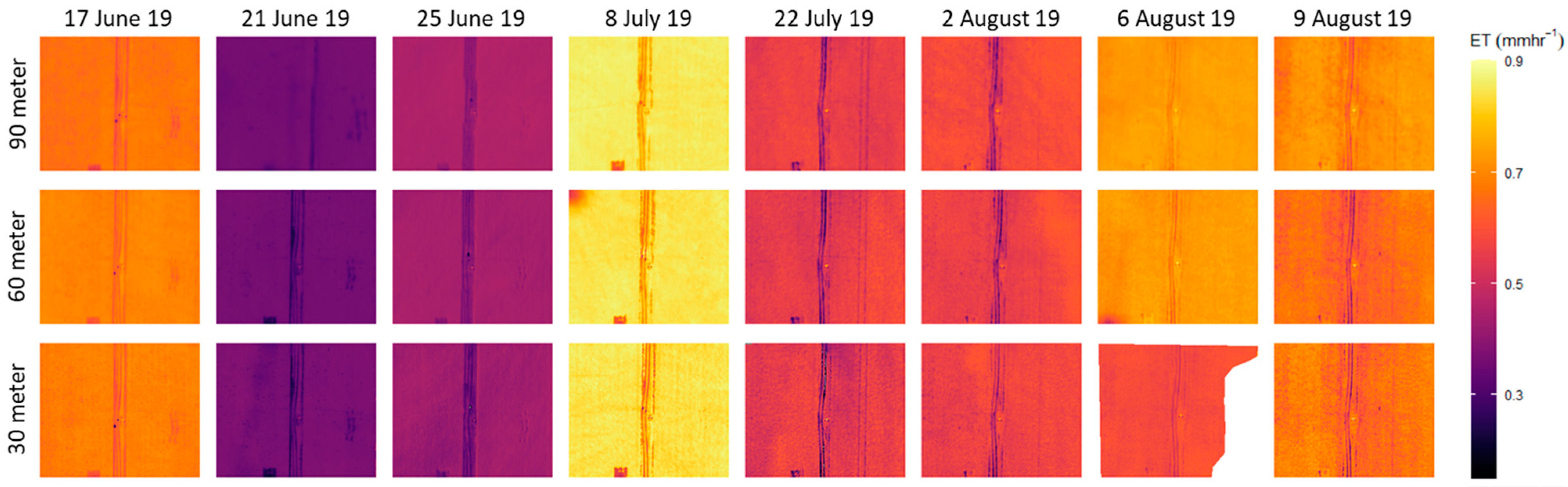
Surface temperatures were highest on 2 August at 34 °C and lowest on 21 June at 16 °C (Figure 5). The 21 June mission set took place after a 35-mm irrigation event that occurred the morning of the flight. Surface temperature values stayed constant with the change in flight elevation. Cloud cover had little visual impact on the plots between the different elevations. As flight elevation decreased there was an increase in visually discernable individual rows (Figure 5), but no new unique features appear. Missions that had either irrigation the day of flights (21 June and 8 July) or heavy rainfall within 24 h prior to the flights (6 August), had the least variability of surface temperature throughout the scene.

3.4. HRMET ET

HRMET ET was highest on 8 July at 0.9 mm h−1 and lowest on 21 June at 0.3 mm h−1 (Figure 6). ET value ranges had no observable differences across the flight elevations, with the exception of the mission sets that had cloud interference (Table 3). As flight elevation decreased, there was an increase in visually discernable individual rows and their differences in ET. Missions that had either irrigation earlier on the day of flights (21 June and 8 July) or heavy rainfall 24 h prior to the flights (6 August), had the least variability of ET throughout the scene.
The relative ET plots accentuate the variability in the cropped areas of the plot (Figure 7). Individual rows become more visible, but at the cost of the cloud interference also becoming more visible (6 August, 60 m). There are variations in relative ET across the scene between elevations for the same mission sets, but these variations are not seen in the HRMET ET plots (17 June, 21 June, 25 June, and 2 August). Lower elevation flights provide greater delineation between higher and lower values. This replaces averaged pixels with more ‘extreme’ values. While across the scene, the values remain the same, new patterns emerge with higher resolution.

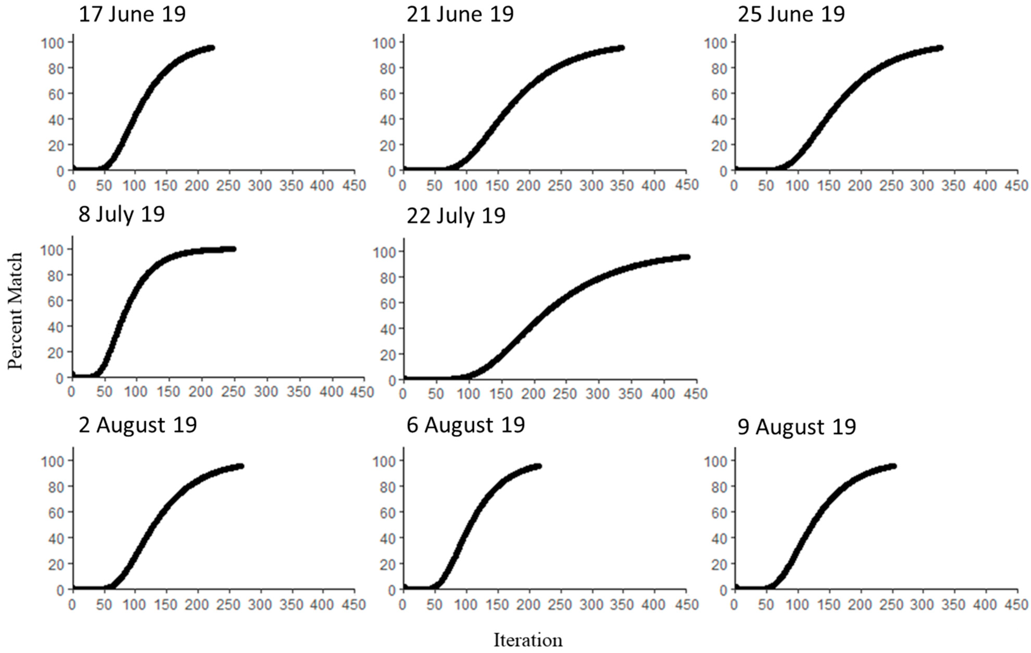
3.5. Monte Carlo Uncertainty Assessment

The number of Monte Carlo simulations required to reach 95% match stability varied, though all 90-m missions converged on a solution (Figure 8). The days with greater variability in meteorological inputs tended to require more iterations to reach stability (Figure 8). Days with variable solar radiation, such as 22 July, took almost 450 iterations. Days with low solar radiation and low wind speeds, such as 17 June and 6 August, took only 225 iterations. Using the Monte Carlo analyses, we found a per pixel standard deviation of 0.02–0.11 mm h−1 across all 90-m ET maps (Figure 9). Most missions were visually comparable with the notable exception of 22 July which had observably higher standard deviation. The spatial patterns in uncertainty across the 90-m missions signify that the dominant sources of uncertainty in the imagery are the spatial data. This would be the uncertainty of the spatial inputs (LAI, height, surface temperature) rather than the cameras. Uncertainty originating from the camera would have resulted in a more uniform distribution. The bare soil portions of the domain tended to show higher uncertainty. The higher uncertainty and meteorological variability on 22 July indicate that the differences in ET may be more related to temporal difference than plant stomatal control. The days with lower uncertainty and meteorological variability (21 June and 8 July) indicate that the differences in ET may be based in plant stomatal control.

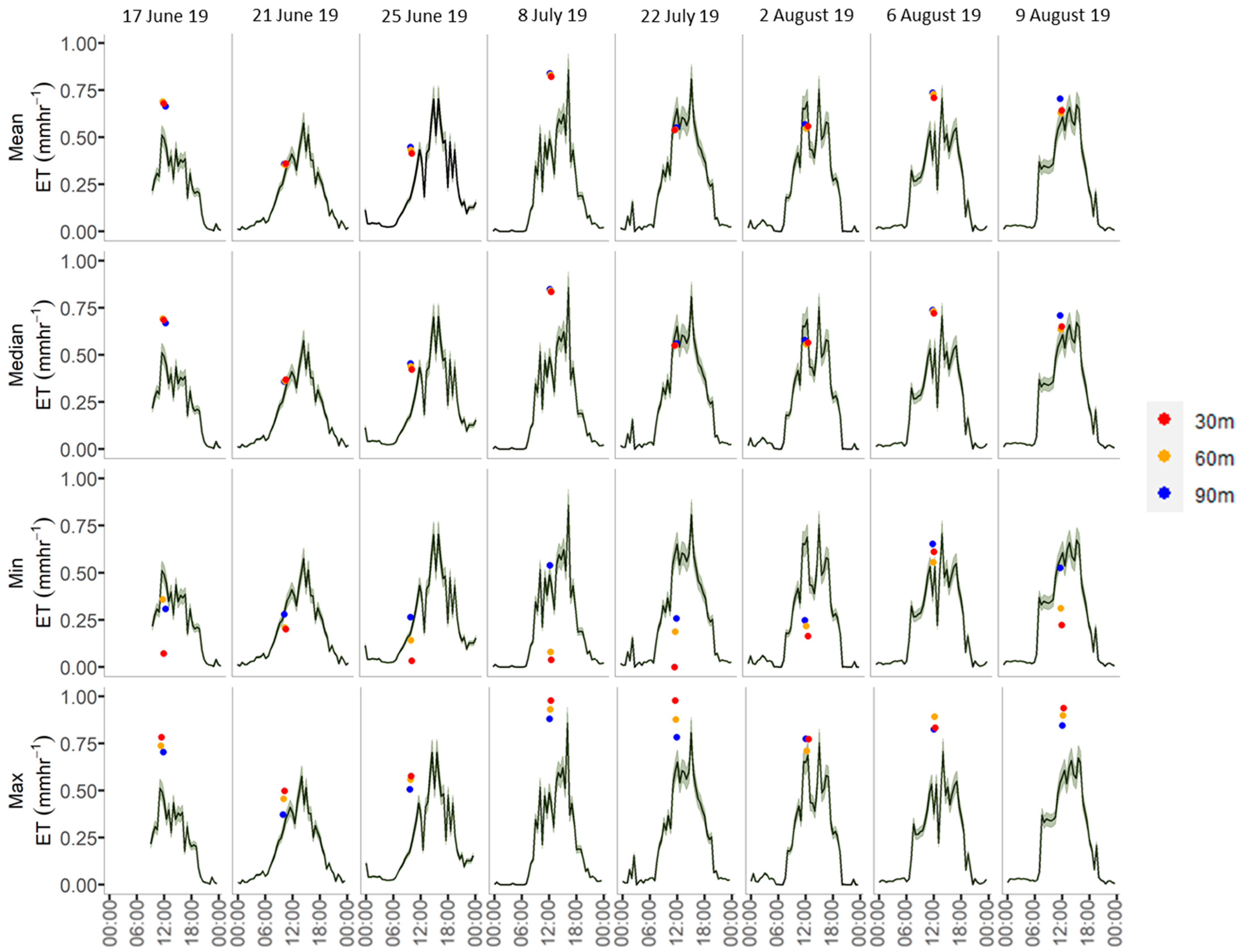
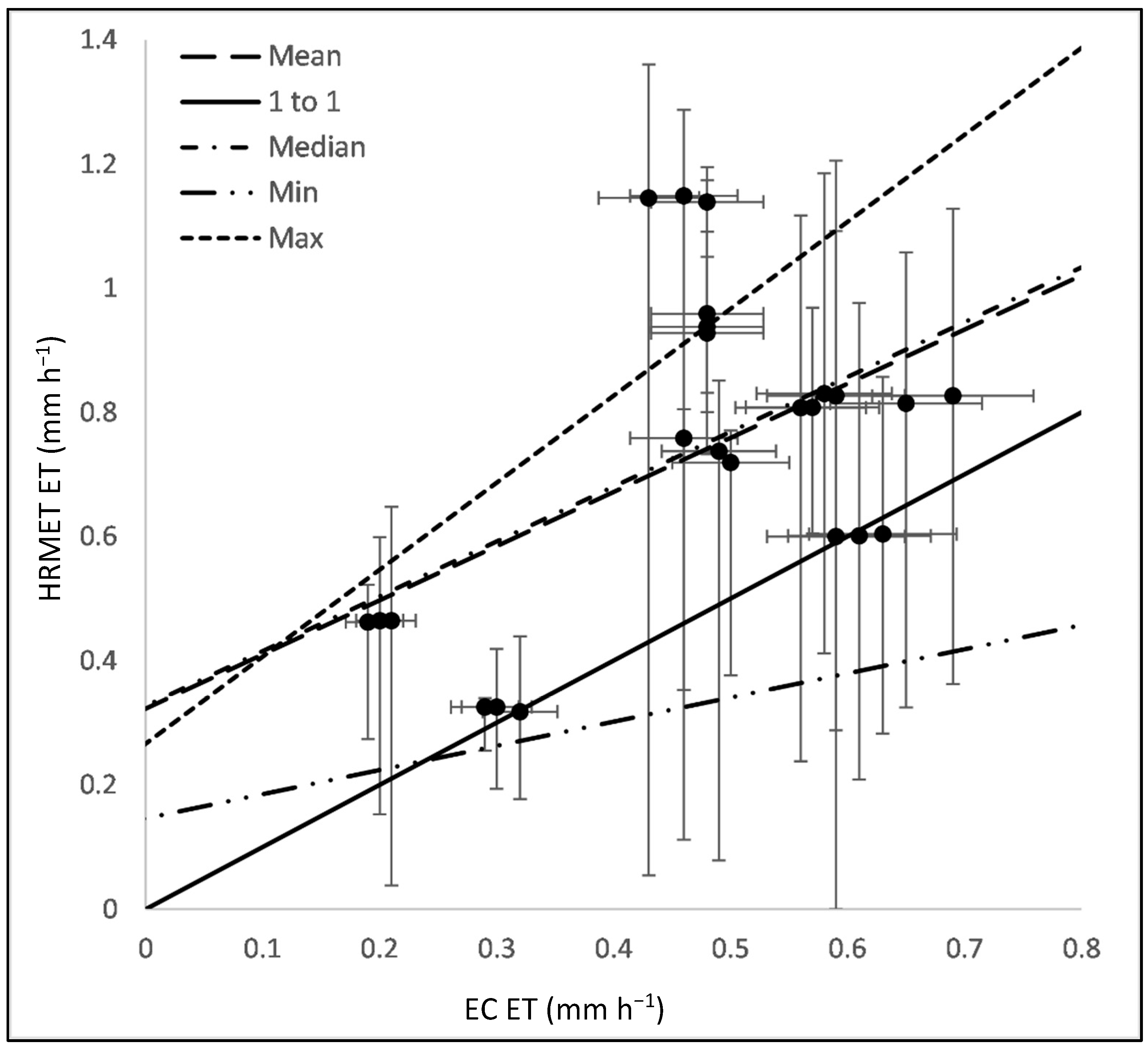
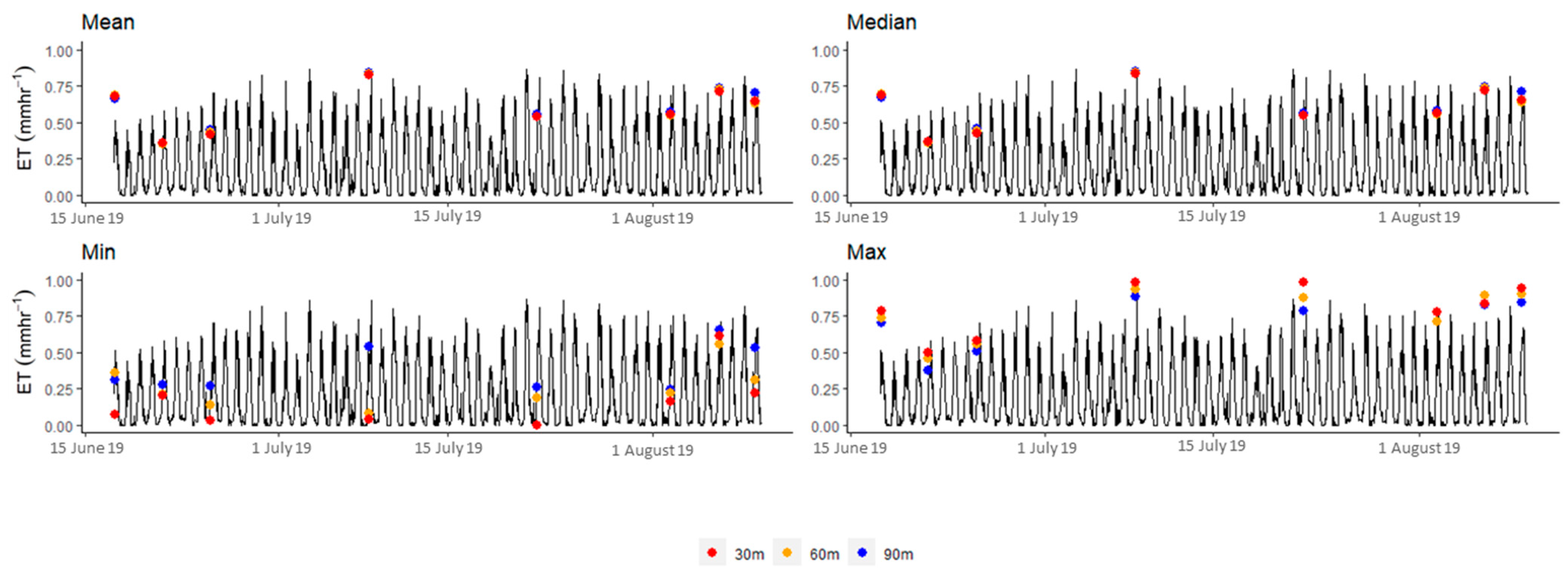
3.6. Comparison of HRMET with Eddy Covariance

Across the season, the HRMET ET values fall within the range of the EC ET values (Figure 10). The mean and median of the HRMET values performed closest to the EC ET when compared to those minimum and maximum HRMET values from the scene. Mean HRMET values tended to have higher ET values than the EC tower by a mean of 0.27, a median of 0.25, a maximum of 0.72, and a minimum of <0.00 mm h−1 across the season (Figure 11 and Figure 12). The 30 m flight on 21 June had the closest HRMET and EC values with a difference of <0.01 mm h−1. The 30 m flight on 8 July had the highest difference in HRMET and EC values with a difference of 0.71 mm h−1. There were no observable differences in how ET maps from the different mission elevations compared to the EC data. The mean and median HRMET values performed similarly with an RMSE of 0.21 mm h−1 (Figure 12, Table 4). The minimum HRMET values had the weakest relationship (R2 of 0.05) and an RMSE of 0.29 mm h−1 (Figure 12, Table 3). The maximum HRMET values had the strongest relationship (R2 of 0.48) and an RMSE 0.32 mm h−1 (Figure 12, Table 4).
The 21 June and 8 July missions followed irrigation events (~10 and ~13 mm, respectively, Figure 3). The 6 August mission had heavy rain the day before the flights (~25 mm). The 21 June mission matched the EC values well while the 8 July and 6 August missions did not match the EC values well. The 21 June and 2 August HRMET mean and median ET values were the closest to the EC ET values with a difference of 0.04 and 0.17 mm h−1, respectively. In contrast, the 17 June, 8 July, and 6 August HRMET mean and median ET values had the largest differences from corresponding EC ET values of 0.25, 0.70, and 0.47 mm h−1, respectively. The 21 June and 6 August minimum HRMET runs performed the nearest to the EC values with differences of 0.09 and 0.30 mm h−1, respectively. The 8 July and 22 July minimum HRMET runs performed the furthest from the EC ET values with differences of 0.31, and 0.42 mm h−1, respectively. The 17 June and 2 August maximum HRMET runs performed the nearest to the EC values with differences of 0.31 and 0.46 mm h−1, respectively. The 8 July and 6 August maximum HRMET runs performed the furthest from the EC ET values with differences of 0.82 and 0.62 mm h−1, respectively.

4. Discussion

4.1. Comparison of HRMET and Eddy Covariance ET Estimates

The mean and median HRMET ET values in this study were generally higher than the EC ET values, which is consistent with past work that has found EC ET values to be lower than remotely sensed ET values from the pySEBAL, SEBs, and TSEB models [12,19]. However, our findings differ from other findings where the EC values were higher than the METRIC, MODIS, and Gleam ET values [19,30,34]. The pySEBAL, and SEBS models tend to underestimate actual ET as a result of not having true ‘cold’ pixels in the model domain [19]. The lack of ‘cold’ pixels would result in an underestimation of ET because the ‘cold’ pixel sets the upper limit. In contrast, HRMET does not use a ‘hot’ and ‘cold’ pixel approach, so the reason for overestimation is not related to the absence of true well-watered pixels in the scene. Alternatively, this study’s assumption that the EC system’s area of influence (footprint) is a static circle has also been identified as a source of inconsistency in studies comparing remotely sensed ET maps to EC measurements [48]. The EC system’s area of influence changes with wind direction and atmospheric stability, which would change the appropriate HRMET domain to compare with EC measurements for a given day [48]. Future work could compute individual EC footprints for each mission set to improve scaling for comparisons. Sometimes EC measurements display a lack of closure of the energy budget which could indicate an underestimation bias of 10% that contributed to difference between HRMET and EC values [49].
The input data for HRMET and the EC tower have a difference in ideal climatic conditions. Namely, EC systems perform better with greater wind speeds while the surface temperature imagery collected for HRMET increases in variability with increasing wind and gust speeds. For example, 8 July had a lower wind speed (0.8 m s−1) and the EC ET was 0.71 mm h−1 lower than the HRMET values. For the EC time series on 8 July, there is an observable reduction in ET that coincides with a reduction in wind speed.
Though we assumed that there is at least ~10% uncertainty in EC estimates because of turbulent sampling or energy budget closure issues [47], we did not quantify the uncertainty associated with EC estimates used for HRMET comparison, nor the uncertainties inherent in the HRMET model assumptions and equations. Additionally, the scales at which the two are collected could have an impact on how outliers impact the overall value. The EC tower gives a single value while HRMET multiple values for the same area. We compared mean, median, max, and min HRMET values to the EC ET values, but there may be other spatially weighted approaches, such as a footprint cutoff approach [50], that could be more appropriate for these comparisons. Finally, despite our attempts to match HRMET and EC estimates in time, the difference in capture period (30-min for EC and variable for drone-based image capture) makes it difficult to associate the ET values to the right moment in time. This can be particularly challenging for comparison because of dynamic atmospheric conditions. Nevertheless, our overall results show consistent temporal patterns across the two approaches, confirming the suitability of drone for ET mapping in the Midwest United States.

4.2. Adapting the HRMET Model for Very High-Resolution Imagery

HRMET was initially developed for use with aerial imagery (1–30 m2 scale), and because of this, there are issues of scale when applying it to drone imagery (0.2–0.6 m2). The resolution for the input multispectral imagery is too fine to calculate a vegetation index (VI) needed to use the regression to estimate LAI and crop height, because VIs are canopy scale measurements while the drone imagery is on the leaf scale. The imagery can be aggregated to calculate the VI and then disaggregated to maintain resolution, but the disconnect in principle must be noted. A possible solution to this would be directly measure LAI and crop height by using relationships with RGB reflectance values or using point cloud estimations, respectively [51,52].
Another issue with the input VI raster was the false presence of LAI and crop height in bare soil spots (as can be seen in the field road of Figure 3 and Figure 4). This stems from empirical model extrapolation at very low values. This results in an overestimation of ET in bare soil areas by estimating transpiration for pixels where there is no vegetation present. A possible solution to this issue would be to use two source energy balance model that would separately estimate soil evaporation, though this may increase computational needs [53].

4.3. How High to Fly?

Overall, there were no observable differences or trends between the EVI, height, temperature, and ET estimates from the different mission elevations. There is a marginal increase in resolution and detectable features with the lower elevation flights. The influence of these additional detectable features is present at all elevations. At higher elevations, the additional features become incorporated in larger mixed pixels. Further study is needed to determine the potential for using the additional detectable features as a tool for creating management zones [54]. However, low elevation flights can create challenges with photo alignment when using multi-lens cameras [55]. Lower elevations also take longer to fly, reducing the coverage area as well as introducing the opportunity for solar radiative changes. Low elevation images also have smaller ground area to capture unique tie-points which can cause issues with aligning the imagery. In this case, there was not a need to have imagery resolution beyond what can be managed computationally. Additionally, precision irrigation can only be done as efficiently as the irrigation infrastructure in place. Based on these challenges associated with lower-elevation flights, we suggest that the flight elevation be no lower than the elevation necessary to capture the finest characteristics of the field upon which management is actionable.
Higher resolution ET maps could be more useful for perennial crops where there is high individual crop value (e.g., orchards, vineyards). The higher resolution would allow for better monitoring of water stress, health, and pests in individual trees, bushes, or vines [55,56,57]. There may be more considerations for tall orchard crops where the aspect may have a greater impact on photogrammetry and would emphasize the need to study specific mission planning to optimize image capture.

4.4. When to Fly?

When collecting drone imagery, it is best to follow current best practices and collect imagery around solar noon, fly the same time for every flight, use at least 70% front and side overlap, fly under 12 m s−1 winds, avoid clouds, and avoid collecting imagery while the field is being actively irrigated [58,59]. In practice, it is hard to meet these conditions while attempting to collect imagery on a frequent schedule. To accommodate for these demands, we collected imagery with the best conditions that were present at the time. As such, there were some conditions that were not ideal. Three missions of note were 21 June, 8 July, and 6 August where the mission domain had either just been irrigated or experienced a heavy rain event. This would cause an increase in the evaporation portion of ET and higher ET values [60,61]. However, these three days did not have the same response; 8 July and 6 August had relatively high ET values (range mm h−1) while 21 June had relatively low ET values (range mm h−1). This could be because the 21 June mission set was conducted early in the day (9:30 am) where the evaporative demand was not yet at a maximum value. Alternatively, the 8 July and 6 August mission sets were collected near solar noon at peak evaporation demand.

4.5. Limitations

Some of the conditions in which the imagery was collected resulted in the introduction of uncertainty. Discrepancies between the thermal imagery and the ground reference data (Appendix A) could indicate atmospheric interference [62]. In particular, the wind speed and variation could have temporarily cooled the surface at a given location during the capture period. The RMSE values for this imagery were higher but comparable to Simpson et al., 2021 (~3 °C); however, their data were collected over a large, controlled grass area that avoided the ‘spot size effect’ which led to more stable and precise readings.
Thermal ground reference data were collected after the final flight in the mission set. This led to a 30-min latency between the start of the first flight and the first ground reference point taken. Depending on how stable the surface temperature was during the sampling time, this could have introduced uncertainty. Thermal ground references of maximum and minimum temperatures were not collected, which could have set the scale for the surface temperature range [28]. The thermal ground references were also collected as spot measurements but were compared to the mean of a 1.5 m diameter circle from the thermal imagery. For future work, we recommend a larger thermal ground reference area (>3 m2) that would appear in several pixels of thermal imagery collected at 90-m. The June 21st and 25th flights were flown earlier than recommended, potentially introducing more variability in solar radiation [29]. Clouds were not always avoidable (22 July) causing variability in solar radiation across the elevations and in individual plots. This variability can cause ‘dark’ low reflectance spots on the imagery under cloudy conditions [30].
There are more causes of spatial variability of ET to address. The variability we observed cannot be fully attributed to stomatal control. For future work, we recommend using spatially-explicit measurements of stomatal conductance and photosynthesis to complement tower-based comparisons [63].

5. Conclusions

Drone-based remote sensing offers the ability to rapidly generate ET maps within a season that can be used to make in-season decisions. The use of ETmaps with precision irrigation has the potential to reduce water use and nitrogen loss from agricultural fields. The High Resolution Mapping of Evapotranspiration (HRMET) model has been previously used for mapping ET from Midwestern potatoes using aerial imagery. We found that HRMET may also be useful for ET mapping with drone imagery if the flights are collected under optimal conditions. We evaluated whether there was an increase in insightful information from ET maps created using imagery collected at 90, 60, or 30 m. Though there were some additional detectable features observed from low elevation flights, the tradeoff in resources and computation does not currently justify low elevation flights for annual vegetable crops in the Midwest USA. Spatial data were the predominant source of uncertainty in the HRMET model. High solar radiation variability or low wind speeds were the biggest driver in the difference between HRMET and Eddy Covariance (EC) ET estimates. Uncertainty maps are an underutilized tool that have the potential to evaluate the strengths and weaknesses of high-resolution ET maps. Going forward, further application to the HRMET model, or models like it, could prove beneficial, especially for precision irrigation crops that may not have the ideal ‘hot’ and ‘cold’ pixels. Further study is needed to understand how HRMET performs in other climates outside the Midwest United States.

Author Contributions

Conceptualization, M.A.N., S.C.Z., J.P., L.A.E. and A.J.C.; methodology, L.A.E., A.J.C., M.A.N. and A.T.; eddy covariance, A.T. and A.R.D.; software, L.A.E., M.A.N. and S.C.Z.; comparison, L.A.E., K.T.P.U., M.A.N., A.R.D. and A.T.; formal analysis, L.A.E., M.A.N. and K.T.P.U.; investigation, L.A.E. and M.A.N.; resources, M.A.N., A.R.D., S.C.Z. and J.P.; writing—original draft preparation, L.A.E.; writing—review and editing, M.A.N.; visualization, L.A.E.; supervision, M.A.N., A.R.D. and J.P.; project administration, M.A.N. and J.P.; funding acquisition, M.A.N., J.P., S.C.Z., A.R.D. and A.T. All authors have read and agreed to the published version of the manuscript.

Funding

M.A.N., S.C.Z., J.P. acknowledge funding from the Wisconsin Potato and Vegetation Growers Association Water Task Force. M.A.N. acknowledges the David H. Smith Conservation Research Fellowship. A.R.D. and A.T. acknowledge funding from the Wisconsin Potato and Vegetation Growers Association Water Task Force and the Wisconsin Department of Natural Resources to University of Wisconsin-Madison and the DOE Ameriflux Network Management Project.

Institutional Review Board Statement

Not applicable.

Informed Consent Statement

Not applicable.

Data Availability Statement

Eddy covariance flux tower data are available https://doi.org/10.17190/AMF/1617713 (Last accessed on 19 January 2022). Processed drone imagery available on request to L.A.E.

Acknowledgments

We acknowledge the support of J. Thom, UW-Madison, T. Houlihan, WPVGA, A. Ruzic, and J. Pavelski, Heartland Farms for partnership, operation, and maintenance of the flux tower. We would also like to acknowledge K. Lawton, J. Oestreich, and A. Doherty for computational support at UW-Stevens Point. We would like to thank A. Mandel and D. Young for photogrammetry support at UC-Davis.

Conflicts of Interest

The authors declare no conflict of interest. The funders had no role in the design of the study; in the collection, analyses, or interpretation of data; in the writing of the manuscript, or in the decision to publish the results.

Appendix A

Figure A1. Thermal ground reference data vs. surface temperature values remotely collected with Micasense Altum. Ground reference data were collected within half an hour of mission launch.
Remotesensing 14 01660 g0a1
Table A1. Root Mean Square Error (RMSE) of thermal ground reference data vs. surface temperature (°C) values collected with Micasense Altum. Ground reference data were collected within half an hour of mission launch.
Elevation (m)25 June 20198 July 201922 July 20192 August 20196 August 20199 August 2019
902.004.714.281.522.725.63
602.448.422.774.512.042.93
303.596.411.641.202.452.60

Appendix B

Figure A2. Enhanced Vegetation Index (EVI, unitless) raster maps for each mission. Maps are linearly scaled to the same color bar.
Remotesensing 14 01660 g0a2
Figure A3. Canopy height (m) raster maps derived from Enhanced Vegetation Index for each mission.
Remotesensing 14 01660 g0a3

References

  1. US Geological Survey. Estimated Use of Water in the United States in 2015; USGS: Reston, WA, USA, 2015.
  2. Park, M. Fertilizers and the environment. Nutr. Cycl. Agroecosyst. 1999, 55, 117–121. [Google Scholar] [CrossRef]
  3. Bai, Y.-C.; Chang, Y.-Y.; Hussain, M.; Lu, B.; Zhang, J.-P.; Song, X.-B.; Lei, X.-S.; Pei, D. Soil Chemical and Microbiological Properties Are Changed by Long-Term Chemical Fertilizers That limit Ecosystems Functioning. Microorganisms 2020, 8, 694. [Google Scholar] [CrossRef] [PubMed]
  4. Liu, D.J.; Feng, J.X. Precision irrigation and its prospect analysis. Water Sav. Irrig. 2006, 43, 43–44. [Google Scholar]
  5. Sadler, E.J.; Evans, R.G.; Stone, K.C.; Camp, C.R. Opportunities for conservation with precision irrigation. J. Soil Water Conserv. 2005, 60, 371–379. [Google Scholar]
  6. Barzegari, M.; Sepaskhah, A.R.; Ahmadi, S.H. Irrigation and nitrogen managements affect nitrogen leaching and root yield of sugar beet. Nutr. Cycl. Agroecosyst. 2017, 108, 211–230. [Google Scholar] [CrossRef]
  7. Hedley, C.; Yule, I.; Bradbury, S. Analysis of potential benefits of precision irrigation for variable soils at five pastoral and arable production sites in New Zealand. In Proceedings of the 19th World Soil Congress, Brisbane, Australia, 6–9 August 2010. [Google Scholar]
  8. Liang, Z.; Liu, X.; Xiong, J.; Xiao, J. Water Allocation and Integrative Management of Precision Irrigation: A Systematic Review. Water 2020, 12, 3135. [Google Scholar] [CrossRef]
  9. Nocco, M.A.; Zipper, S.C.; Booth, E.G.; Cummings, C.R.; Ii, S.P.L.; Kucharik, C.J. Combining Evapotranspiration and Soil Apparent Electrical Conductivity Mapping to Identify Potential Precision Irrigation Benefits. Remote Sens. 2019, 11, 2460. [Google Scholar] [CrossRef] [Green Version]
  10. King, B.A.; Stark, J.C.; Wall, R.W. Comparison of site-specific and conventional uniform irrigation management for potatoes. Appl. Eng. Agric. 2006, 22, 677–688. [Google Scholar] [CrossRef]
  11. Asfaw, E.; Suryabhagavan, K.V.; Argaw, M. Soil salinity modeling and mapping using remote sensing and GIS: The case of Wonji sugar cane irrigation farm, Ethiopia. J. Saudi Soc. Agric. Sci. 2016, 17, 250–258. [Google Scholar] [CrossRef] [Green Version]
  12. Hoffmann, H.; Nieto, H.; Jensen, R.; Guzinski, R.; Zarco-Tejada, P.; Friborg, T. Estimating evaporation with thermal UAV data and two-source energy balance models. Hydrol. Earth Syst. Sci. 2016, 20, 697–713. [Google Scholar] [CrossRef] [Green Version]
  13. Rud, R.; Cohen, Y.; Alchanatis, V.; Levi, A.; Brikman, R.; Shenderey, C.; Heuer, B.; Markovitch, T.; Dar, Z.; Rosen, C.; et al. Crop water stress index derived from multi-year ground and aerial thermal images as an indicator of potato water status. Precis. Agric. 2014, 15, 273–289. [Google Scholar] [CrossRef]
  14. Khanal, S.; Fulton, J.; Shearer, S. An overview of current and potential applications of thermal remote sensing in precision agriculture. Comput. Electron. Agric. 2017, 139, 22–32. [Google Scholar] [CrossRef]
  15. Barbedo, J.G.A. A Review on the Use of Unmanned Aerial Vehicles and Imaging Sensors for Monitoring and Assessing Plant Stresses. Drones 2019, 3, 40. [Google Scholar] [CrossRef] [Green Version]
  16. Cazaurang, F.; Cohen, K.; Kumar, M. Multi-Rotor Platform-Based UAV Systems; Elsevier: Amsterdam, The Netherlands, 2020. [Google Scholar]
  17. Calera, A.; Campos, I.; Osann, A.; D’Urso, G.; Menenti, M. Remote sensing for crop water management: From ET modelling to services for the end users. Sensors 2017, 17, 1104. [Google Scholar] [CrossRef] [PubMed] [Green Version]
  18. Kustas, W.P.; Norman, J.M. Use of remote sensing for evapotranspiration monitoring over land surfaces. Hydrol. Sci. J. 1996, 41, 495–516. [Google Scholar] [CrossRef]
  19. Xue, J.; Bali, K.M.; Light, S.; Hessels, T.; Kisekka, I. Evaluation of remote sensing-based evapotranspiration models against surface renewal in almonds, tomatoes and maize. Agric. Water Manag. 2020, 238, 106228. [Google Scholar] [CrossRef]
  20. Wandera, L.; Mallick, K.; Kiely, G.; Roupsard, O.; Peichl, M.; Magliulo, V. Upscaling instantaneous to daily evapotranspiration using modelled daily shortwave radiation for remote sensing applications: An artificial neural network approach. Hydrol. Earth Syst. Sci. 2017, 21, 197–215. [Google Scholar] [CrossRef] [Green Version]
  21. Norman, J.M.; Kustas, W.P.; Humes, K.S. Source approach for estimating soil and vegetation energy fluxes in observations of directional radiometric surface temperature. Agric. For. Meteorol. 1995, 77, 263–293. [Google Scholar] [CrossRef]
  22. Yang, Y.; Shang, S. A hybrid dual-source scheme and trapezoid framework-based evapotranspiration model (HTEM) using satellite images: Algorithm and model test. J. Geophys. Res. Atmos. 2013, 118, 2284–2300. [Google Scholar] [CrossRef]
  23. Bastiaanssen, W.G.M.; Meneti, M.; Feddes, R.A.; Holtslag, A.A.M. A remote sensing surface energy balance algorithm for land (SEBAL). Hydrology 1998, 212–213, 198–212. [Google Scholar] [CrossRef]
  24. Feng, J.; Wang, Z. A satellite-based energy balance algorithm with reference dry and wet limits. Int. J. Remote Sens. 2013, 34, 2925–2946. [Google Scholar] [CrossRef]
  25. Haboudane, D.; Miller, J.R.; Pattey, E.; Zarco-Tejada, P.J.; Strachan, I.B. Hyperspectral vegetation indices and novel algorithms for predicting green LAI of crop canopies: Modeling and validation in the context of precision agriculture. Remote Sens. Environ. 2004, 90, 337–352. [Google Scholar] [CrossRef]
  26. Espinoza, C.Z.; Khot, L.R.; Sankaran, S.; Jacoby, P.W. High resolution multispectral and thermal remote sensing-based water stress assessment in subsurface irrigated grapevines. Remote Sens. 2017, 9, 961. [Google Scholar] [CrossRef] [Green Version]
  27. Gerhards, M.; Rock, G.; Schlerf, M.; Udelhoven, T. Water stress detection in potato plants using leaf temperature, emissivity, and reflectance. Int. J. Appl. Earth Obs. Geoinf. 2016, 53, 27–39. [Google Scholar] [CrossRef]
  28. Nocco, M.A.; Kraft, G.J.; Loheide, S.P.; Kucharik, C.J. Drivers of Potential Recharge from Irrigated Agroecosystems in the Wisconsin Central Sands. Vadose Zone J. 2018, 17, 170008. [Google Scholar] [CrossRef] [Green Version]
  29. Allen, R.G.; Tasumi, M.; Trezza, R. Satellite-Based Energy Balance for Mapping Evapotranspiration with Internalized Calibration (METRIC)—Model. J. Irrig. Drain. Eng. 2007, 133, 395–406. [Google Scholar] [CrossRef]
  30. Talsma, C.J.; Good, S.P.; Jimenez, C.; Martens, B.; Fisher, J.B.; Miralles, D.; McCabe, M.; Purdy, A.J. Partitioning of evapotranspiration in remote sensing-based models. Agric. For. Meteorol. 2018, 260–261, 131–143. [Google Scholar] [CrossRef]
  31. Smail, R.; Nocco, M.; Colquhoun, J.; Wang, Y. Remotely-sensed water budgets for agriculture in the upper midwestern United States. Agric. Water Manag. 2021, 258, 107187. [Google Scholar] [CrossRef]
  32. Nassar, A.; Torres-Rua, A.; Kustas, W.; Nieto, H.; McKee, M.; Hipps, L.; Stevens, D.; Alfieri, J.; Prueger, J.; Alsina, M.M.; et al. Influence of model grid size on the estimation of surface fluxes using the two source energy balance model and sUAS imagery in vineyards. Remote Sens. 2020, 12, 342. [Google Scholar] [CrossRef] [Green Version]
  33. Xia, T.; Kustas, W.P.; Anderson, M.C.; Alfieri, J.G.; Gao, F.; McKee, L.; Prueger, J.H.; Geli, H.M.E.; Neale, C.M.U.; Sanchez, L.; et al. Mapping evapotranspiration with high-resolution aircraft imagery over vineyards using one-and two-source modeling schemes. Hydrol. Earth Syst. Sci. 2016, 20, 1523–1545. [Google Scholar] [CrossRef] [Green Version]
  34. Mokhtari, A.; Ahmadi, A.; Daccache, A.; Dreschsler, K. Actual Evapotranspiration from UAV Images: A Multi-Sensor Data Fusion Approach. Remote Sens. 2021, 13, 2315. [Google Scholar] [CrossRef]
  35. Nassar, A.; Torres-Rua, A.; Hipps, L.; Kustas, W.; McKee, M.; Stevens, D.; Nieto, H.; Keller, D.; Gowing, I.; Coopmans, C. Using Remote Sensing to Estimate Scales of Spatial Heterogeneity to Analyze Evapotranspiration Modeling in a Natural Ecosystem. Remote Sens. 2022, 14, 372. [Google Scholar] [CrossRef]
  36. USDA. United States Summary and State Data. In 2017 Census of Agriculture; USDA: Washington, DC, USA, 2019. [Google Scholar]
  37. USDA. Wisconsin Ag News—Potatoes; USDA: Washington, DC, USA, 2020.
  38. WI-DNR. Central Sand Plains Ecological Landscape. In The Ecological Landscapes of Wisconsin: An Assessment of Ecological Resources and a Guide to Planning Sustainable Management; WI-DNR: Madison, WI, USA, 2014; 108p. [Google Scholar]
  39. Kraft, G.J.; Mechenich, D.J. Groundwater Pumping Effects on Groundwater Levels, Lake Levels, and Streamflows in the Wisconsin Central Sands; Center for Watershed Science and Education College of Natural Resources: Madison, WI, USA, 2010. [Google Scholar]
  40. Fienen, M.N.; Bradbury, K.R.; Kniffin, M.; Barlow, P.M. Depletion Mapping and Constrained Optimization to Support Managing Groundwater Extraction. Groundwater 2018, 56, 18–31. [Google Scholar] [CrossRef] [PubMed]
  41. Tempfli, K.; Huurneman, G.; Bakker, W.; Janssen, L.L.; Feringa, W.F.; Gieske, A.S.M.; Grabmaier, K.A.; Hecker, C.A.; Horn, J.A.; Kerle, N.; et al. Principles of Remote Sensing; International Institute for Geo-Information Science and Earth Observation: Enschede, The Netherlands, 2009. [Google Scholar]
  42. Allen, R.; Pereira, L.; Raes, D.; Smith, M. Crop Evapotranspiration: Guidelines for Computing Crop Water Requirments; Food and Agriculture Organization of the United Nations: Rome, Italy, 1998. [Google Scholar]
  43. Zipper, S.C.; Loheide, S.P. Using evapotranspiration to assess drought sensitivity on a subfield scale with HRMET, a high resolution surface energy balance model. Agric. For. Meteorol. 2014, 197, 91–102. [Google Scholar] [CrossRef]
  44. Hammersley, J.; Handscomb, D. Monte Carlo Methods; Chapman and Hall: London, UK, 1979. [Google Scholar]
  45. Desai, A.R. AmeriFlux US-CS3 Central Sands Irrigated Agricultural Field; Wisconsin Department of Natural Resources: Madison, WI, USA, 2020.
  46. Arriga, N.; Rannik, Ü.; Aubinet, M.; Carrara, A.; Vesala, T.; Papale, D. Experimental validation of footprint models for eddy covariance CO2 flux measurements above grassland by means of natural and artificial tracers. Agric. For. Meteorol. 2017, 242, 75–84. [Google Scholar] [CrossRef]
  47. Rannik, Ü.; Peltola, O.; Mammarella, I. Random uncertainties of flux measurements by the eddy covariance technique. Atmos. Meas. Tech. 2016, 9, 5163–5181. [Google Scholar] [CrossRef] [Green Version]
  48. Horst, T.W.; Weil, J.C. Footprint estimation for scalar flux measurements in the atmospheric surface layer. Boundary-Layer Meteorol. 1992, 59, 279–296. [Google Scholar] [CrossRef]
  49. Mauder, M.; Foken, T.; Cuxart, J. Surface-Energy-Balance Closure over Land: A Review. Bound.-Layer Meteorol. 2020, 177, 395–426. [Google Scholar] [CrossRef]
  50. Nassar, A.; Torres-Rua, A.F.; Kustas, W.P.; Nieto, H.; McKee, M.; Hipps, L.E.; Alfieri, J.G.; Prueger, J.H.; Alsina, M.M.; McKee, L.G.; et al. To what extend does the Eddy Covariance footprint cutoff influence the estimation of surface energy fluxes using two source energy balance model and high-resolution imagery in commercial vineyards? In Autonomous Air and Ground Sensing Systems for Agricultural Optimization and Phenotyping V; International Society for Optics and Photonics: Bellingham, WA, USA, 2020. [Google Scholar]
  51. Raj, R.; Walker, J.P.; Pingale, R.; Nandan, R.; Naik, B.; Jagarlapudi, A. Leaf area index estimation using top-of-canopy airborne RGB images. Int. J. Appl. Earth Obs. Geoinf. 2020, 96, 102282. [Google Scholar] [CrossRef]
  52. Haala, N. Multiray Photogrammetry and Dense Image Matching. In Photogrammetric Week; VDE: Berlin, Germany, 2011. [Google Scholar]
  53. Zhang, N.; Wang, M.; Wang, N. Precision agriculture—A worldwide overview. Comput. Electron. Agric. 2002, 36, 113–132. [Google Scholar] [CrossRef]
  54. Sánchez, J.M.; López-Urrea, R.; Rubio, E.; González-Piqueras, J.; Caselles, V. Assessing crop coefficients of sunflower and canola using two-source energy balance and thermal radiometry. Agric. Water Manag. 2014, 137, 23–29. [Google Scholar] [CrossRef]
  55. Capturing from Low Altitudes and from a Fixed Point. Available online: https://support.micasense.com/hc/en-us/articles/360045449134-Capturing-from-low-altitudes-and-from-a-fixed-point (accessed on 15 September 2021).
  56. Gonzalez-Dugo, V.; Zarco-Tejada, P.; Nicolás, E.; Nortes, P.A.; Alarcón, J.J.; Intrigliolo, D.S.; Fereres, E.J.P.A. Using high resolution UAV thermal imagery to assessthe variability in the water status of five fruit tree specieswithin a commercial orchard. Nature 2018, 388, 539–547. [Google Scholar]
  57. Luedeling, E.; Hale, A.; Zhang, M.; Bentley, W.J.; Dharmasri, L.C. Remote sensing of spider mite damage in California peach orchards. Int. J. Appl. Earth Obs. Geoinf. 2009, 11, 244–255. [Google Scholar] [CrossRef]
  58. Fouche, P.S. The use of low-altitude infrared remote sensing for estimating stress conditions in tree crops. S. Afr. J. Sci. 1995, 91, 500–502. [Google Scholar]
  59. Gallego, J.; Carfagna, E.; Baruth, B. Accuracy, Objectivity and Efficiency of Remote Sensing for Agricultural Statistics. In Agricultural Survey Methods; Wiley: Hoboken, NJ, USA, 2008. [Google Scholar]
  60. Ozdogan, M.; Yang, Y.; Allez, G.; Cervantes, C. Remote Sensing of Irrigated Agriculture: Opportunities and Challenges. Remote Sens. 2010, 2, 2274–2304. [Google Scholar] [CrossRef] [Green Version]
  61. Li, Z.-L.; Tang, R.; Wan, Z.; Bi, Y.; Zhou, C.; Tang, B.; Yan, G.; Zhang, X. A Review of Current Methodologies for Regional Evapotranspiration Estimation from Remotely Sensed Data. Sensors 2009, 9, 3801–3853. [Google Scholar] [CrossRef] [Green Version]
  62. Simpson, J.; Holman, F.; Nieto, H.; Voelksch, I.; Mauder, M.; Klatt, J.; Fiener, P.; Kaplan, J. High spatial and temporal resolution energy flux mapping of different land covers using an off-the-shelf unmanned aerial system. Remote Sens. 2021, 13, 1286. [Google Scholar] [CrossRef]
  63. Ha, W.; Kolb, T.E.; Springer, A.E.; Dore, S.; O’Donnell, F.C.; Morales, R.M.; Lopez, S.M.; Koch, G.W. Evapotranspiration comparisons between eddy covariance measurements and meteorological and remote-sensing-based models in disturbed ponderosa pine forests. Ecohydrology 2014, 8, 1335–1350. [Google Scholar] [CrossRef]
Figure 1. Map of 2019 study site. Flight domain is centered around an EC tower. The meteorological station was located 3.9 km southeast of the site. Aerial imagery provided by Google Earth.
Remotesensing 14 01660 g001
Figure 2. Growing season daily timeseries of reference evapotranspiration (mm, left y-axis) and precipitation (mm, right y-axis) for 2019 from the University of Wisconsin–Madison research station in Hancock, WI. There was a gap in time series data on 17 July 2019.
Remotesensing 14 01660 g002
Figure 3. Growing season timeseries of irrigation (mm) and precipitation (mm) for 2019. Precipitation is in hourly increments and the timing of irrigation events are associated with the irrigation initiation (duration is not depicted). Mission sets are highlighted with black vertical lines. Imagery was not collected while the center pivot system was running.
Remotesensing 14 01660 g003
Figure 4. LAI (m2 m−2) raster maps derived from Enhanced Vegetation Index for each mission.
Remotesensing 14 01660 g004
Figure 5. Surface temperature (°C) raster maps for each mission.
Remotesensing 14 01660 g005
Figure 6. HRMET ET (mm h−1) raster maps for each mission.
Remotesensing 14 01660 g006
Figure 7. Relative ET raster maps for each mission based off HRMET-derived ET. Relative ET is the standardized ET using the plots 5th and 95th percentile as the boundaries.
Remotesensing 14 01660 g007
Figure 8. Percent scene match curves for Monte Carlo uncertainty analyses of HRMET-derived ET. Match determined as a pixel having an average value within 10% of the regular HRMET run.
Remotesensing 14 01660 g008
Figure 9. Standard deviation of HRMET-derived ET based on Monte Carlo analysis for each mission. Raster maps were only created for the 90 m elevation.
Remotesensing 14 01660 g009
Figure 10. Timeseries of EC ET (black line, mm h−1) compared to the instantaneous HRMET ET (points, mm h−1) for different flight elevations.
Remotesensing 14 01660 g010
Figure 11. Daily timeseries of EC ET (mm h−1) and instantaneous HRMET ET (mm h−1) across the 8 mission sets. A 10% buffer added to the EC time series.
Remotesensing 14 01660 g011
Figure 12. HRMET and EC ET regression between every flight mission from the 2019 growing season. One-to-one line added as reference to the plots. Slope, y-intercept, R2 and RMSE were calculated for the mean, median, minimum, and maximum HRMET ET values.
Remotesensing 14 01660 g012
Table 1. Remotely Piloted Mission Sets. Meteorological data were averaged values from 30-min before and after the midpoint of each flight mission. Standard deviations over this time period are listed within parentheses.
Mission SetDate (DOY)Flight Time (CST)Air
Temperature
(°C)
Wind Speed
(m s−1)
Solar
Radiation (W m−2)
Vapor Pressure (kPa)
117 June 2019 (170)11:11–11:5124.5 (0.2)1.7 (0.3)724.8 (0.7)0.8 (0.0)
221 June 2019 (172)9:52–10:1819.4 (0.2)1.4 (0.2)413.6 (2.7)1.0 (0.0)
325 June 2019 (176)9:31–9:5120.9 (0.8)1.7 (0.2)498.6 (0.1)1.5 (0.0)
48 July 2019 (189)12:03–12:2426.3 (0.4)0.9 (0.2)809.7 (3.3)1.7 (0.0)
522 July 2019 (203)11:25–12:5121.6 (0.6)3.5 (0.4)621.3 (16.1)1.3 (0.0)
62 August 2019 (214)11:58–12:4526.8 (0.3)1.1 (0.3)627.3 (4.3)1.9 (0.0)
76 August 2019 (218)11:57–12:3725.1 (0.4)1.4 (0.2)756.8 (5.2)2.1 (0.1)
89 August 2019 (221)11:57–12:1922.6 (0.4)2.1 (0.3)746.7 (4.4)1.4 (0.1)
Table 2. HRMET Inputs.
HRMET InputSpatial ResolutionFrequencySourceUncertainty Estimation Used in Monte Carlo Calculations
Canopy temperature20–60 cmInstantaneous Micasense Altum (Section 2.3)Ground reference data and drone collected data used to calculate Root mean square error (RMSE) of the regression (Section 2.4).
LAI1.3–3.9 cmInstantaneousMicasense Altum (Section 2.4)RMSE from the regression between LAI and EVI (Section 2.5)
Height1.3–3.9 cmInstantaneousMicasense Altum (Section 2.4)RMSE from the regression between height and EVI (Section 2.5)
Air temperatureFixed5-minMeteorological station (Section 2.5)Standard deviation of measurements 30-min before and after the takeoff time
Wind speed Fixed5-minMeteorological station (Section 2.5)Standard deviation of measurements 30-min before and after the takeoff time
Relative humidityFixed5-minMeteorological station (Section 2.5)Standard deviation of measurements 30-min before and after the takeoff time
Solar RadiationFixed1-hMeteorological station (Section 2.5)RMSE from the regression of the three measurements surrounding the takeoff time
AlbedoFixedFixedEmpirical (Section 2.6)0.05 standard deviation imposed
EmissivityFixedFixedEmpirical (Section 2.6)0.01 standard deviation imposed
Table 3. HRMET ET estimates (mm h−1) across the flight domain.
Elevation (m)17 June 201921 June 201925 June 20198 July
2019
22 July 20192 August 20196 August 20199 August 2019
900.76 (0.02)0.33 (0.01)0.46 (0.02)1.14 (0.03)0.60 (0.04)0.83 (0.04)0.94 (0.01)0.81 (0.03)
600.72 (0.02)0.33 (0.02)0.46 (0.02)1.15 (0.04)0.60 (0.04)0.81 (0.04)0.96 (0.02)0.83 (0.04)
300.74 (0.03)0.32 (0.03)0.46 (0.03)1.15 (0.05)0.60 (0.06)0.81 (0.04)0.93 (0.02)0.83 (0.05)
Table 4. Slope, y-intercept, R2, and RMSE values for the HRMEY and EC ET regression.
Slopey-InterceptR2RMSE
Mean0.870.320.260.21
Median0.880.330.260.21
Min0.390.150.050.29
Max1.400.270.480.32
Publisher’s Note: MDPI stays neutral with regard to jurisdictional claims in published maps and institutional affiliations.

