Article

An Estimation Method for PM2.5 Based on Aerosol Optical Depth Obtained from Remote Sensing Image Processing and Meteorological Factors

1
School of Physics and Electronic Technology, Liaoning Normal University, Dalian 116029, China
2
School of Geography, Liaoning Normal University, Dalian 116029, China
3
Key Laboratory of Digital Earth Science, Aerospace Information Research Institute, Chinese Academy of Sciences, Beijing 100094, China
*
Author to whom correspondence should be addressed.
Remote Sens. 2022, 14(7), 1617; https://doi.org/10.3390/rs14071617
Submission received: 25 February 2022 / Revised: 25 March 2022 / Accepted: 25 March 2022 / Published: 28 March 2022
(This article belongs to the Topic Climate Change and Environmental Sustainability)

Abstract

:
Understanding the spatiotemporal variations in the mass concentrations of particulate matter ≤2.5 µm (PM2.5) in size is important for controlling environmental pollution. Currently, ground measurement points of PM2.5 in China are relatively discrete, thereby limiting spatial coverage. Aerosol optical depth (AOD) data obtained from satellite remote sensing provide insights into spatiotemporal distributions for regional pollution sources. In this study, data from the Multi-Angle Implementation of Atmospheric Correction (MAIAC) AOD (1 km resolution) product from Moderate Resolution Imaging Spectroradiometer (MODIS) and hourly PM2.5 concentration ground measurements from 2015 to 2020 in Dalian, China were used. Although trends in PM2.5 and AOD were consistent over time, there were seasonal differences. Spatial distributions of AOD and PM2.5 were consistent (R2 = 0.922), with higher PM2.5 values in industrial areas. The method of cross-dividing the test set by year was adopted, with AOD and meteorological factors as the input variable and PM2.5 as the output variable. A backpropagation neural network (BPNN) model of joint cross-validation was established; the stability of the model was evaluated. The trend in the predicted values of BPNN was consistent with the monitored values; the estimation result of the BPNN with the introduction of meteorological factors is better; coefficient of determination (R2) and RMSE standard deviation (SD) between the predicted values and the monitored values in the test set were 0.663–0.752 and 0.01–0.05 μg/m3, respectively. The BPNN was simpler and the training time was shorter compared with those of a regression model and support vector regression (SVR). This study demonstrated that BPNN could be effectively applied to the MAIAC AOD data to estimate PM2.5 concentrations.

Graphical Abstract

1. Introduction

Particles with aerodynamic diameters of ≤2.5 μm are referred to as PM2.5, which encompasses a large variety of toxic and harmful substances. Environmental epidemiological studies have confirmed that long-term exposure to PM2.5 increases the incidence of cardiovascular and respiratory diseases [1,2]. Recent studies have determined that air pollutants are closely related to mortality associated with diabetes and increased obesity risk [3,4]. Therefore, monitoring PM2.5 mass concentrations and studying the causes of air pollution are important for safeguarding human health [5]. A time series of PM2.5 mass concentrations can be obtained using data derived from ground measurements. However, recent studies have reported that the spatial distribution of PM2.5 ground measurement points in China is limited [6,7]. With the growing development of satellite remote sensing technology, aerosol optical depth (AOD) obtained by remote sensing with a high spatial resolution and wide coverage has become an effective method to estimate PM2.5 mass concentration [8,9]. AOD is a powerful parameter for describing aerosol extinction and can be used as a proxy for atmospheric turbidity in air pollution research [10]. AOD data can be obtained from different sensors such as the Advanced Very High-Resolution Radiometer (AVHRR), Visible Infrared Imaging Radiometer Suite (VIIRS), Advanced Along-Track Scanning Radiometer (AATSR), and Moderate Resolution Imaging Spectroradiometer (MODIS). Wei et al. (2019) compared 11 global monthly AOD products with Aerosol Robotic Network (AERONET) sites, including four products from the European Space Agency’s Climate Change Initiative (AATSR-ADV, AATSR-EN, AATSR-ORAC, and AATSR-SU) and AVHRR, Multi-angle Imaging Spectro Radiometer (MISR), Terra and Aqua MODIS, POLarization and Directionality of the Earth’s Reflectance (POLDER), Sea-viewing Wide Field-of-view Sensor (SeaWiFS), and VIIRS products. The MODIS products show the best performance with the best evaluation metrics in describing the temporal aerosol variations [11]. Currently, most studies have employed AOD data based on the Dark Target (DT) algorithm [12], the Deep Blue (DB) algorithm [13], or a combination of Dark Target and Deep Blue (DTB) algorithm [14]. The 10 km AOD products have been widely used in PM2.5 estimation studies [15,16]; however, a 10 km resolution is not fine enough to resolve local variability [17,18,19]. Multi-angle implementation of atmospheric correction (MAIAC) is a new aerosol retrieval algorithm [20] that decouples aerosol and surface contributions using time series data. Jethva et al. (2019) verified and analyzed aerosols using the MAIAC algorithm on dark surfaces and showed that its accuracy was equal to or higher than that of the DT algorithm, and for bright surfaces, its accuracy was generally higher than that of the DB algorithm [21]. Li et al. (2020) found that compared with DT, DB, and DTB AOD products, the 1 km MAIAC AOD product obtained the best correspondence with AERONET measurements, with an overall coefficient of determination (R2) of 0.891 [22].
Numerous recent studies have inferred PM2.5 mass concentrations using AOD data obtained from satellite-based remote sensing [23,24,25,26]. The spatiotemporal distributions of PM2.5 are influenced by multiple factors such as meteorology [27], land use [28], and human activities [29]; changes in these factors can be estimated using satellite observations. Luo et al. (2021) analyzed the relationships between PM2.5 concentration and meteorological factors in Harbin. The results showed that relative humidity was positively correlated to PM2.5 concentration, while temperature, wind direction, and wind speed were negatively correlated to PM2.5 mass concentration [30]. Li et al. (2015) studied the spatiotemporal variations in AOD and PM2.5 mass concentrations in the USA and found that interannual changes in AOD and PM2.5 were highly consistent [31]. Initial studies used the atmospheric chemical transport model to simulate the scale factor between AOD and PM2.5, thereby enabling an estimation of PM2.5 mass concentrations from AOD [32]. Wang (2003) discussed the simple linear relationship between MODIS AOD on the Terra/Aqua satellites and hourly PM2.5 in Alabama, USA. The correlation coefficient (R) between AOD and PM2.5 was 0.70, while that for monthly comparisons was 0.91 and 0.95 for Terra and Aqua, respectively [33]. To improve model performance, meteorological parameters and land-use information were gradually incorporated into the model (R2 = 0.59–0.84), including a multiple regression model [34], linear mixed effect model [35], and geographically weighted regression model [36,37]. Although these models were of key importance in air pollution estimates, most statistical methods were difficult to find and displayed complex nonlinear laws. In recent years, significant progress has been made in the remote sensing inversion of PM2.5 based on machine learning, including support vector regression (SVR) [38], artificial neural network (ANN) model [39], and random forest model [40]. ANN is a nonlinear mapping model that can cope with systems that are difficult to describe using mathematical models and has the characteristics of parallel processing, self-adaptation, self-organization, associative memory, and approaching arbitrary nonlinearity. Gupta and Christopher (2009) used MODIS AOD data at 0.55 µm to estimate PM2.5 over the southeastern USA, based on an ANN that reduced the uncertainty of PM2.5 estimations from satellite data [41]. Their study demonstrated the potential for using ANNs for operational air quality monitoring. Guo et al. (2013) (R = 0.4–0.83) and Ni et al. (2018) (R2 = 0.54–0.68) established the backpropagation neural network (BPNN) to estimate PM2.5 using MODIS AOD, and the corresponding results showed that a PM2.5 estimation model based on MODIS AOD products could be effectively applied to PM2.5 monitoring under the framework of a BP network [42,43]. The structure of a BP neural network is divided into input layer, hidden layer, and output layer, and there are connection weights between neurons in adjacent layers. The hidden layer can be a single layer or a multi-layer, and the number of hidden layer nodes selected has an effect on the accuracy of BPNN. Although a BP neural network can realize any nonlinear fitting learning, BPNN also shows some drawbacks, such as the randomness of initial weights and thresholds. There is no systematic method for determining the number of hidden layer nodes at present [44]. Most studies, including those mentioned above, have ignored the randomness of the initial weight threshold. Without considering the extreme value of error, a single result is not sufficient to represent the final performance of the model. In addition, most studies determined the model parameters, including the number of neurons in the hidden layer, through a single and randomly divided verification set. Thus, there was no guarantee that the network parameters were optimal. Therefore, based on the analysis of the spatiotemporal correlation between AOD and PM2.5, this study aimed to solve the problems existing in BPNN by fine-tuning the dataset according to the annual cross-division; the model parameters were determined through joint cross-validation and evaluating the stability of the model. The BPNN was compared using a regression model and SVR to verify the performance advantages.

2. Materials and Methods
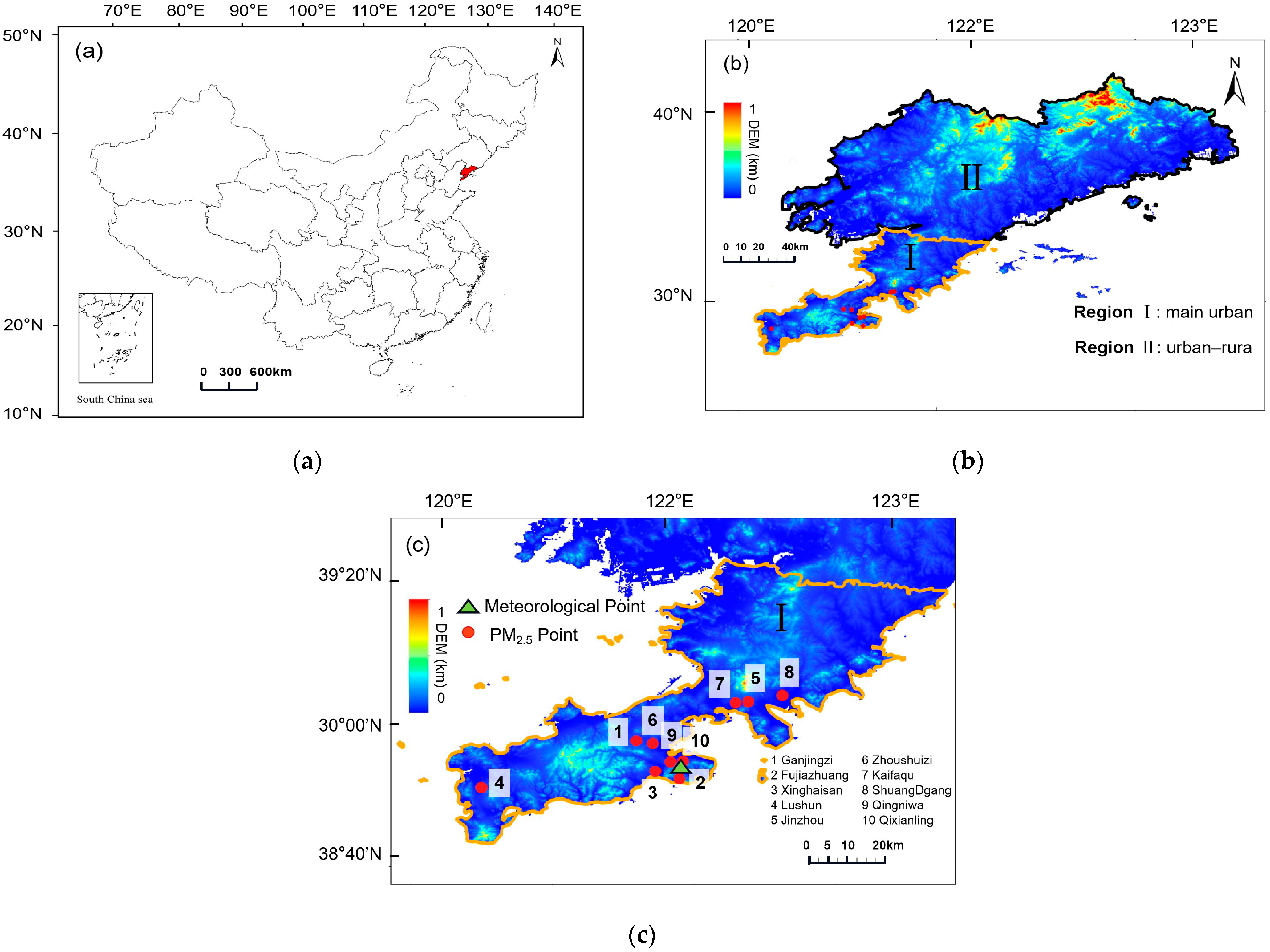
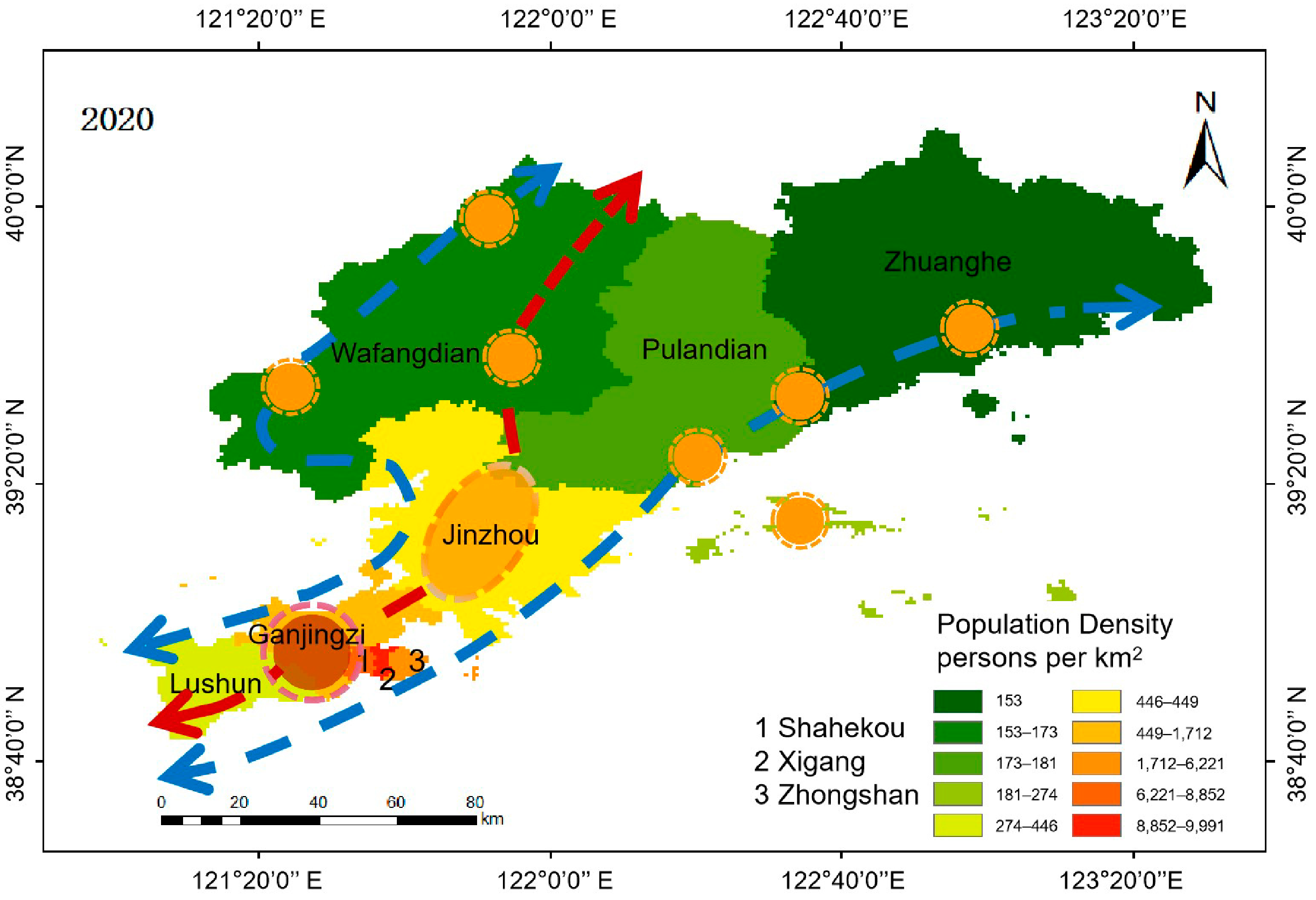
2.1. Study Area

Covering a wide area of 12,600 km2, Dalian spreads from a latitude of 38°43′N to 40°10′N and a longitude of 120°58′E to 123°31′E. As shown in Figure 1a, Dalian is a city with three sides surrounded by sea, located at the southernmost point of Northeast China and the juncture where the Yellow Sea and the Bohai Sea meet. It is characterized by a semihumid temperate continental monsoon climate with characteristics of a marine climate. As shown in Figure 1b, Dalian has a high altitude in its center where it gradually extends lower to the east and west. Dalian is one of the most important central cities among the coastal areas of Northern China, with a population of almost 7.45 million residents. With the rapid development of industries, human activities are the main contributing factors to air pollution. Cai and Shao studied the relationship between PM2.5 and the outpatient volume of the respiratory, cardiology, and neurology departments. The results show that with the increase in PM2.5 in the air, the outpatient volume of these departments also tended to increase [45]. Meanwhile, the Dalian Center for Disease Control and Prevention center registration showed that the incidence rate of cancer in Dalian was mainly in the respiratory system and digestive system, and the incidence rate of lung cancer was the highest. Therefore, the estimation of PM2.5 with Dalian as the study area is of great significance to health and air pollution control. Figure 1b, region (Ⅰ) shows the main urban areas of Dalian; Figure 1b, region (Ⅱ) shows the urban–rural integration or rural areas which have relatively sparse populations and high degrees of vegetation coverage.

2.2. Data Sources

2.2.1. PM2.5

This study used 24 h continuous monitoring PM2.5 data provided by the National PM2.5 Real-time Monitoring Network (http://www.pm25china.net, accessed on 10 January 2022). The distributions of the 10 monitoring ground measurement points in Dalian are shown in Figure 1c. The types of major air pollutants at each ground measurement points vary; for example, the polluted Dalian Industrial Zone is represented by points 1 and 6, and the polluted main traffic line is represented by point 10 [46]. In this study, the hourly data were averaged to obtain daily data using measurement points from 2015 to 2020, and the daily data of each monitoring station were averaged to obtain the overall daily data of Dalian.

2.2.2. AOD

The AOD data used in this study were obtained from Level-1 and the Atmosphere Archive and Distribution System Distributed Active Archive Center (https://ladsweb.modaps.eosdis.nasa.gov/, accessed on 10 January 2022). The MCD19A2 at a 1 km resolution is a MODIS Terra and Aqua combined MAIAC Land AOD gridded Level 2 product produced daily [47]. The MCD19A2 AOD data product includes a blue band AOD at 0.47 µm, a green band AOD at 0.55 µm, AOD quality assessment (QA), the cosine of solar zenith angle, a cosine of view zenith angle, a relative azimuth angle, a scattering angle, the glint angle at 5 km, etc. This study used the AOD data at 0.55 µm of Dalian from 2015 to 2020. The daily AOD data at the measurement points were pretreated using ENVI software (the remote sensing image processing platform of Exelis Visual Information Solutions, USA) employing techniques such as projection transformation, module mosaicking, filtered QA values, and vector clipping. MCD19A2 provided sinusoidal projection, the World Geodetic System 1984 (WGS 84) was used as the target projection in this study, and projection transformation to the target system was conducted. QA data provided in the MAIAC dataset were used to filter out invalid pixels, which contains AOD within ±2 km from the coastline (may be unreliable). After quality control and statistics, point 3 was close to sea level (<100 m), and its invalid AOD value exceeded 98%. The average daily AOD data of the measurement points was taken as the daily AOD data of Dalian.

2.2.3. Meteorological Factors
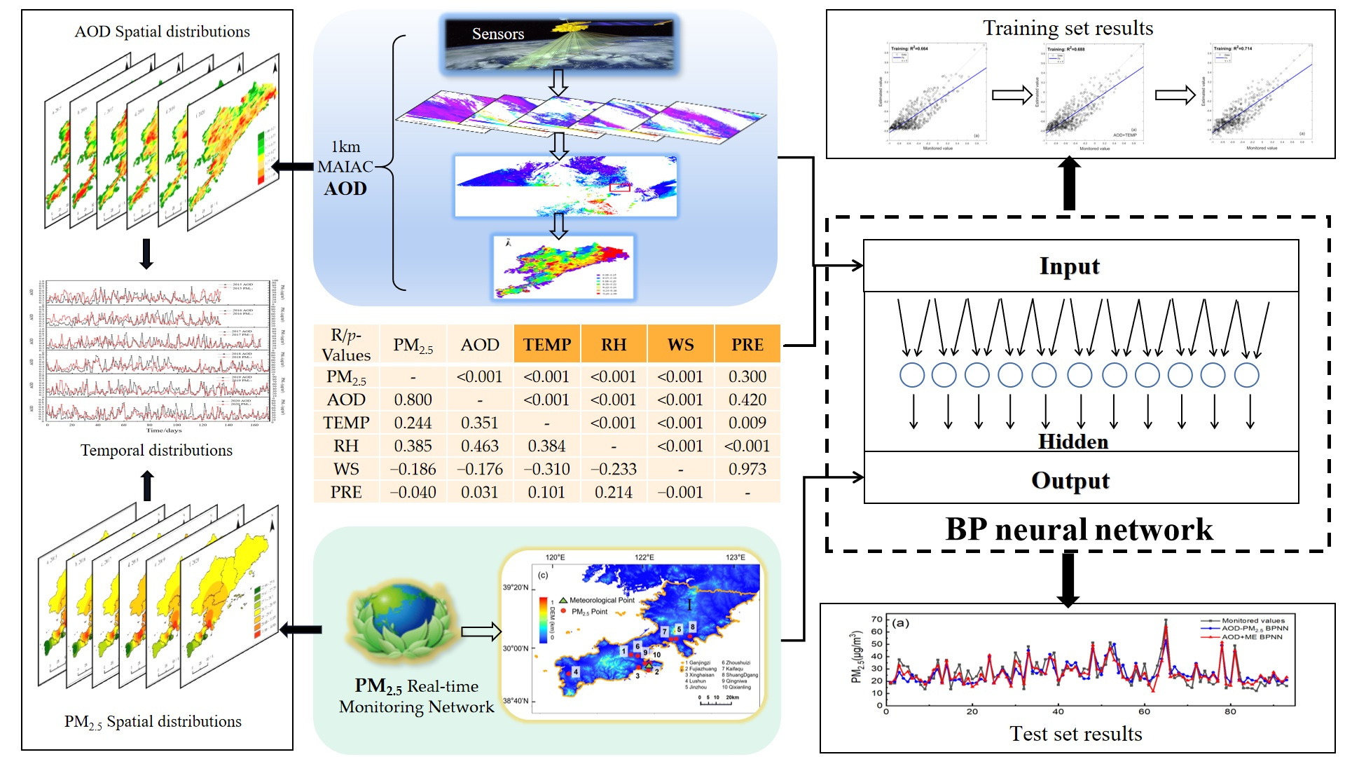
Meteorological factors affect the state and properties of particulate matter in the atmosphere, and the data are from China Meteorological network (http://data.cma.cn, accessed on 10 January 2022); this study selected the daily data of meteorological points in Figure 1c, including date, station, latitude, longitude, mean temperature (TEMP (°C)), relative humidity (RH (%)), precipitation (PRE (mm)), and average wind speed (WS (m/s)). Abundant rainfall and strong cross-ventilation are more suitable for the sedimentation and diffusion of PM2.5 particles [48]. According to the pattern exhibited by the monsoon, the aerosol solubility will be effectively diluted. The bottom-left half of Table 1 show correlation coefficient, the top-right half show p-values. There is a strong correlation between PM2.5 and AOD from Table 1. PM2.5 is positively correlated with temperature and humidity, and negatively correlated with wind speed and precipitation. In addition, the positive correlation between AOD and temperature and humidity is more significant.

2.3. Methods

2.3.1. Data Preprocessing

PM2.5 hourly mass concentration data were considered invalid if they met one of two conditions: (1) the hourly mass concentration was maintained for more than 12 h; (2) the hourly mass concentration was more than three times the standard deviation of the 24 h mass concentration [49]. The larger the aerosol AOD value, the stronger the extinction effect of aerosol on the light propagation path. The range of AOD was 0–2 (>99.4%) in this study area. According to the daily PM2.5 mass concentration and AOD data of Dalian, outliers of 8% and 9% were excluded from the box plots, respectively. The spatiotemporal distributions of annual PM2.5 concentrations were obtained through interpolation using the inverse distance weight algorithm in ArcGIS (ESRI, Redlands, CA, USA). The spatiotemporal distributions of the annual AOD data were obtained by taking the average values of daily AOD data based on ENVI.
AOD, meteorological factors, and PM2.5 were fused on the temporal–spatial scale. AOD pixels were consistent with PM2.5 measurement locations, and the AOD daily data corresponded to the PM2.5 daily data. When the AOD or PM2.5 mass concentration data were invalid for a given day, it was considered that no effective data points existed for that day. Different data fusion methods can have a great impact on correlation [50,51]. Some studies have selected typical regions to replace the whole or have used the method of taking the mean value of each region for data fusion. This study used the time series method to observe the change in the trend of AOD, meteorological factors, and PM2.5 and performed data fusion through the time series curve. AOD–meteorological factors–PM2.5 fusion data are shown in Table 2.
The dataset was divided prior to BPNN modeling. As shown in Table 3, the dataset division method of cross-dividing test sets by year was adopted, whereby each year was used as a test set to build a model, and six sub-datasets were obtained. For example, subset 6 took 2015–2019 as the training set (f) and 2020 as the test set. This type of dataset partition method compensates for the potential limitation where some data either repeatedly or do not serve as test sets and training sets due to random partition. It also eliminates the extreme error caused by random allocation of data, greatly improving the utilization rate of limited data, and can better reflect the generalization ability of the model.

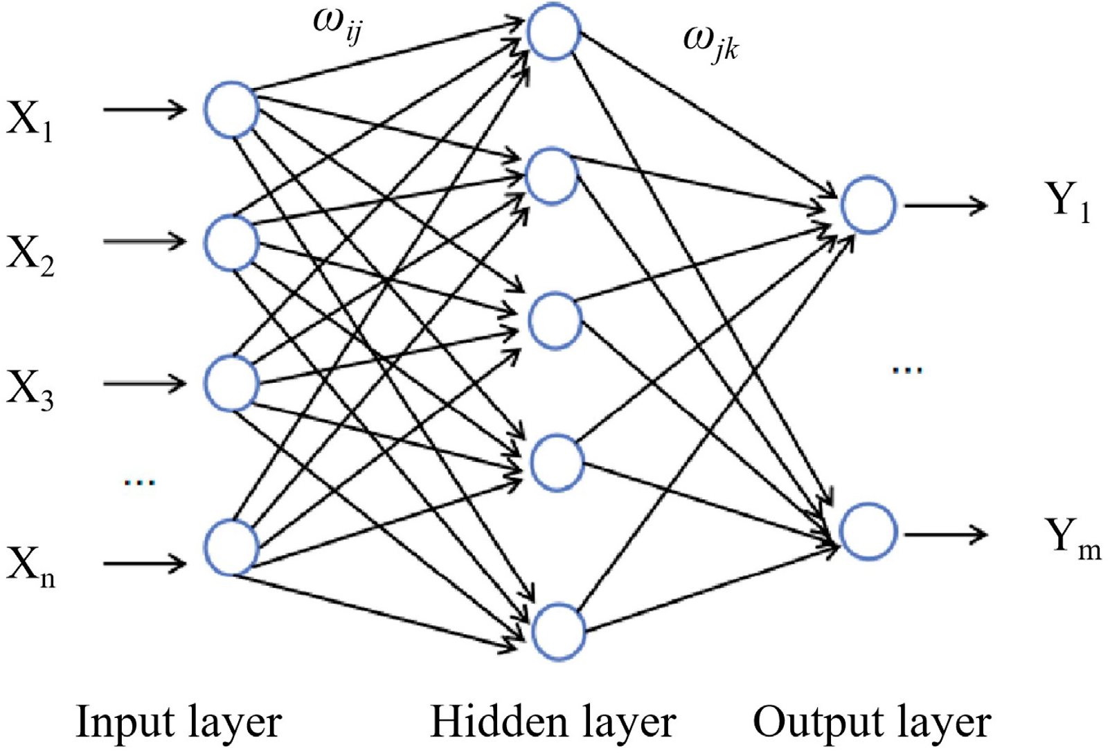
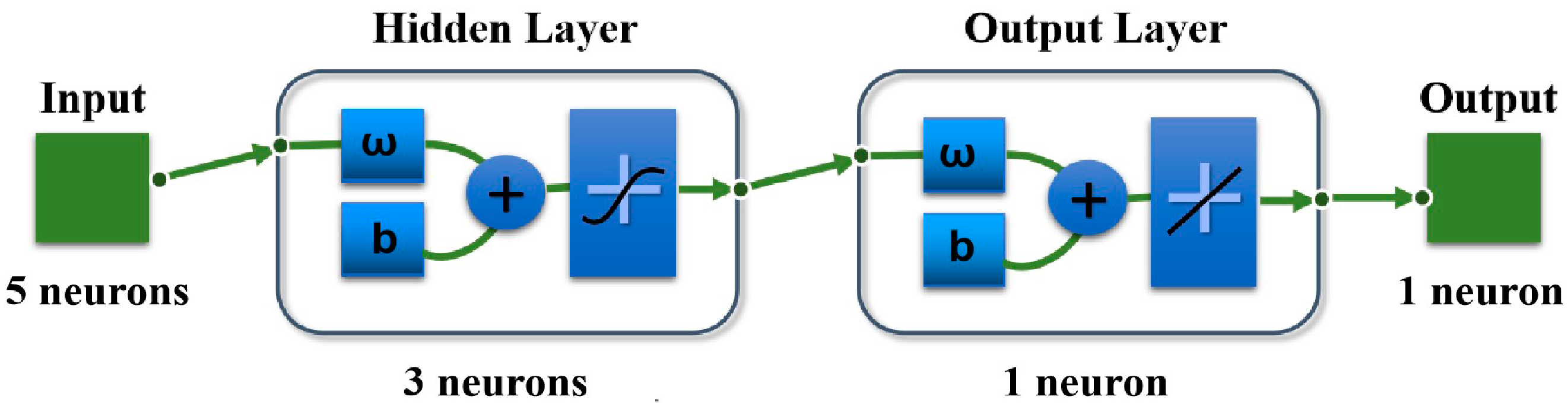
2.3.2. Establishment of BPNN

The BP algorithm is a supervised learning algorithm that utilizes the methods of mean square error and gradient descent to modify the connection weight of a network [52]. The signal enters the input layer and then enters the output layer after weighted processing and nonlinear transformation of the activation function in the hidden layer. When the error signal appears, it propagates back along the neural network, making the output value of the network close to the expected value alternately. Finally, it reaches the training result [53]. As shown in Figure 2, the structure of BPNN demonstrates that it expresses the functional mapping relationship from n independent variables to m dependent variables. x1, x2, , xn are the input of BPNN; y1, y2, , ym are the output of BPNN. In the training process of BPNN, firstly, the network should initialize the weights ωij and ωjk, initialize the thresholds aj of the hidden layer and bk of the output layer, and then calculate the hidden layer output H.
H j = f ( i = 1 n ω i j x i a j ) , j = 1 , 2 , , l
where l is the number of hidden layer neurons and f is the activation function.
Then, according to H, ωjk, and bk, BPNN prediction output O is calculated.
O k = i = 1 n H j ω j k b k , k = 1 , 2 , , m
where m is the number of output layer neurons.
According to the network prediction output O and the expected output Y, the network prediction error e is calculated.
e k = Y k O k , k = 1 , 2 , m
According to the network prediction error e, the network weight and threshold can be updated.
ω i j = ω i j + η H j ( 1 H j ) x ( i ) k = 1 m ω j k e k , j = 1 , 2 , n ; j = 1 , 2 , l
ω j k = ω j k + η H j e k , j = 1 , 2 , l ; k = 1 , 2 , , m
a j = a j + η H j ( 1 H j ) k = 1 m ω j k e k , j = 1 , 2 , l
b k = b k + η e k , k = 1 , 2 , , m
where ω′ij, ω′jk are the new weights; a′j, b′k are the new threshold, and η is the learning rate.
Iteration occurs based on the error of expected value and output value according to Formulas (1)–(7). Until the preset value reaches one of the set parameters (number of iterations, learning rate, target error), the iteration stops.
The establishment steps of BPNN in this study were divided primarily into three parts: constructing BPNN, training BPNN, and using the trained model to forecast. The steps are as follows:
Step 1: Using the newff function of MATLAB to build BPNN. According to Kolmogorov’s theorem, when the network parameters and structure design are reasonable, the neural network with a single hidden layer can complete any mapping from the n dimension to m dimension [54]. To achieve network accuracy and avoid a lengthy training time, we selected the single hidden layer neural network. As shown in Figure 3, AOD and meteorological factors were taken as the input value and PM2.5 was used as the output value to establish a BPNN.
Step 2: Determine the training parameters of BPNN. The activation function provides the BPNN with a nonlinear mapping ability. The output of the tangent S-type transfer function (tansig) is (−1, 1). If the linear transfer function (purelin) is used, the output of the whole network can be any value [55]. The tansig and purlin functions were used for the hidden layer and output layer activation function, respectively. The network training function Levenberg–Marquardt BP algorithm training function (trainlm) was selected as the network training function because it is the fastest backpropagation algorithm. In this study, combined with ten-fold cross validation, the parameters were adjusted, and the network number of iterations and learning rate were determined by the minimum error between the estimated value and the actual value. Table 4 shows the BPNN training parameters.
Step 3: Determine the number of hidden layer neurons of BPNN. The number of hidden layer neurons of BPNN has a great influence on the estimation accuracy. In this study, the number of hidden layer neurons was determined by the following empirical formula:
l = n + m + a
where l is the number of hidden layer neurons, n is the number of input layer neurons, m is the number of output layer neurons, and a is an arbitrary constant from 1 to 10 [56].
In this study, ten-fold cross validation was used to determine the network number of iterations, learning rate, and the optimal number of neurons in the hidden layer. As shown in Figure 4, the BPNN parameters corresponding to the minimum error were selected as the optimal parameters. The purpose of this process is to ensure that the BPNN is better applied to independent and unknown test sets and will eliminate the randomness of data partition of a verification set, while greatly improving the generalization ability of the model.
Step 4: Using the train function of MATLAB to train BPNN. To eliminate the error caused by variables having different magnitudes and to improve the running speed, the sample data were normalized to a data range of (−1, 1). During the training, it was ensured that the test set did not participate in the whole process.
Step 5: Using the sim function of MATLAB to simulate. The test set was input into the trained BPNN model. Due to the randomness of the initial weights and thresholds, the running results of each training were slightly different. Some of the training results were good, while others were poor. In order to evaluate the performance of the model and analyze the stability of the model, the average value of 20 running results was used as the evaluation standard of the final model.

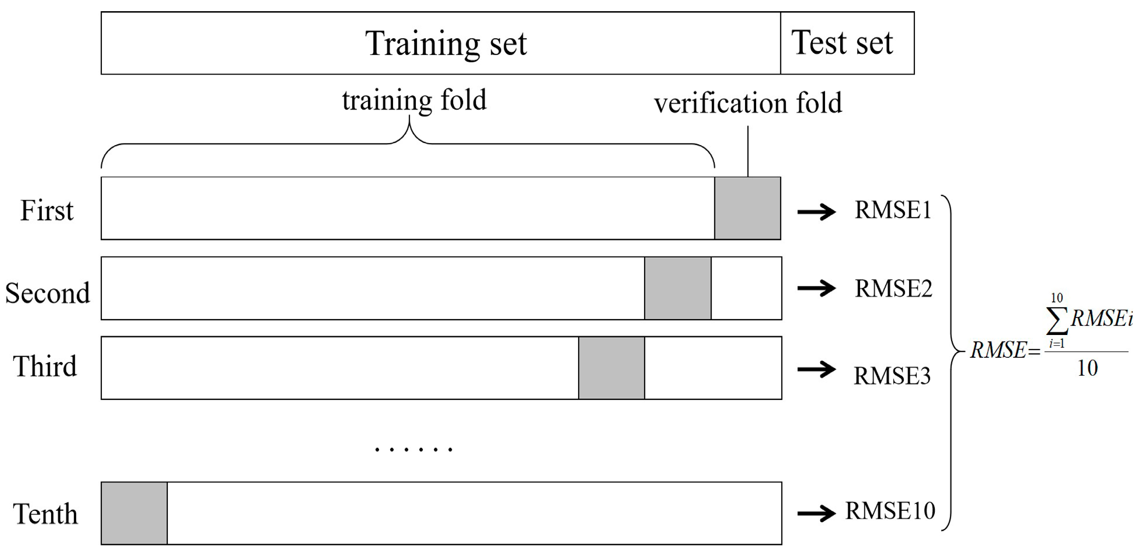
2.3.3. Model Comparison

A regression fitting model and SVR were established and compared with the BPNN. A regression analysis refers to a statistical analysis method used to determine the quantitative relationship between two or more variables, which can be divided into linear regression (LR) analysis and nonlinear regression (NLR) analysis. LR uses the best fitting straight line to establish a relationship between the dependent variable and one or more independent variables. The dependent variable of NLR is a function based on independent variables with more than one power, and the regression law is shown as a curve on the graph. Multiple regression analysis (MLR) characterizes the linear relationship between the explained variable and multiple explanatory variables. Support vector machine (SVM) and BPNN are both machine learning algorithms. SVMs are discriminative classifier techniques that convert the input space into a multi-dimensional characteristic space [57]. This method is widely used in classification and regression fields [58]. When SVM is employed for regression tasks, it is designated as an SVR [59]. The implementation of SVR in this study was based on LIBSVM (developed by Dr. Lin Chih-Jen of Taiwan University) [60]. The radial basis function (RBF) was selected as the kernel function for training. Among all the parameter pairs that enable the training set to achieve the highest verification accuracy, the best regularization parameter C and kernel function parameter gamma (g) were selected.
To compare the experimental results, 661 groups of data were divided into a training set and a test set according to the proportion of 80% and 20%. Before each model training, the datasets were reordered, and finally, the average estimate error of 20 times was obtained.

2.3.4. Correlation Evaluation Indexes

The errors of monitored values and estimated values were analyzed, as well as coefficient of determination (R2), the root mean square error (RMSE), and the prediction accuracy (Acc). The Acc formula was (9) [61]:
A c c = 1 M A P E = 1 1 n i = 1 n | P i A i | A i
where Ai was the real value data sequence, Pi was the estimated value data sequence, and n was the number of samples. MAPE was mean absolute percentage error.
The RMSE standard deviation (SD) was used to judge the stability of the model. The SD formula was (10):
S D R M S E = i = 1 n ( R M S E i R M S E ¯ ) 2 n , ( i = 1 , 2 , , n )
where n was the number of RMSE. The smaller the SDRMSE, the more stable the model.

3. Results and Discussion

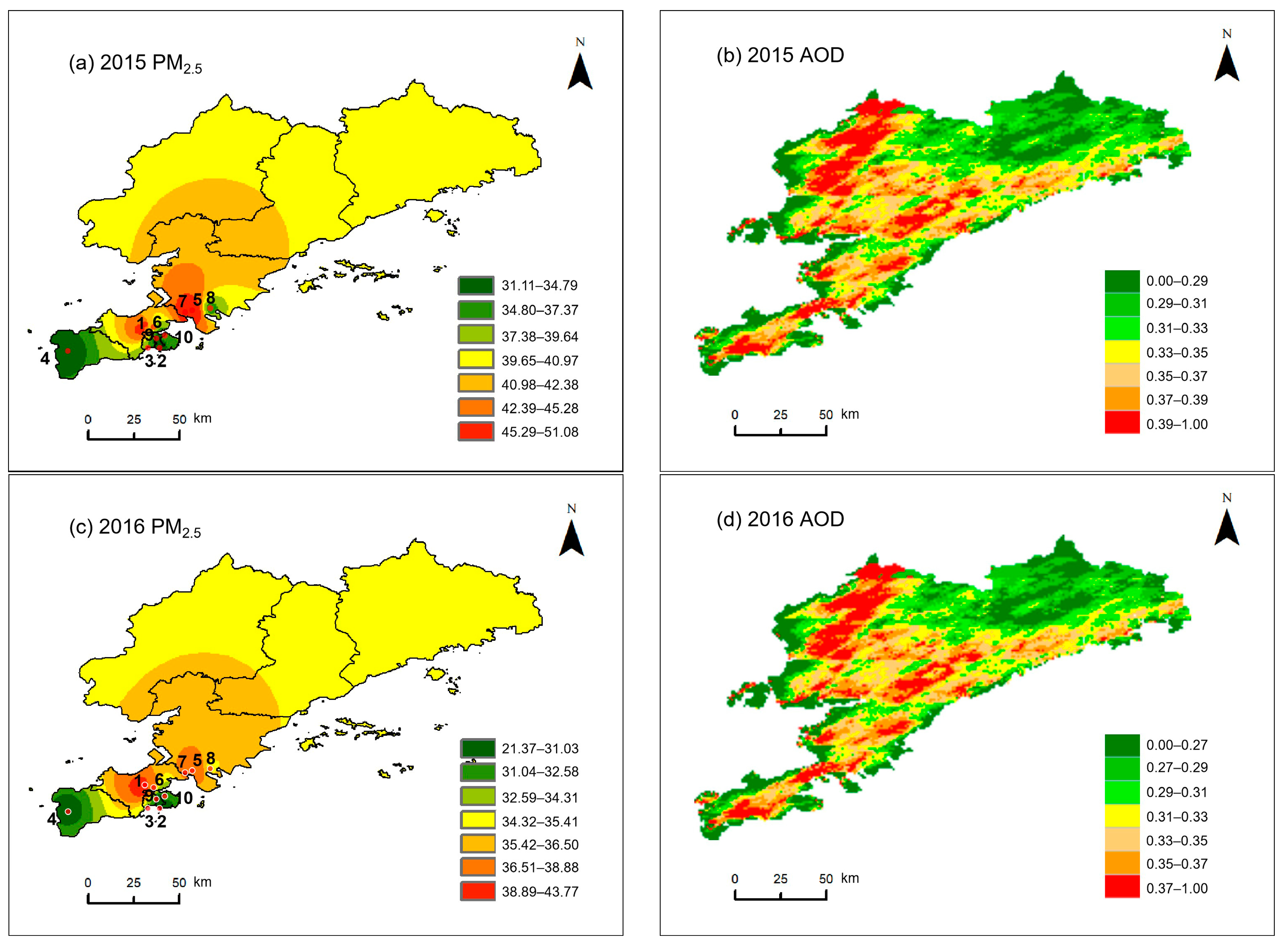
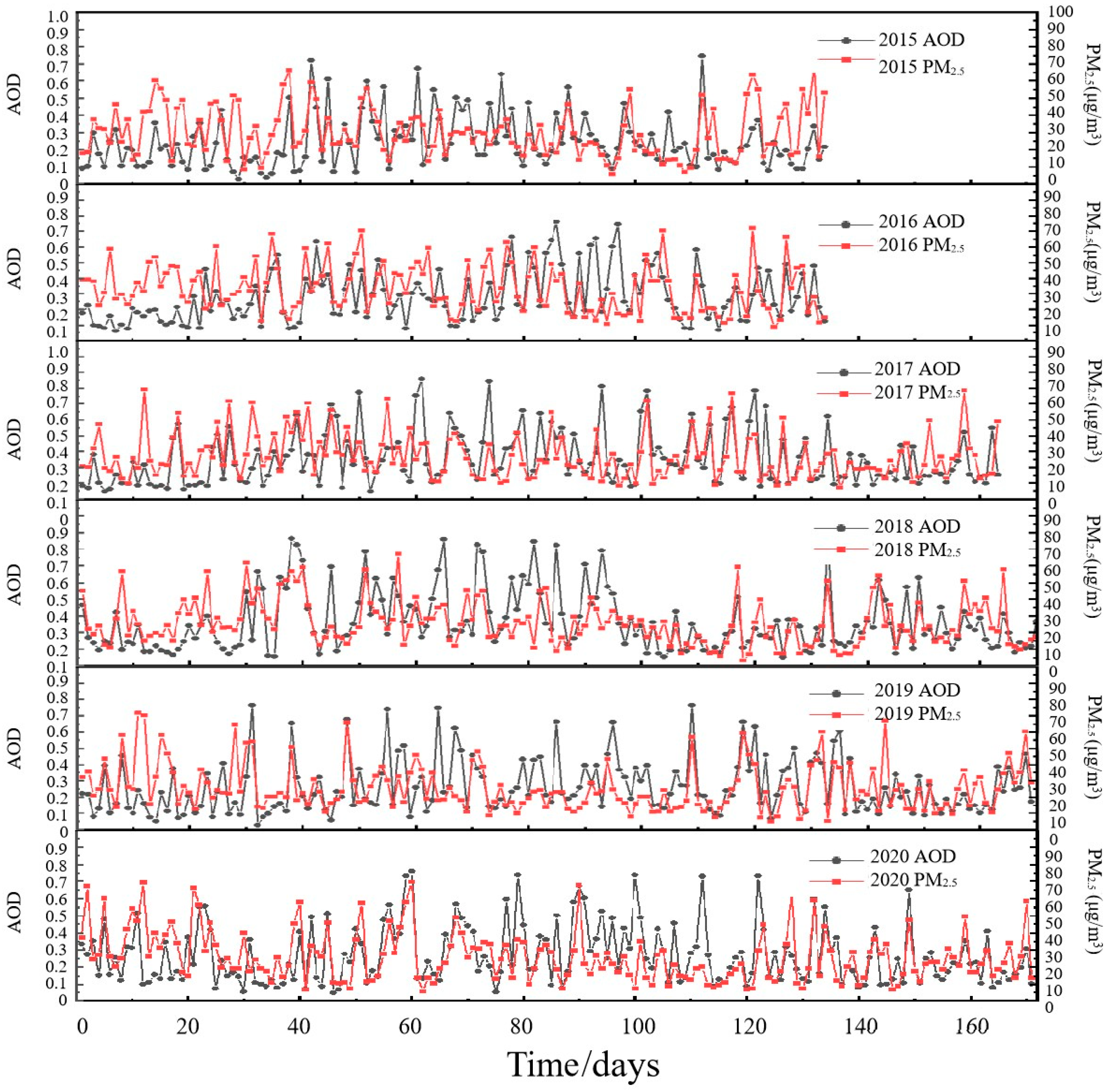
3.1. Temporal Distributions of AOD and PM2.5

The time series of AOD and PM2.5 from 2015 to 2020 are shown in Figure 5 (after eliminating outliers). The trends in AOD and PM2.5 are generally consistent, exhibiting a strong time correlation. However, there are seasonal differences: AOD was higher in summer and lower in winter, whereas the PM2.5 mass concentrations were lower in summer and autumn and higher in spring and winter.
The mean value in summer of AOD from 2015 to 2020 was 0.34, while those in the autumn and spring were 0.29 and 0.25, respectively, and it was the lowest in winter, at 0.20. In summer, Dalian has a high temperature and humidity as it is surrounded by the sea on three sides. According to the statistics in this study, the relative humidity of Dalian in summer from 2015 to 2020 was approximately 74.2%, which was 18.2% higher than that in other seasons. The high temperature and humidity environment in summer is suitable for the generation of aerosols during the transfer process of “gas–particles”, and the hygroscopic aerosols expand in humid conditions, leading to higher AOD in summer than in other seasons [62]. The AOD would be lower in winter because of lower relative humidity. The mean values of PM2.5 in summer and autumn from 2015 to 2020 were 23.9 μg/m3 and 23.5 μg/m3, respectively, while those in the spring and winter were 30.7 μg/m3 and 31.3 μg/m3, respectively. The height of the shallow boundary layer makes PM2.5 accumulate continuously in winter, resulting in higher PM2.5 concentration.
On the annual scale, AOD has obvious interannual variation characteristics. In 2015, the annual average AOD of Dalian was 0.46, which was the highest in six years. Due to the influence of pollution transportation in North China and Northeast China and local adverse meteorological factors, 2015 was the year with the heaviest particulate pollution in the six-year period. The annual mean value of AOD decreased year by year from 2016 to 2018, with a range of 0.32–0.27. In 2017, air pollution prevention and control measures, as well as dust pollution and fuel quality measures, were carried out in Dalian, resulting in a downward trend in AOD year by year. With the promotion of air pollution prevention and a control action plan, the annual mean value of AOD in 2019 and 2020 tended to be stable, and the value remained at 0.27.

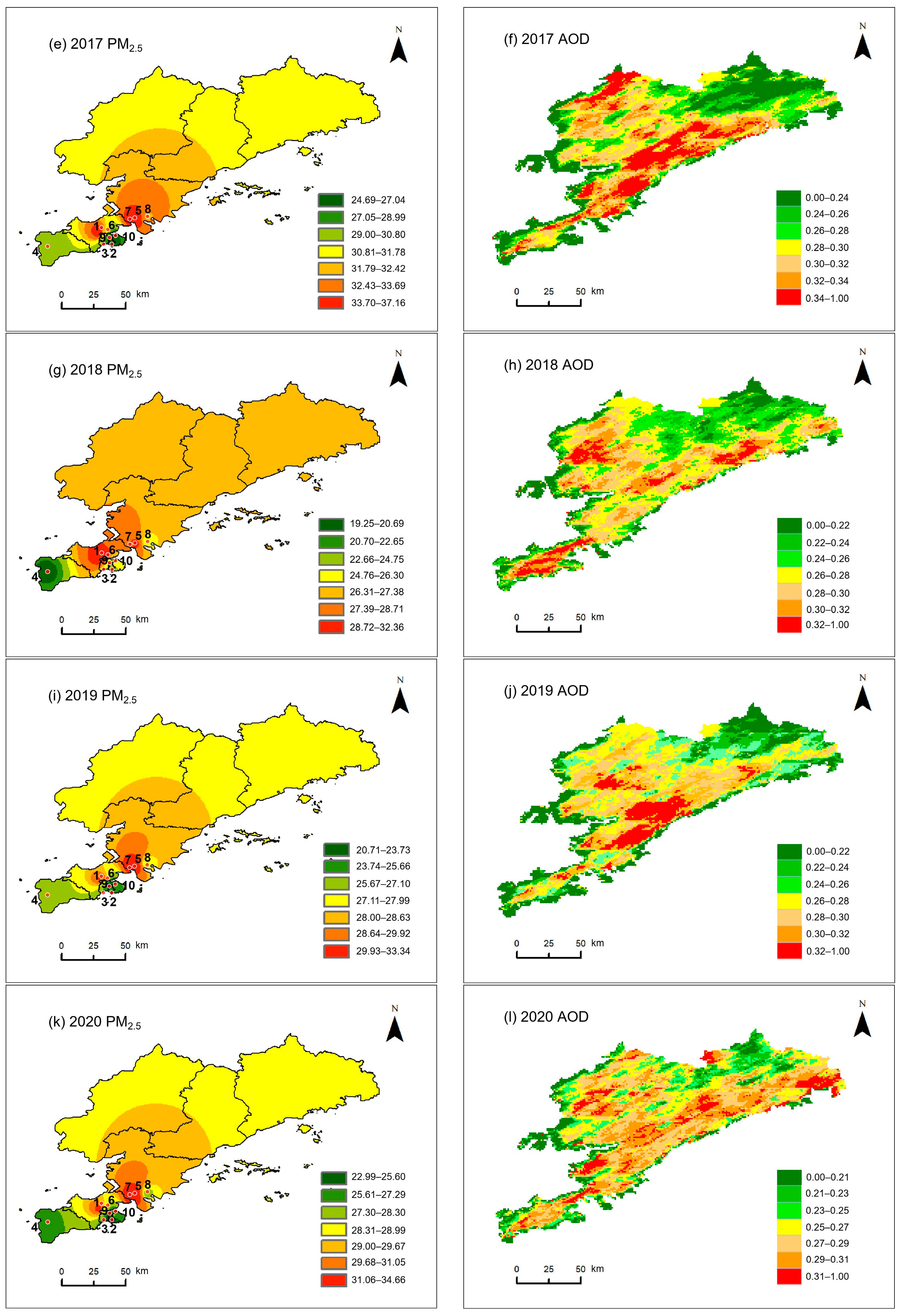
3.2. Spatial Distributions of AOD and PM2.5
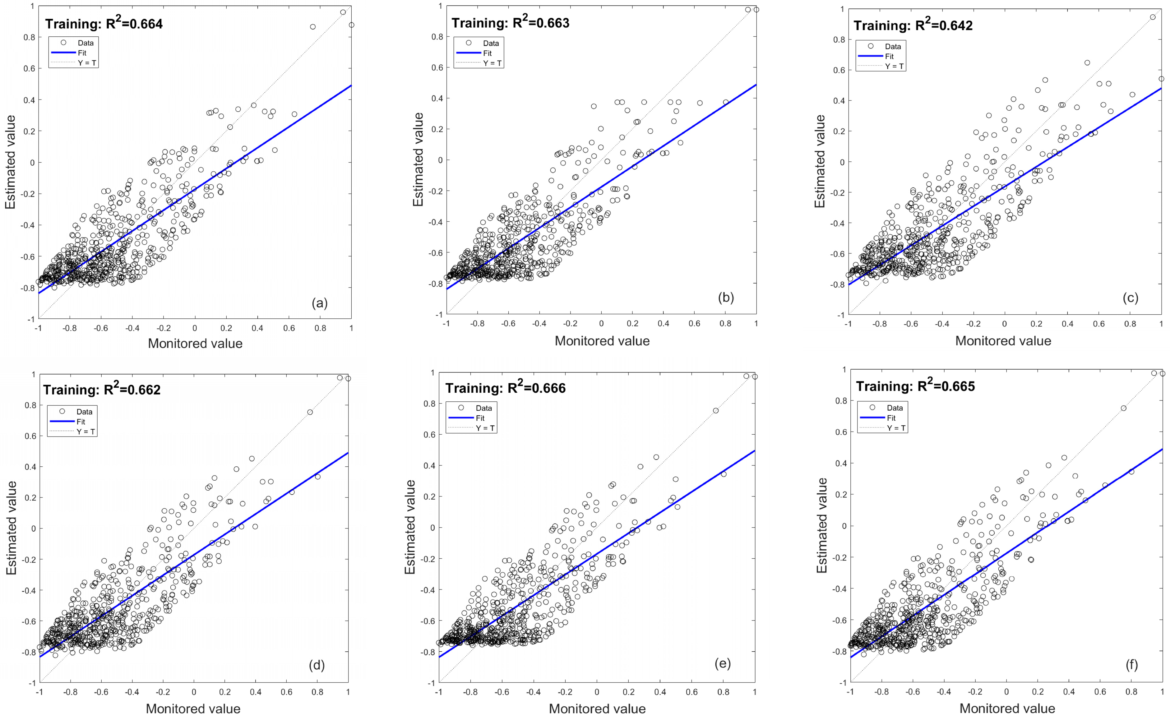
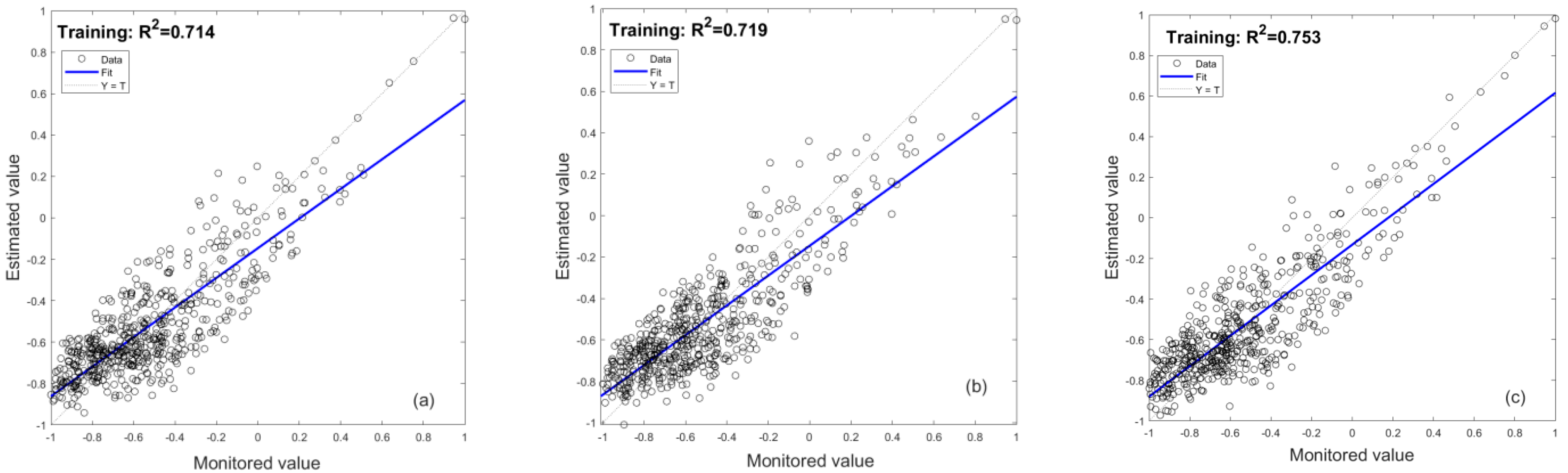
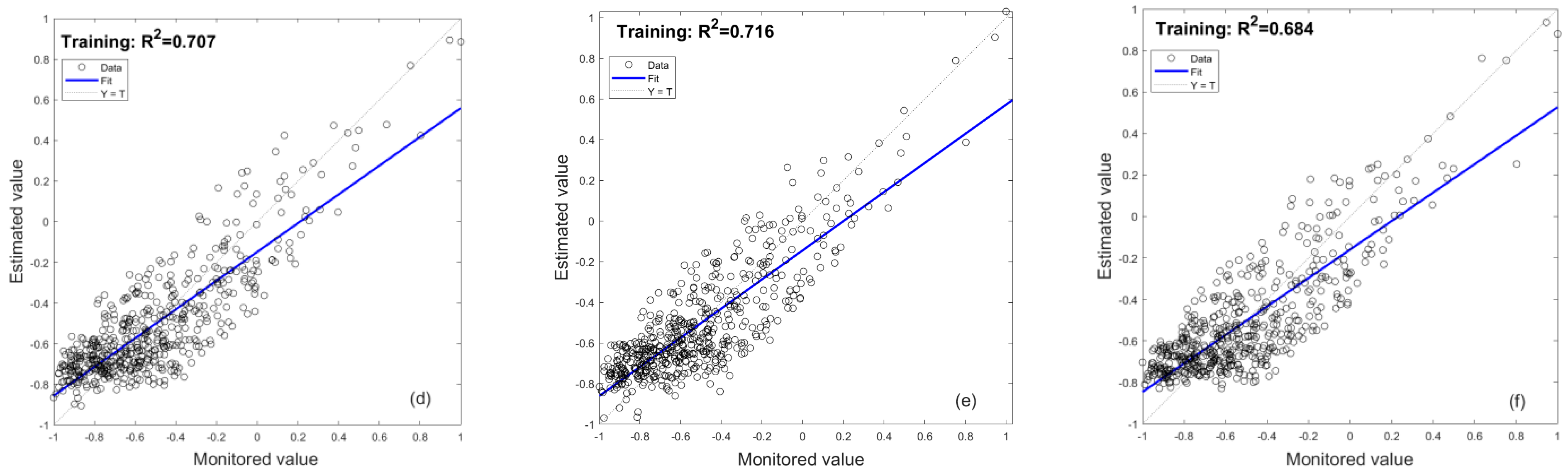
As shown in Figure 6, there was a high value region of PM2.5 and AOD concentrations in the southwest of Dalian, wherein smoke and dust are produced by industrial processes and exhaust fumes are emitted by vehicles. The average concentrations of PM2.5 in monitoring points 1 and 6 were 37.06 and 33.69 μg/m3, respectively. The PM2.5 concentrations of the coastal areas were relatively low, with monitoring points 2, 4, 9, and 10 showing average PM2.5 concentrations of 26.42, 27.33, 25.76, and 28.62 μg/m3, respectively. The average AOD values in monitoring points 1 and 6 were 0.32 and 0.29, respectively. Monitoring points 2, 4, 9, and 10 had a relatively low AOD, with mean AOD values of 0.21, 0.24, 0.22, and 0.22, respectively. From the perspective of the whole region of Dalian, northeastern Dalian had a low average AOD of 0.24, and the average AOD in the main urban area was 0.33. The spatiotemporal distribution of AOD and PM2.5 demonstrated good correlation as their extreme points were consistent (R2 = 0.922) with the high values in the main urban area and low values in the northern urban–rural area.
The AOD overall spatial distribution of the remote sensing can be obtained from Figure 6. The AOD value in the northeastern part of Dalian is relatively low, while the AOD value in the northwestern part and the eastern coastal area is relatively high. The distribution curve of Dalian’s population density (https://www.worldpop.org/, accessed on 10 January 2022) in 2020 and the spatial structure of Dalian are shown in Figure 7. PM2.5 and AOD had high values in areas with a high population density, and low values in Zhuanghe City, North Dalian, where the population density was relatively low. Jinzhou District and Pulandian District in central Dalian had a moderate population density, and PM2.5 and AOD were also widely distributed in this area. There is a core and two wings in the spatial structure of Dalian, which takes the city center as the core and takes the developments along the Bohai Sea and the Yellow Sea. Seven sub-center cities of Dalian are connected with industrial groups. Wafangdian City is in the northwest geographically, where there are three industrial nodes. AOD values are high, the same as the eastern seaboard. Therefore, population density, industrial layout, and urban planning have a certain impact on the distribution of PM2.5 and AOD.

3.3. BPNN

BPNN was trained through adjusting the parameters according to the step length. In the iterative process of data calculation, the parameters take values at a certain interval, and this interval is called the step length, which should be determined according to the amount of data and the complexity of the algorithm. This study took 500 as the step length and set the number of iterations from 500 to 5000 by experiments. The value of the learning rate is between (0,1). We choose the learning rate as 0.1, 0.2, 0.3.... for training, respectively. The target error is determined based on the magnitude of the data and the actual accuracy of the model when it is training. After ten-fold cross-training, the average RMSE of training sets (a) to (f) in terms of the number of iterations and learning rate were 6.48 μg/m3–6.82 μg/m3 and 6.38 μg/m3–7.23 μg/m3, respectively. When the number of iterations and learning rate were 3000 and 0.1, respectively, the RMSE was the smallest.
According to Formula (8), the number of neurons in the hidden layer of BPNN was determined to be between 2 and 12. After ten-fold cross-training, the average value of the RMSE of the verification set corresponding to the number of hidden layer neurons was obtained. The results of ten-fold cross-verification of training sets (a) to (f) are shown in Table 5. Compared with the number of iterations and learning rate, the selection of the number of hidden layer neurons has a great influence on the estimation accuracy, and the optimal hidden layer neurons of the six BPNN models (RMSEa–f) were determined to be 3, 2, 2, 2, 3, and 2, respectively.
According to the above settings, the BPNN was trained with the error gradually approximated from the target error. The prediction results of the BPNN training set (a)–(f) with AOD as a single input variable are shown in Figure 8, and the scale is PM2.5 normalized value. The R2 value between the estimated values and the monitored value of the training set (a)–(f) were about 0.660. However, there is a positive offset and a small slope, which means that there is underestimation for high value or overestimation for low value in the forecast time series. Therefore, any of the cases selected in Figure 8 were introduced with the meteorological factors for the training set, respectively, with set (a) as an example, and the prediction results are shown in Figure 9. The specific R2 values increasing were, respectively, 0.024, 0.023, 0.01, and 0.008, corresponding to TEMP, RH, PRE, and WS, and the positive offsets were also improved.
Four meteorological factors and AOD were considered as input, and the prediction results of the BPNN training set are shown in Figure 10. From the comparison between Figure 8 and Figure 10, it can be seen that the R2 value in each case was increased about 0.055, and the maximum value was increased by 0.111. In addition, the positive offset was improved significantly. Meteorological factors can improve the estimation accuracy of the model and have an important impact on the estimation of PM2.5.
The test sets were input into the trained BPNN. After 20 runs, the R2 and RMSE of the estimated PM2.5 values and the monitored value were calculated and are shown in Table 6. The range of R2 values were 0.663–0.752 and the range of RMSE values were 6.23–6.45 μg/m3. The R2 value in each case was increased by about 0.032, and the maximum value was increased by 0.046. Temperature had the greatest impact on model accuracy among meteorological factors. In addition, the RMSE SD values were 0.01–0.05 μg/m3. These findings indicate that the model has a strong generalization ability and stability, which is close to the simulation effect of the training set; hence, there was no overfitting.
Figure 11 is the simulation diagram of the last running results of six models with 2015–2020 as the test set. The estimation result of the BPNN with the introduction of meteorological factors is better than that of the AOD–PM2.5 BPNN. However, it can be seen from Figure 11d that the model has not yet reached the estimation of PM2.5 for lower concentrations. That is to say, the BPNN model can be used to estimate the trend of interannual PM2.5 and needs to be improved for estimating the daily extreme value of PM2.5 in the future.

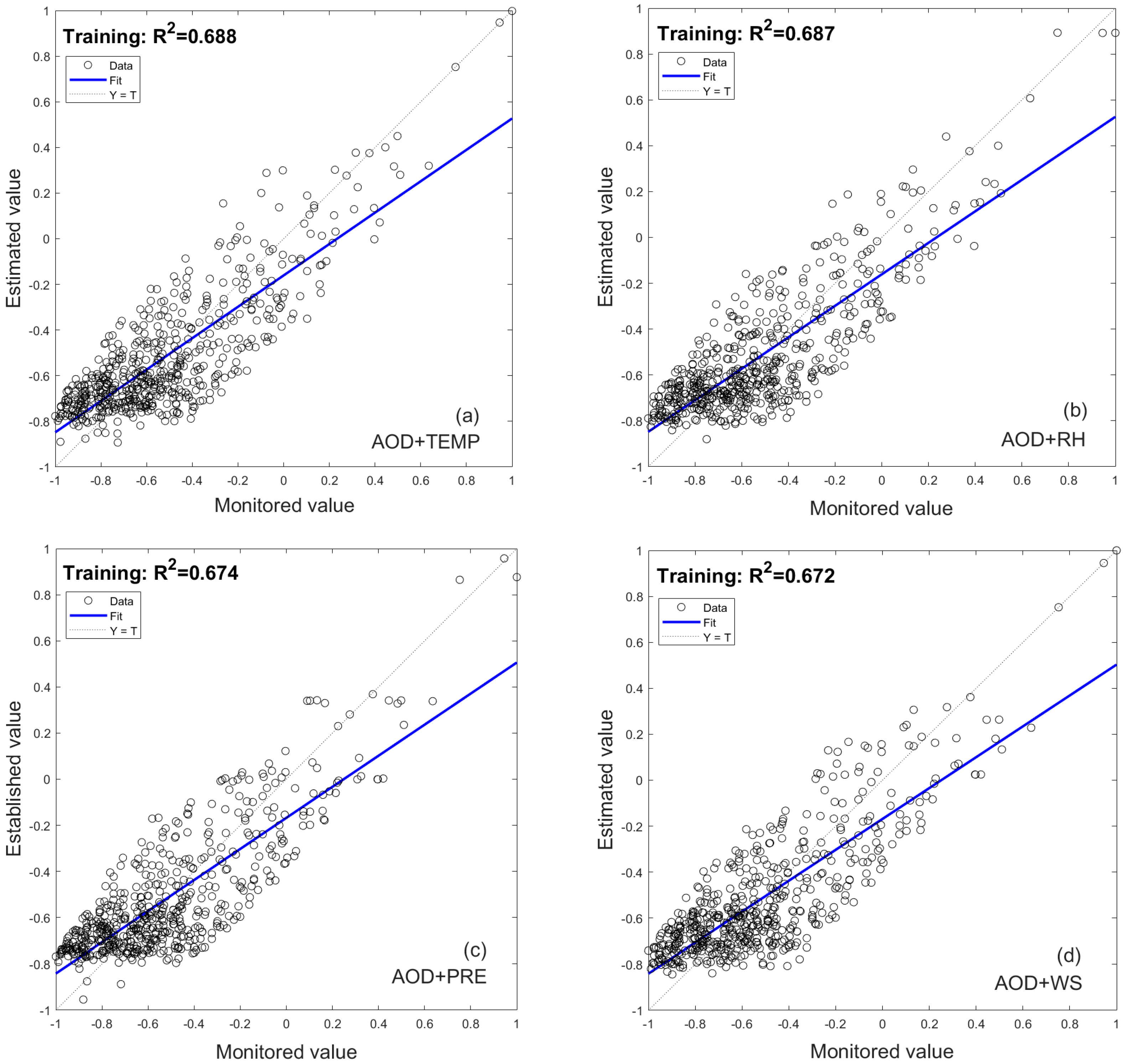
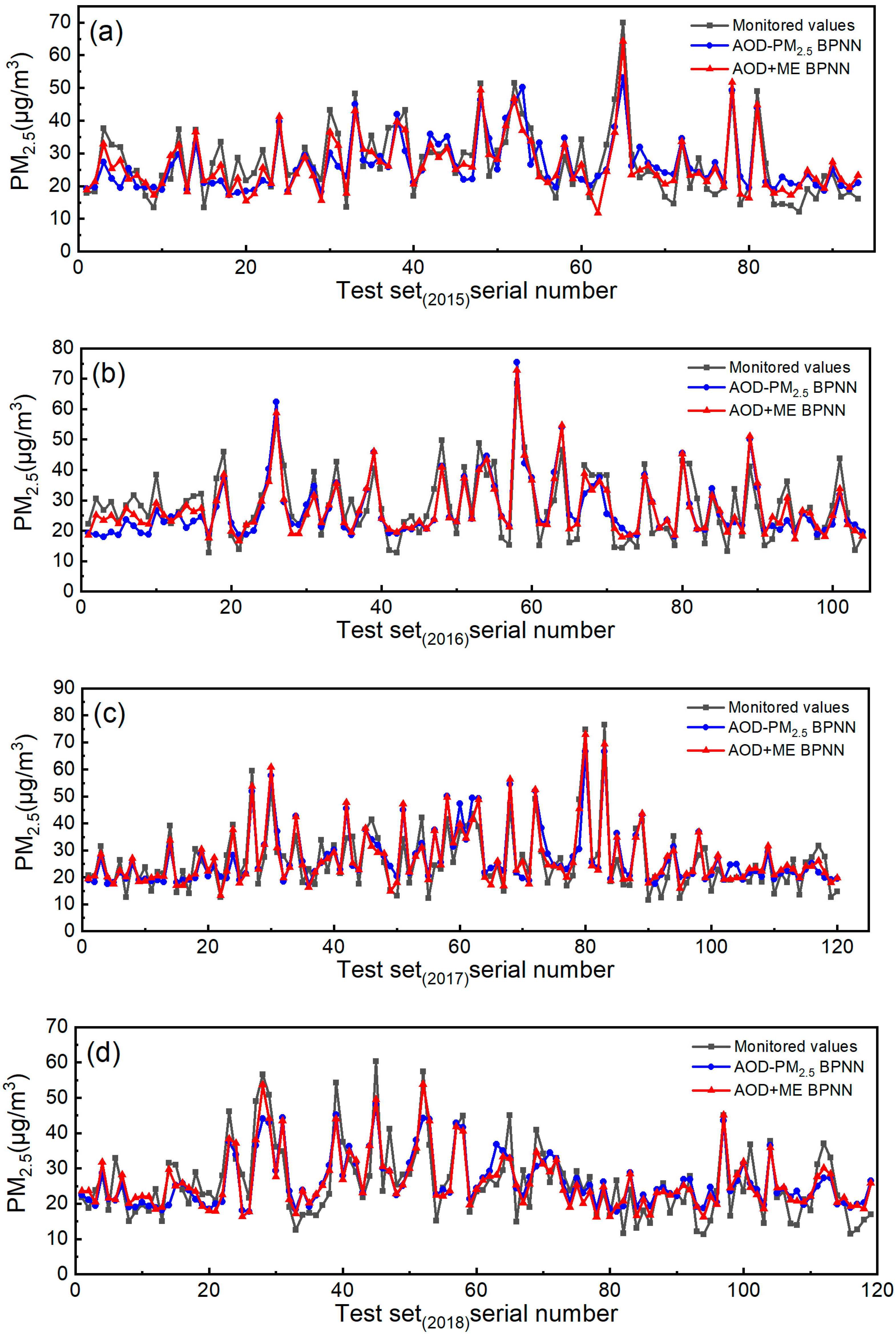
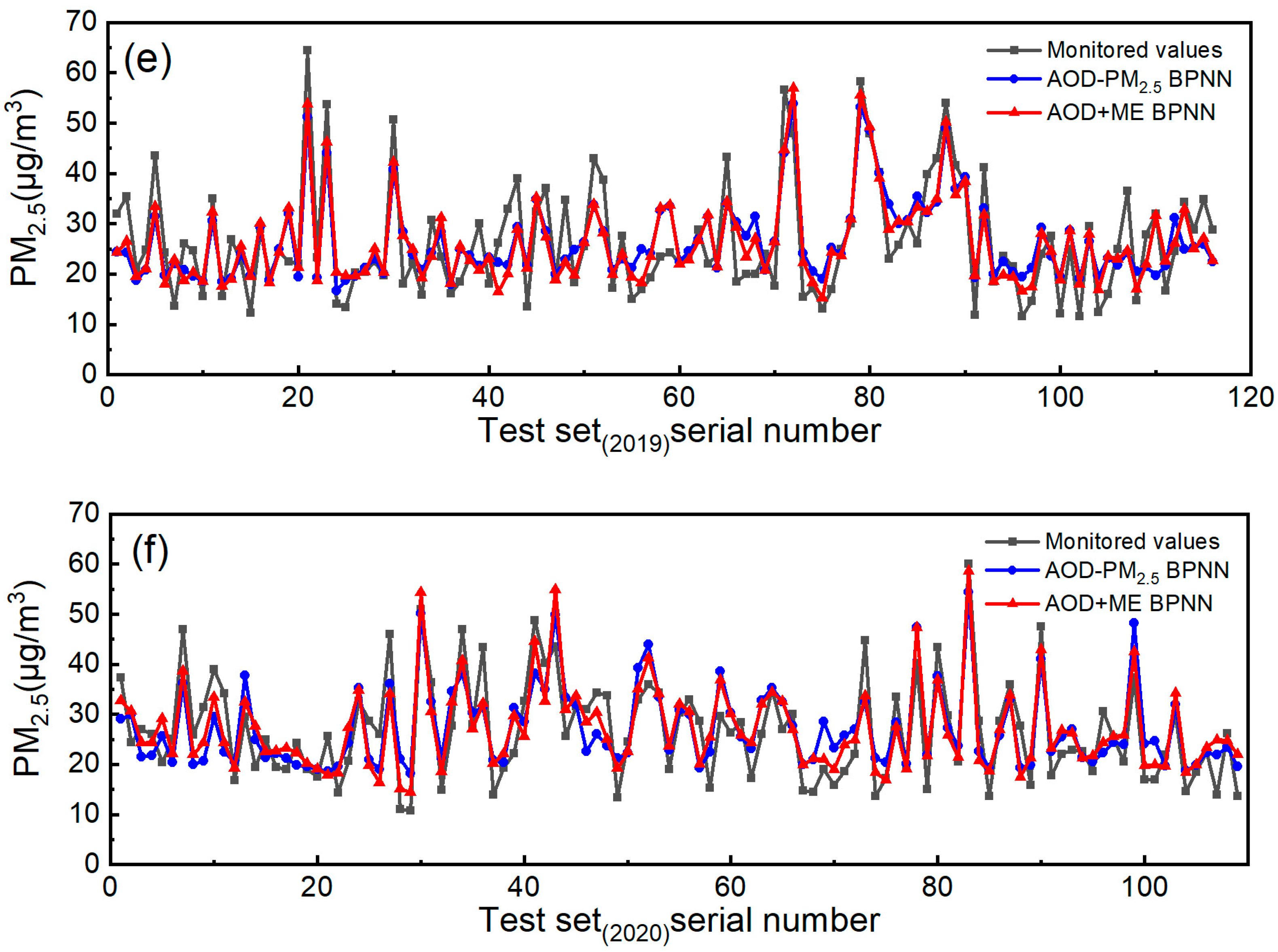
3.4. Comparison of BPNN with Regression Analysis and SVR

The parameters and average error results of the last operation of BPNN, LR, NLR, MLR, and SVR are shown in Table 7. The R2 values of all models were all above 0.650, and the precision of meteorological factors–BPNN was the highest, with an R2 of 0.757 and an RMSE of 6.11 μg/m3. Compared with the LR, NLR, MLR, and SVR methods, the R2 and RMSE of BPNN were improved; however, the improvement degree was not significant. According to the comparison results, the regression equation obtained by the regression analysis model is relatively intuitive. Under the influence of structure, BPNN cannot directly showcase the direct correlation between output and input, but the neural network stores information in the connection weight. When the error between the expected and output reaches the requirement, the corresponding relationship of input and output can be obtained. LR, MLR, and NLR curves can only describe the approximate relationship between variables; the complicated regression cannot reflect the relationship among all regression data. The optimal nonlinear model obtained in this study was a univariate cubic model, but it was not determined whether it described the essential relationship between variables. BPNN approaches the objective function by learning, and a single hidden layer can be used to fit complex and continuous functions; hence, the computational sophistication of BPNN is reduced. The results showed that the accuracy of BPNN was similar to that of SVR, but SVR ran for a long time. Therefore, BPNN is superior to other models used in this study in terms of the PM2.5 concentration estimate.

3.5. Discussion

3.5.1. Research Findings

To date, relevant studies have primarily focused on PM2.5 inversions based on satellite remote sensing data. Statistical models (e.g., linear mixed models, geographically weighted regressions, and geographically and temporally weighted regressions) are commonly used for this purpose, all delivering high R2 values (0.64–0.86) [63,64,65]. We analyzed the spatiotemporal correlation between AOD and PM2.5 and performed simple regression fitting. We determined that a simple linear relationship between AOD and PM2.5 did not exist, which made it difficult to accurately model using traditional regression methods. In this case, we established a BPNN with a strong nonlinear description ability. Mathematically, it was proven that the three-layer neural network could approach any nonlinear continuous function with arbitrary precision, which was further confirmed by the research results of the current study. Regarding the overfitting, underfitting, and sample dependence problems of BPNN, we made improvements in three aspects, namely, dataset division, model parameter determination, and model evaluation, which compensated for the deficiencies of the BPNN. The space–time extra trees (STET) were about 0.8, which were higher than those of BPNN (R2 = 0.66–0.75) in recent studies [66,67], and the R2 of MLR was reduced to 0.54 in some time or regions. Both of them had poor stability. The BPNN prediction model had great temporal and spatial consistency and was more suitable for universal prediction. Significantly, the RMSE (6.36 μg/m3) mean of the BPNN was much lower than MLR (7.18 μg/m3, 13.4 μg/m3) and STET (14.60 μg/m3), which proved that BPNN was advantageous in estimating the AOD of PM2.5. Prior studies focused on the correlation between PM2.5 and AOD spatiotemporal distribution or established a model to estimate PM2.5 [68,69,70]. This study analyzed the correlation between MAIAC AOD and PM2.5 in terms of seasonal scale, spatial scale, and annual scale, as well as established an estimation model to provide a theoretical reference for variations in the characteristics of AOD and PM2.5.

3.5.2. Limitations

Although applying the BPNN to estimate PM2.5 based on AOD has research merit, this approach also has certain limitations.
(1)
Here, the limited number of ground measurement points impeded the analysis of the spatiotemporal correlations between AOD and PM2.5.
(2)
Seasonal differences in AOD and PM2.5 were not incorporated into the establishment of BPNN.
(3)
The BPNN model can be used to estimate the trend of interannual PM2.5 and needs to be improved for estimating the daily extreme value of PM2.5 in the future.
Subsequent research should focus on more PM2.5 and AOD historical data, data on daily to hourly timescales, and investigation of spatiotemporal characteristics. At the same time, future research should expand the scope of model comparison and explore the advantages of machine learning.

4. Conclusions

PM2.5 is the most important pollutant in the atmosphere, and it not only affects the ecological environment, but also endangers human health. AOD is an important index to evaluate the change in atmospheric environment. In this study, AOD was used to estimate the mass concentration of PM2.5 in order to realize the full space coverage of PM2.5, which is crucial for air quality monitoring and human health research. Therefore, based on the analysis of spatiotemporal correlation, a BPNN model with joint cross-validation was established to accurately estimate the daily concentration of PM2.5 in Dalian, China. MAIAC AOD and PM2.5 exhibited strong spatiotemporal correlations. Temporally, AOD was higher in summer and lower in winter, whereas PM2.5 mass concentrations were lower in summer and autumn and higher in spring and winter. On the annual scale, the AOD of Dalian showed a decreasing trend, year by year. Spatially, the spatiotemporal distribution of AOD and PM2.5 demonstrated a good correlation (R2 = 0.922), and this result was consistent with the distribution of population density. In this study, each year from 2015 to 2020 was used as the test set, and other years were used as the training set. Using AOD and meteorological factors (TEMP, WS, RH, PRE) as the input of the model, six BPNN models were established. The results showed that the estimation result of the BPNN with the introduction of meteorological factors is better than that of the AOD–PM2.5 BPNN. The range of R2 values were 0.663–0.752 and the range of RMSE values were 6.23–6.45 μg/m3. The R2 value in each case was increased by about 0.032. Temperature had the greatest impact on model accuracy among meteorological factors. The difference caused by the randomness of the initial weight and threshold of BPNN to the operation results of the model was considered. We further compared the performance of BPNN with regression models and SVR. The results demonstrated that BPNN was advantageous over the LR, NLR, MLR, and SVR methods in terms of the model sophistication and training time. Therefore, BPNN with a generalization ability and stability can be considered as the best candidate technology for PM2.5 concentration estimation, providing scientific basis for macroscopic and long-term monitoring of air pollution.

Author Contributions

Conceptualization, J.G., X.L., and Y.W.; methodology, data curation, formal analysis, investigation, and writing—original draft preparation, Y.W., J.M., and Y.L.; writing—review and editing, supervision, J.G. and S.W. All authors have read and agreed to the published version of the manuscript.

Funding

This research study was supported by the National Natural Science Foundation of China (grant no. 41671158, 41771178) and supported by Foundation of Liaoning Educational Committee (LJKZ0979).

Institutional Review Board Statement

Not applicable.

Informed Consent Statement

Not applicable.

Data Availability Statement

The data that support the findings of this study are available from the corresponding author, upon reasonable request.

Acknowledgments

We appreciate the data provided by National PM2.5 Real-time Monitoring Network (http://www.pm25china.net, accessed on 10 January 2022), Level-1 and the Atmosphere Archive and Distribution System Distributed Active Archive Center (https://ladsweb.modaps.eosdis.nasa.gov/, accessed on 10 January 2022) and China Meteorological network (http://data.cma.cn, accessed on 10 January 2022).

Conflicts of Interest

The authors declare no conflict of interest.

References

  1. Pope, C.A., III. Lung Cancer, Cardiopulmonary Mortality, and Long-term Exposure to Fine Particulate Air Pollution. JAMA 2002, 287, 1132. [Google Scholar] [CrossRef] [PubMed] [Green Version]
  2. Song, Y.M.; Huang, B.; He, Q.Q.; Chen, B.; Wei, J.; Mahmood, R. Dynamic assessment of PM2.5 exposure and health risk using remote sensing and geo-spatial big data. Environ. Pollut. 2019, 253, 288–296. [Google Scholar] [CrossRef] [PubMed]
  3. Lim, C.C.; Hayes, R.B.; Ahn, J.; Shao, Y.; Silverman, D.T.; Jones, R.R.; Garcia, C.; Thurston, G.D. Association between long-term exposure to ambient air pollution and diabetes mortality in the US. Environ. Res. 2018, 165, 330–336. [Google Scholar] [CrossRef]
  4. Liu, M.; Tang, W.; Zhang, Y.; Wang, Y.; Kangzhuo, B.; Li, Y.; Liu, X.; Xu, S.; Ao, L.; Wang, Q.; et al. Urban-rural differences in the association between long-term exposure to ambient air pollution and obesity in China. Environ. Res. 2021, 201, 111597. [Google Scholar] [CrossRef]
  5. Liu, Y.P.; Wu, J.G.; Yu, D.Y.; Hao, R.F. Understanding the Patterns and Drivers of Air Pollution on Multiple Time Scales: The Case of Northern China. Environ. Manag. 2018, 61, 1048–1061. [Google Scholar] [CrossRef]
  6. Liu, J.J.; Weng, F.Z.; Li, Z.Q.; Cribb, M.C. Hourly PM2.5 Estimates from a Geostationary Satellite Based on an Ensemble Learning Algorithm and Their Spatiotemporal Patterns over Central East China. Remote Sens. 2019, 11, 2120. [Google Scholar] [CrossRef] [Green Version]
  7. Li, L.F. A Robust Deep Learning Approach for Spatiotemporal Estimation of Satellite AOD and PM2.5. Remote Sens. 2020, 12, 264. [Google Scholar] [CrossRef] [Green Version]
  8. Han, X.; Cui, X.; Ding, L.; Li, Z. Establishment of PM2.5 Prediction Model Based on Maiac AOD Data of High Resolution Remote Sensing Images. Int. J. Pattern Recognit. 2019, 33, 1954009. [Google Scholar] [CrossRef]
  9. Fu, D.; Song, Z.; Zhang, X.; Wu, Y.; Duan, M.; Pu, W.; Ma, Z.; Quan, W.; Zhou, H.; Che, H.; et al. Similarities and Differences in the Temporal Variability of PM2.5 and AOD between Urban and Rural Stations in Beijing. Remote Sens. 2020, 12, 1193. [Google Scholar] [CrossRef] [Green Version]
  10. Xue, W.H.; Zhang, J.; Zhong, C.; Ji, D.Y.; Huang, W. Satellite-derived spatiotemporal PM2.5 concentrations and variations from 2006 to 2017 in China. Sci. Total Environ. 2020, 712, 77–144. [Google Scholar] [CrossRef]
  11. Wei, J.; Peng, Y.R.; Mahmood, R.; Sun, L.; Guo, J.P. Intercomparison in spatial distributions and temporal trends derived from multi-source satellite aerosol products. Atmos. Chem. Phys. 2019, 19, 7183–7207. [Google Scholar] [CrossRef] [Green Version]
  12. Levy, R.C.; Mattoo, S.; Munchak, L.A.; Remer, L.A.; Sayer, A.M.; Patadia, F.; Hsu, N.C. The Collection 6 MODIS aerosol products over land and ocean. Atmos. Meas. Tech. 2013, 6, 2989–3034. [Google Scholar] [CrossRef] [Green Version]
  13. Hsu, N.C.; Jeong, M.-J.; Bettenhausen, C.; Sayer, A.M.; Hansell, R.; Seftor, C.S.; Huang, J.; Tsay, S.-C. Enhanced Deep Blue aerosol retrieval algorithm: The second generation. J. Geophys. Res. Atmos. 2013, 118, 9296–9315. [Google Scholar] [CrossRef]
  14. Nabavi, S.O.; Haimberger, L.; Abbasi, E. Assessing PM2.5 concentrations in Tehran, Iran, from space using MAIAC, deep blue, and dark target AOD and machine learning algorithms. Atmos. Pollut. Res. 2019, 10, 889–903. [Google Scholar] [CrossRef]
  15. Fu, H.C.; Sun, Y.L.; Chen, L.; Zhang, H.; Gao, S. Temporal and spatial distribution characteristics of PM2.5 and PM10 in Xinjiang region in 2016 based on AOD data and GWR model. Acta Sci. Circumstantiae 2020, 40, 27–35. [Google Scholar]
  16. Ahmad, M.; Alam, K.; Tariq, S.; Anwar, S.; Mansha, M. Estimating fine particulate concentration using a combined approach of linear regression and artificial neural network. Atmos. Environ. 2019, 219, 117050. [Google Scholar] [CrossRef]
  17. Shen, X.; Bilal, M.; Qiu, Z.; Sun, D.; Wang, S.; Zhu, W. Validation of MODIS C6 Dark Target Aerosol Products at 3 km and 10 km Spatial Resolutions over the China Seas and the Eastern Indian Ocean. Remote Sens. 2018, 10, 573. [Google Scholar] [CrossRef] [Green Version]
  18. Bilal, M.; Nichol, J.; Spak, S. A New Approach for Estimation of Fine Particulate Concentrations Using Satellite Aerosol Optical Depth and Binning of Meteorological Variables. Aerosol. Air Qual. Res. 2017, 11, 356–367. [Google Scholar] [CrossRef] [Green Version]
  19. Zhang, J.; Xin, J.; Zhang, W.; Wang, S.; Wang, L.; Xie, W.; Xiao, G.; Pan, H.; Kong, L. Validation of MODIS C6 AOD products retrieved by the Dark Target method in the Beijing–Tianjin–Hebei urban agglomeration, China. Adv. Atmos. Sci. 2017, 34, 993–1002. [Google Scholar] [CrossRef]
  20. Xie, G.Q.; Wang, M.; Pan, J.; Zhu, Y. Spatio-temporal variations and trends of MODIS C6.1 Dark Target and Deep Blue merged aerosol optical depth over China during 2000–2017. Atmos. Environ. 2019, 214, 46–76. [Google Scholar] [CrossRef]
  21. Jethva, H.; Torres, O.; Yoshida, Y. Accuracy assessment of MODIS land aerosol optical thickness algorithms using AERONET measurements over North America. Atmos. Meas. Tech. 2019, 12, 4291–4307. [Google Scholar] [CrossRef] [Green Version]
  22. Li, Z.B.; Wang, N.; Zhang, Z.L.; Wang, T.T.; Tao, J.H.; Wang, P.; Ma, S.L.; Xu, B.B.; Fan, M. Validation and analyzation of MODIS aerosol optical depth products over China. China Environ. Sci. 2020, 40, 4190–4204. [Google Scholar] [CrossRef]
  23. Just, A.; De Carli, M.; Shtein, A.; Dorman, M.; Lyapustin, A.; Kloog, I. Correcting Measurement Error in Satellite Aerosol Optical Depth with Machine Learning for Modeling PM2.5 in the Northeastern USA. Remote Sens. 2018, 10, 803. [Google Scholar] [CrossRef] [PubMed] [Green Version]
  24. Xu, Y.; Ho, H.C.; Wong, M.S.; Deng, C.; Shi, Y.; Chan, T.C.; Knudby, A. Evaluation of machine learning techniques with multiple remote sensing datasets in estimating monthly concentrations of ground-level PM2.5. Environ. Pollut. 2018, 242, 1417–1426. [Google Scholar] [CrossRef]
  25. Murray, N.L.; Holmes, H.A.; Liu, Y.; Chang, H.H. A Bayesian ensemble approach to combine PM2.5 estimates from statistical models using satellite imagery and numerical model simulation. Environ. Res. 2019, 178, 108601. [Google Scholar] [CrossRef] [PubMed]
  26. Pu, Q.; Yoo, E.H. Ground PM2.5 prediction using imputed MAIAC AOD with uncertainty quantification. Environ. Pollut. 2021, 274, 74–82. [Google Scholar] [CrossRef] [PubMed]
  27. Perez, P.; Menares, C.; Ramírez, C. PM2.5 forecasting in Coyhaique, the most polluted city in the Americas. Urban Clim. 2020, 32, 100608. [Google Scholar] [CrossRef]
  28. Zhai, L.; Zou, B.; Fang, X.; Luo, Y.Q.; Wan, N.; Li, S.; Robert, T. Land Use Regression Modeling of PM2.5 Concentrations at Optimized Spatial Scales. J. Atmos. 2016, 8, 1. [Google Scholar] [CrossRef] [Green Version]
  29. Tessum, C.W.; Paolella, D.A.; Chambliss, S.E.; Apte, J.S.; Hill, J.D.; Marshall, J.D. PM2.5 polluters disproportionately and systemically affect people of color in the United States. Sci. Adv. 2021, 7, eabf4491. [Google Scholar] [CrossRef]
  30. Luo, Y.; Liu, S.; Che, L.; Yu, Y. Analysis of temporal spatial distribution characteristics of PM2.5 pollution and the influential meteorological factors using Big Data in Harbin, China. J. Air Waste Manag. Assoc. 2021, 71, 964–973. [Google Scholar] [CrossRef]
  31. Li, J.; Carlson, B.E.; Lacis, A.A. How well do satellite AOD observations represent the spatial and temporal variability of PM2.5 concentration for the United States. Atmos. Environ. 2015, 102, 260–273. [Google Scholar] [CrossRef]
  32. Liu, Y. Mapping annual mean ground-level PM2.5 concentrations using Multiangle Imaging Spectroradiometer aerosol optical thickness over the contiguous United States. J. Geophys. Res. 2004, 109, 206–215. [Google Scholar] [CrossRef]
  33. Wang, J. Intercomparison between satellite-derived aerosol optical thickness and PM2.5 mass: Implications for air quality studies. Geophys. Res. Lett. 2003, 30, 2095. [Google Scholar] [CrossRef]
  34. Wang, Y.; Wang, M.; Huang, B.; Li, S.; Lin, Y. Estimation and Analysis of the Nighttime PM2.5 Concentration Based on LJ1-01 Images: A Case Study in the Pearl River Delta Urban Agglomeration of China. Remote Sens. 2021, 13, 3405. [Google Scholar] [CrossRef]
  35. Zheng, Y.X.; Zhang, Q.; Liu, Y.; Geng, G.; He, K. Estimating ground-level PM2.5 concentrations over three megalopolises in China using satellite-derived aerosol optical depth measurements. Atmos. Environ. 2015, 124, 232–242. [Google Scholar] [CrossRef]
  36. Ma, Z.W.; Hu, X.F.; Huang, L.; Bi, J.; Liu, Y. Estimating ground-level PM2.5 in China using satellite remote sensing. Environ. Sci. Technol. 2014, 48, 7436–7444. [Google Scholar] [CrossRef]
  37. Bai, Y.; Wu, L.X.; Qin, K.; Zhang, Y.F.; Shen, Y.Y.; Zhou, Y.A. A Geographically and Temporally Weighted Regression Model for Ground-Level PM2.5 Estimation from Satellite-Derived 500 m Resolution AOD. Remote Sens. 2016, 8, 262. [Google Scholar] [CrossRef] [Green Version]
  38. Zhu, S.; Lian, X.; Wei, L.; Che, J.; Shen, X.; Yang, L.; Qiu, X.; Liu, X.; Gao, W.; Ren, X.; et al. PM2.5 forecasting using SVR with PSOGSA algorithm based on CEEMD, GRNN and GCA considering meteorological factors. Atmos. Environ. 2018, 183, 20–32. [Google Scholar] [CrossRef]
  39. Goulier, L.; Paas, B.; Ehrnsperger, L.; Klemm, O. Modelling of Urban Air Pollutant Concentrations with Artificial Neural Networks Using Novel Input Variables. Int. J. Env. Res. Public Health 2020, 17, 2025. [Google Scholar] [CrossRef] [Green Version]
  40. Wei, J.; Li, Z.; Peng, Y.; Sun, L. MODIS Collection 6.1 aerosol optical depth products over land and ocean: Validation and comparison. Atmos. Environ. 2018, 201, 428–440. [Google Scholar] [CrossRef]
  41. Gupta, P.; Christopher, S. Particulate matter air quality assessment using integrated surface, satellite, and meteorological products: 2. A neural network approach. J. Geophys. Res. 2009, 114, 1497. [Google Scholar] [CrossRef]
  42. Guo, J.P.; Wu, Y.R.; Zhang, X.Y.; Li, X.W. Estimation of MODIS aerosol optical thickness product under the framework of BP network PM_(2.5) in Eastern China. Environ. Sci. 2013, 34, 817–825. [Google Scholar] [CrossRef]
  43. Ni, X.L.; Cao, C.X.; Zhou, Y.K.; Cui, X.H.; Ramesh, P.S. Spatio-Temporal Pattern Estimation of PM2.5 in Beijing-Tianjin-Hebei Region Based on MODIS AOD and Meteorological Data Using the Back Propagation Neural Network. Atmosphere 2018, 9, 105. [Google Scholar] [CrossRef] [Green Version]
  44. Pan, J.; Cao, X. Integration Particle Swarm Algorithm and its Application in Neural Network. Appl. Mech. Mater. 2014, 543–547, 2133–2136. [Google Scholar] [CrossRef]
  45. Cai, Y.; Shao, Y. The relationship between PM2.5 value in Jinan the quantity of patients in the outpatient departmrnt of sensitive diseases. Mod. Chin. Dr. 2015, 53, 114–117. [Google Scholar]
  46. Gu, J.L.; Tang, H.S.; Liu, M.; Geng, Y.; Yu, Y.; Tao, T. Correlation Analysis between the Concentration of Atmospheric Pollutant and Aerosol Optical Depth in Dalian City. Sci. Geogr. Sin. 2019, 39, 516–523. [Google Scholar] [CrossRef]
  47. Lyapustin, A.; Wang, Y.; Korkin, S.; Huang, D. MODIS collection 6 MAIAC algorithm. Atmos. Meas. Tech. 2018, 11, 5741–5765. [Google Scholar] [CrossRef] [Green Version]
  48. Jiao, L.; Zhang, B.; Xu, G.; Zhao, S. Spatio-temporal variability of correlation between aerosol optical depth and PM2.5 concentration. J. Arid Land Resour. Environ. 2016, 30, 34–39. [Google Scholar]
  49. Jin, Y.N.; Yang, X.C.; Yan, X.; Zhao, W.J. MAIAC AOD and PM2.5 mass concentration characteristics and correlation analysis in Beijing-Tianjin-Hebei and surrounding areas. Environ. Sci. 2020, 42, 2604–2615. [Google Scholar] [CrossRef]
  50. Lü, X.; Lu, T.; Kibert, C.J.; Viljanen, M. Modeling and forecasting energy consumption for heterogeneous buildings using a physical-statistical approach. Appl. Energy 2015, 144, 261–275. [Google Scholar] [CrossRef]
  51. Shih, J.H.; Fay, M.P. Pearson’s chi-square test and rank correlation inferences for clustered data. Biometrics 2017, 73, 822–834. [Google Scholar] [CrossRef] [PubMed]
  52. Chen, Y.G. Prediction algorithm of PM2.5 mass concentration based on adaptive BP neural network. Computing 2018, 100, 825–838. [Google Scholar] [CrossRef]
  53. Wang, M.; Zou, B.; Guo, Y.; He, J.Q. Spatial prediction of urban PM2.5 concentration based on BP artificial neural network. Environ. Pollut. Prev. 2013, 35, 63–66+70. [Google Scholar] [CrossRef]
  54. Hecht-Nielsen, R. Kolmogorov’s mapping neural network existence theorem. In Proceedings of the International Conference on Neural Networks, Washington, DC, USA, 3–6 June 1996; IEEE Press: New York, NY, USA, 1987; 3, pp. 11–14. [Google Scholar]
  55. Guo, L.J.; Wang, H.X.; Meng, Q.H.; Qiu, Y.N. Modified algorithm for mobile robot SLAM based on particle fiter. Computer Eng. Appl. 2007, 43, 26–29. [Google Scholar]
  56. Wang, R.; Xu, H.; Li, B.; Feng, Y. Research on Method of Determining Hidden Layer Nodes in BP Neural Network. Comput. Technol. Develop. 2018, 28, 31–35. [Google Scholar]
  57. Masood, A.; Ahmad, K. A model for particulate matter (PM2.5) prediction for Delhi based on machine learning approaches. Proc. Comput. Sci. 2020, 167, 2101–2110. [Google Scholar] [CrossRef]
  58. Ma, S.; Cao, W.; Jiang, S.; Hu, J.; Lei, X.; Xiong, X. Design and implementation of SVM OTPC searching based on Shared Dot Product Matrix. Integration 2020, 71, 30–37. [Google Scholar] [CrossRef]
  59. Jaseena, K.U.; Binsu, C.K. A Wavelet-based hybrid multi-step Wind Speed Forecasting model using LSTM and SVR. Wind Eng. 2021, 45, 1123–1144. [Google Scholar] [CrossRef]
  60. Zhang, Z.Z.; Lin, Z.R. LIBSVM: Support Vector Machine Library. ACM Intell. Syst. Technol. Trans. 2011, 2, 1–27. Available online: http://www.csie.ntu.edu.tw/~cjlin/libsvm (accessed on 10 January 2022).
  61. Wang, H.L. Empirical Study on the Sales Forecast Accuracy and the Completion Rate of Orders in Clothing Industry; Shanghai Jiaotong University: Shanghai, China, 2016. [Google Scholar]
  62. Liu, H.; Gao, X.M.; Xie, Z.Y.; Li, T.T.; Zhang, W.J. Spatio-temporal characteristics of aerosol optical depth over Beijing-Tianjin-Hebei-Shanxi-Shandong region during 2000–2013. Acta Sci. Circumstantiae 2015, 35, 1506–1511. [Google Scholar]
  63. Hu, X.F.; Waller, L.A.; Al-Hamdan, M.Z.; Crosson, W.L.; Estes, M.G.; Estes, S.M.; Quattrochi, D.A.; Sarnat, J.A.; Liu, Y. Estimating ground-level PM2.5 concentrations in the southeastern U.S. using geographically weighted regression. Environ. Res. 2013, 121, 1–10. [Google Scholar] [CrossRef] [PubMed]
  64. Wang, W.; Mao, F.Y.; Du, L.; Pan, Z.X.; Gong, W.; Fang, S.H. Deriving Hourly PM2.5 Concentrations from Himawari-8 AODs over Beijing–Tianjin–Hebei in China. Remote Sens. 2017, 9, 858. [Google Scholar] [CrossRef] [Green Version]
  65. He, Q.Q.; Huang, B. Satellite-based mapping of daily high-resolution ground PM2.5 in China via space-time regression modeling. Remote Sens. Environ. 2018, 206, 72–83. [Google Scholar] [CrossRef]
  66. Wei, J.; Li, Z.Q.; Lyapustin, A.; Sun, L.; Peng, Y.R.; Xue, W.H.; Su, T.N.; Cribb, M. Reconstructing 1-km-resolution high-quality PM2.5 data records from 2000 to 2018 in China: Spatiotemporal variations and policy implications. Remote Sens. Environ. 2021, 252, 112136. [Google Scholar] [CrossRef]
  67. Gogikar, P.; Tripathy, M.R.; Rajagopal, M.; Paul, K.K.; Tyagi, B. PM2.5 estimation using multiple linear regression approach over industrial and non-industrial stations of India. J. Ambient Intell. Humaniz. Comput. 2020, 12, 2975–2991. [Google Scholar] [CrossRef]
  68. Ma, X.; Wang, J.; Yu, F.; Jia, H.; Hu, Y. Can MODIS AOD be employed to derive PM2.5 in Beijing-Tianjin-Hebei over China. Atmos Res. 2016, 181, 250–256. [Google Scholar] [CrossRef]
  69. Zeng, Q.L.; Chen, L.F.; Zhu, H.; Wang, Z.F.; Wang, X.H.; Zhang, L.; Gu, T.Y.; Zhu, G.Y.; Yang Zhang, A. Satellite-Based Estimation of Hourly PM2.5 Concentrations Using a Vertical-Humidity Correction Method from Himawari-AOD in Hebei. Sensors 2018, 18, 3456. [Google Scholar] [CrossRef] [Green Version]
  70. Ma, X.Y.; Jia, H.L. Particulate matter and gaseous pollutions in three megacities over China: Situation and implication. Atmos. Environ. 2016, 140, 476–494. [Google Scholar] [CrossRef]
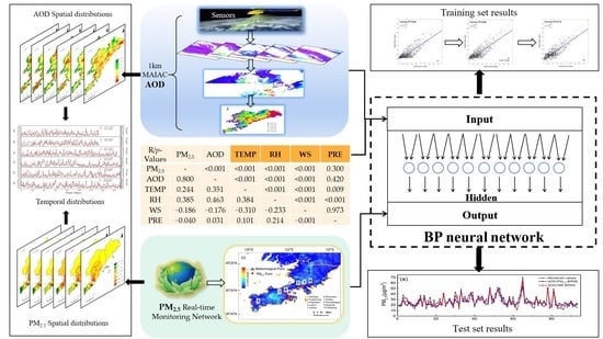
Figure 1. Map of (a) China. Elevation map of (b) Dalian and (c) main urban areas of Dalian. (b) Dalian main urban region and urban–rural region. (c) Spatial distributions of PM2.5 point in Dalian.
Remotesensing 14 01617 g001
Figure 2. BPNN topology.
Remotesensing 14 01617 g002
Figure 3. Establishment of BPNN.
Remotesensing 14 01617 g003
Figure 4. Ten-fold cross validation to determine the number of hidden layer nodes.
Remotesensing 14 01617 g004
Figure 5. Time series of AOD and PM2.5 from 2015 to 2020.
Remotesensing 14 01617 g005
Figure 6. Temporal spatial distribution of PM2.5 and AOD from 2015 to 2020.
Remotesensing 14 01617 g006aRemotesensing 14 01617 g006b
Figure 7. Population density distribution of Dalian in 2020.
Remotesensing 14 01617 g007
Figure 8. Estimated results of AOD–PM2.5 BPNN training set (af).
Remotesensing 14 01617 g008
Figure 9. Estimated results of AOD + meteorological factors–PM2.5 BPNN of training set (a), (a) AOD + TEMP–PM2.5 BPNN, (b) AOD + RH–PM2.5 BPNN, (c) AOD + PRE–PM2.5 BPNN, (d) AOD + WS–PM2.5 BPNN.
Remotesensing 14 01617 g009
Figure 10. Estimated results of AOD + meteorological factors–PM2.5 BPNN of training set (af).
Remotesensing 14 01617 g010aRemotesensing 14 01617 g010b
Figure 11. (af) Simulation diagram of PM2.5 estimated and monitored values of test set. (a) 2015 as the test set. (b) 2016 as the test set. (c) 2017 as the test set. (d) 2018 as the test set. (e) 2019 as the test set. (f) 2020 as the test set.
Remotesensing 14 01617 g011aRemotesensing 14 01617 g011b
Table 1. Correlation coefficient and p-values between PM2.5 and influencing factors at Dalian.
R/p-ValuesPM2.5AODTEMPRHWSPRE
PM2.5-<0.001<0.001<0.001<0.0010.300
AOD0.800-<0.001<0.001<0.0010.420
TEMP0.2440.351-<0.001<0.0010.009
RH0.3850.4630.384-<0.001<0.001
WS−0.186−0.176−0.310−0.233-0.973
PRE−0.0400.0310.1010.214−0.001-
Table 2. Fusion data descriptive statistics.
VariableMinMaxAvgSD
PM2.5 (μg/m3)10.75076.49326.80810.862
AOD0.0251.7760.2890.249
TEMP (°C)−11.50032.30010.23510.533
RH (%)93.00016.00050.73915.248
WS (m/s)3.0388.6003.0381.269
PRE (mm)0.00022.6000.2911.766
Table 3. Dataset division.
Data SetTraining Set (Year)Test Set (Year)
1a (2016, 2017, 2018, 2019, 2020)2015
2b (2015, 2017, 2018, 2019, 2020)2016
3c (2015, 2016, 2018, 2019, 2020)2017
4d (2015, 2016, 2017, 2019, 2020)2018
5e (2015, 2016, 2017, 2018, 2020)2019
6f (2015, 2016, 2017, 2018, 2019)2020
Table 4. BPNN parameters.
Hidden Layer Activation Function Output Layer Activation Function Training Function Target ErrorNumber of IterationsLearning Rate
tansigpurelintrainlm10−530000.1
Table 5. Cross-validation training results of BPNN.
Hidden Layer Neurons
23456789101112
RMSEa10.646.416.4211.6611.1858.4013.5933.7312.0310.3413.71
RMSEb6.446.456.487.506.766.836.806.967.187.237.97
RMSEc6.486.776.827.3210.078.257.4310.8714.6613.4212.48
RMSEd6.4715.7410.4844.4544.4011.4210.7726.5110.5721.5318.61
RMSEe6.396.376.5010.066.806.466.476.838.088.586.82
RMSEf6.496.956.6761.7152.1536.3938.5253.7132.8632.2618.18
Table 6. Estimate results of BPNN model.
Input VariableTest Set (Year)
201520162017
R2RMSEAccR2RMSEAccR2RMSEAcc
AOD0.6406.6680.7%0.6566.5681.4%0.7236.2782.9%
AOD + TEMP0.6616.4782.0%0.6726.4882.0%0.7316.2383.2%
AOD + RH0.6566.5881.9%0.6616.5081.2%0.7296.2383.1%
AOD + PRE0.6486.6081.8%0.6586.5581.9%0.7196.2583.0%
AOD + WS0.6456.6581.7%0.6586.6281.8%0.7116.2682.9%
AOD + All Features0.6766.4582.2%0.6916.3482.7%0.7526.2383.4%
Input VariableTest Set (Year)
201820192020
R2RMSEAccR2RMSEAccR2RMSEAcc
AOD0.6566.3382.0%0.6406.8179.9%0.6406.3481.9%
AOD + TEMP0.6796.2982.7%0.6716.7480.4%0.6616.2082.6%
AOD + RH0.6726.3182.5%0.6546.7780.1%0.6516.2282.6%
AOD + PRE0.6716.3382.2%0.6436.7880.0%0.6536.3182.3%
AOD + WS0.6676.3382.2%0.6426.8079.9%0.6506.3482.0%
AOD + All Features0.6776.3082.8%0.6866.5482.0%0.6636.3282.4%
Table 7. Comparison of model parameters and results.
ModelModel Parameter Model Expression
Hidden NeuronsCgR2RMSE/μg/m3RMSE SD/μg/m3AccTime
BPNN2--0.7236.350.2682.4%2″00-
SVR-40.060.6726.370.2782.2%13″12-
LR---0.6566.420.2282.0%-PM2.5 = 34.28AOD + 17.00
NLR---0.6726.370.2382.2%-PM2.5 = 14.87 + 47.09AOD − 14.16AOD2 + 3.15AOD3
MLR---0.6896.200.2683.4%-PM2.5 = 0.80AOD + 0.07TEMP + 0.04RH − 0.05WS − 0.06PRE
Meteorological factors–SVR-210.6896.250.2883.3%11″29-
Meteorological factors–BPNN2--0.7576.110.2684.4%2″00-
Publisher’s Note: MDPI stays neutral with regard to jurisdictional claims in published maps and institutional affiliations.

