1. Introduction
As earth observation satellite technologies are developing rapidly [
1], more and more advanced sensors may acquire a large amount of remote sensing images at a fast rate with higher spatial, temporal, and spectral resolution [
2,
3,
4,
5]. This leads to an exponential increase in the size of the acquired images, which enhances the abundance of images greatly as well as bringing many challenges for storing and processing the images efficiently [
6,
7,
8]. On the one hand, important and meaningful scientific discoveries may be concluded from the research on analyzing very large amount of remote sensing images on a global scale and a long time series [
9,
10,
11]. How to mine useful knowledge from the archived images efficiently becomes an intractable task. On the other hand, in practical applications, the processing demands in real-time large-scale image processing are also getting higher [
12], especially in the cases of flood or earthquake disasters, which require processing of large-scale images as soon as possible [
13,
14,
15]. Therefore, how best to process the acquired large-scale images in real-time is becoming more urgent and yet difficult [
16].
To process large-scale images rapidly and efficiently in specific applications, the processing tasks should be carried out over a distributed cluster organized by big data frameworks [
17] rather than in multiple independent single machines. This is because the big data framework can pool together the calculation resources of many single machines, and hence gives us the ability to use the cumulative resources as if they were a single computer [
18]. Hence, besides a group of physical machines, a framework coordinating the tasks across multiple calculation nodes is necessary. The Google Earth Engine (GEE) [
19] may be regarded as one kind of framework, which is designed specifically to process large-scale remote sensing images over the cloud platform [
20,
21]. In GEE, massive images are uniformly organized and processed with predefined norms [
22]. It is convenient for users to use images from archived datasets without downloading or processing them locally [
23]. However, GEE lacks the support of several specific remote sensing datasets, and its official image processing algorithms are limited with respect to object-based image analysis [
24] as it focuses more on pixel-based image processing algorithms [
25]. Hence, an alternative way to processing large-scale images is to adopt the commercial big data frameworks, such as the Hadoop [
26], the Spark [
27], and the Flink [
28], to manage and coordinate the tasks over a distributed cluster. Then, we could develop functions more flexible and feasible customized according to various actual demands over distributed cluster with the help of mature frameworks. Hence, to transplant the abundant sequential algorithms to a distributed environment becomes a practical issue and is a feasible scheme to expand the capability of existing algorithms.
It is still a challenge, however, to transplant sequential algorithms directly to a distributed environment to deal with large-scale images. As the multiple calculation nodes could process the subset of large-scale images simultaneously, the computational complexity is approximately linear between the execution time and image volume under a distributed environment. Therefore, the sequential algorithms integrated into a distributed cluster could indeed improve the execution efficiency and enhance its scalability greatly [
29,
30], and acquire identical or similar results as those implemented in a sequential way. However, the sequential algorithms usually need to be reorganized and rebuilt to adapt to a new distributed implementation environment. In addition, incomplete objects usually exist in border areas of image tiles when object-based image analysis methods are implemented in parallel among multiple calculation nodes. The decomposition of large-scale images usually breaks up the objects located on border areas into several parts, which generates incomplete objects with some artifacts [
31]. Moreover, these incomplete objects may lead to inaccurate propagations, which affect the subsequent applications and may limit the scalability. Hence, how best to solve the incomplete object problem efficiency is the key point for transplanting sequential algorithms to a distributed environment.
To solve the incomplete object problem, researchers have developed many related models based on redundant computing to modify incomplete objects during large-scale image processing. The scalable tile-based approach is exploited to process large-scale images and modify incomplete objects, hence Michel, Youssefi [
32] and Lassalle, Inglada [
33] separately presented the mean-shift and the region-merging methods based on the segmented images approach. Furthermore, Derksen, Inglada [
34] proposed the simple linear iterative clustering segmentation (SLIC) algorithms according to the tile-based approach to organize pixels into superpixels in parallel. The parallel segmentation methods were built according to the marginally stable concepts to generate identical or similar results to the sequential ones. However, the marginally stable concept is not suitable for all segmentation algorithms, and the degrees of parallelism are not high enough for the parallel SLIC. Besides the former models, both Lin and Li [
35] and Gu, Han [
36] developed the parallel segmentation algorithms based on the minimum spanning tree model and the minimum heterogeneity rule partitioning technique to modify incomplete objects, but the message passing interface parallel technology is rather complicated for many researchers, as the users concentrate on not only the target algorithm itself but also the task schedules among the calculation nodes. In an attempt to focus more effort on algorithm modifications, Happ, da Costa [
37] proposed a Hadoop-based distributed strategy for a region-growing algorithm to modify incomplete objects with the specific indexing mechanism and hierarchical stitching method, but its adopted MapReduce programming model is relatively slow. To accelerate the calculations, Wang, Chen [
38] proposed a distributed image segmentation model to remove artifacts and modify incomplete objects by repeat calculations based on the faster Apache Spark model; however, the execution time was not recorded and the communication volume of Apache Spark was not optimized well. In order to deal with the aforementioned issues, Chen, Wang [
39] improved the distributed segmentation model in terms of communication reduction by decreasing the auxiliary bands and detecting the buffer sizes automatically. However, the extra auxiliary bands not only waste the calculation memory but also generate large communications during the shuffle stage, and also limit the efficient processing of the distributed strategy. In addition, most of the described strategies modify incomplete objects by redundant computing. Hence, it is necessary to remove the extra auxiliary bands, optimize the volume during the shuffle stage, and reduce the redundant computing to improve the efficiency a lot further.
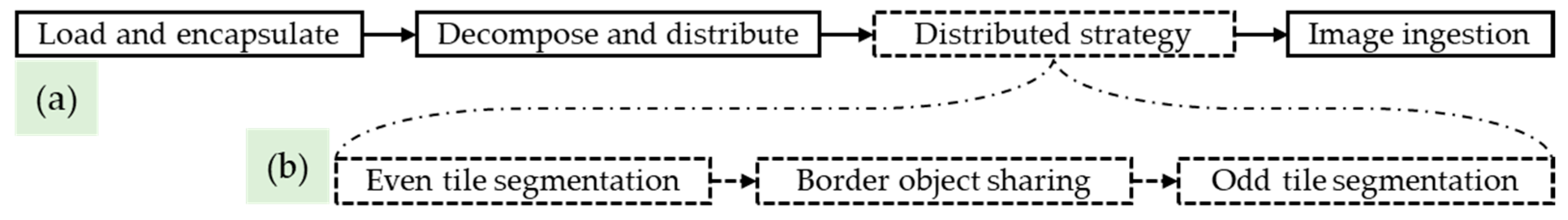
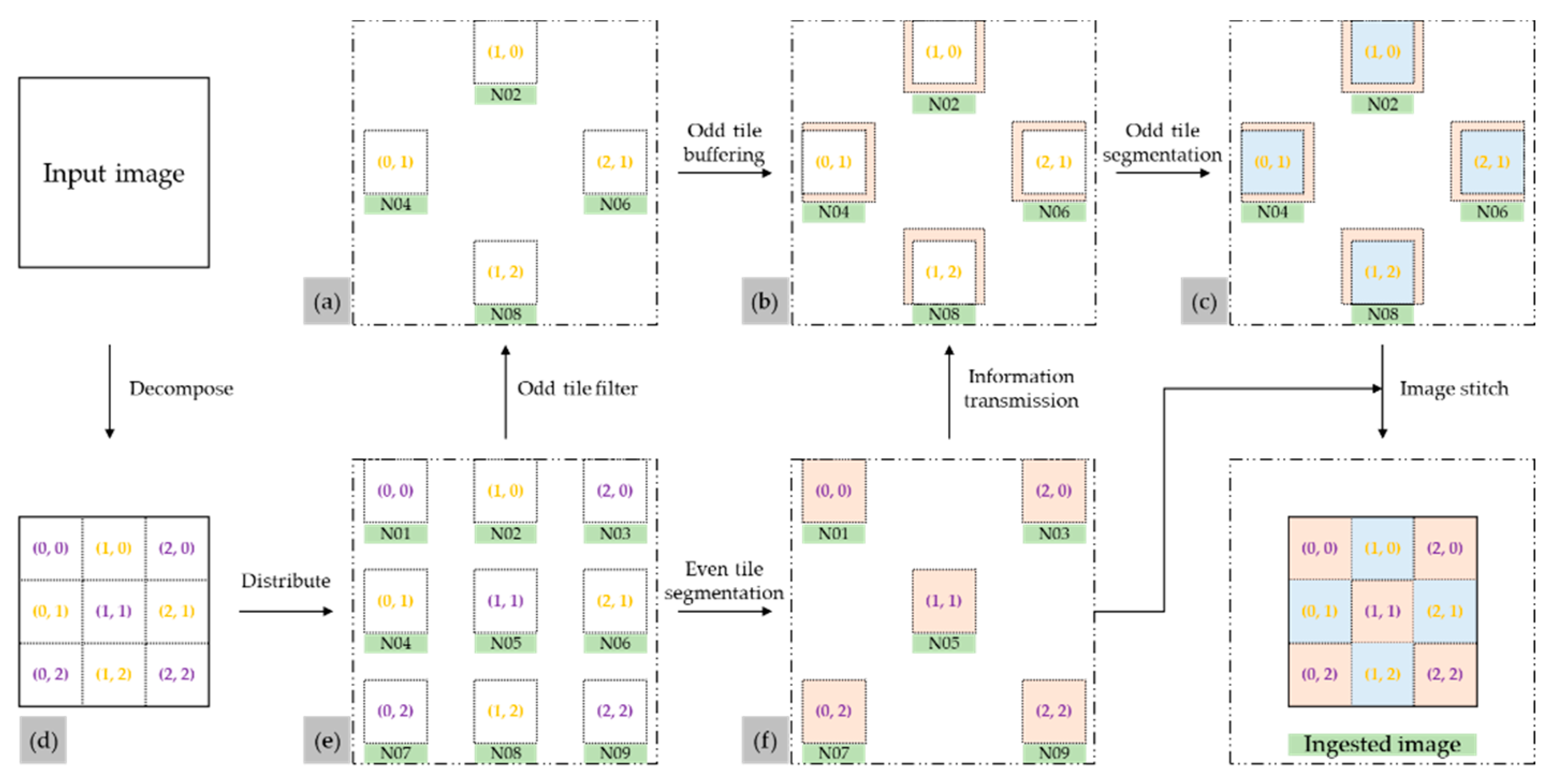
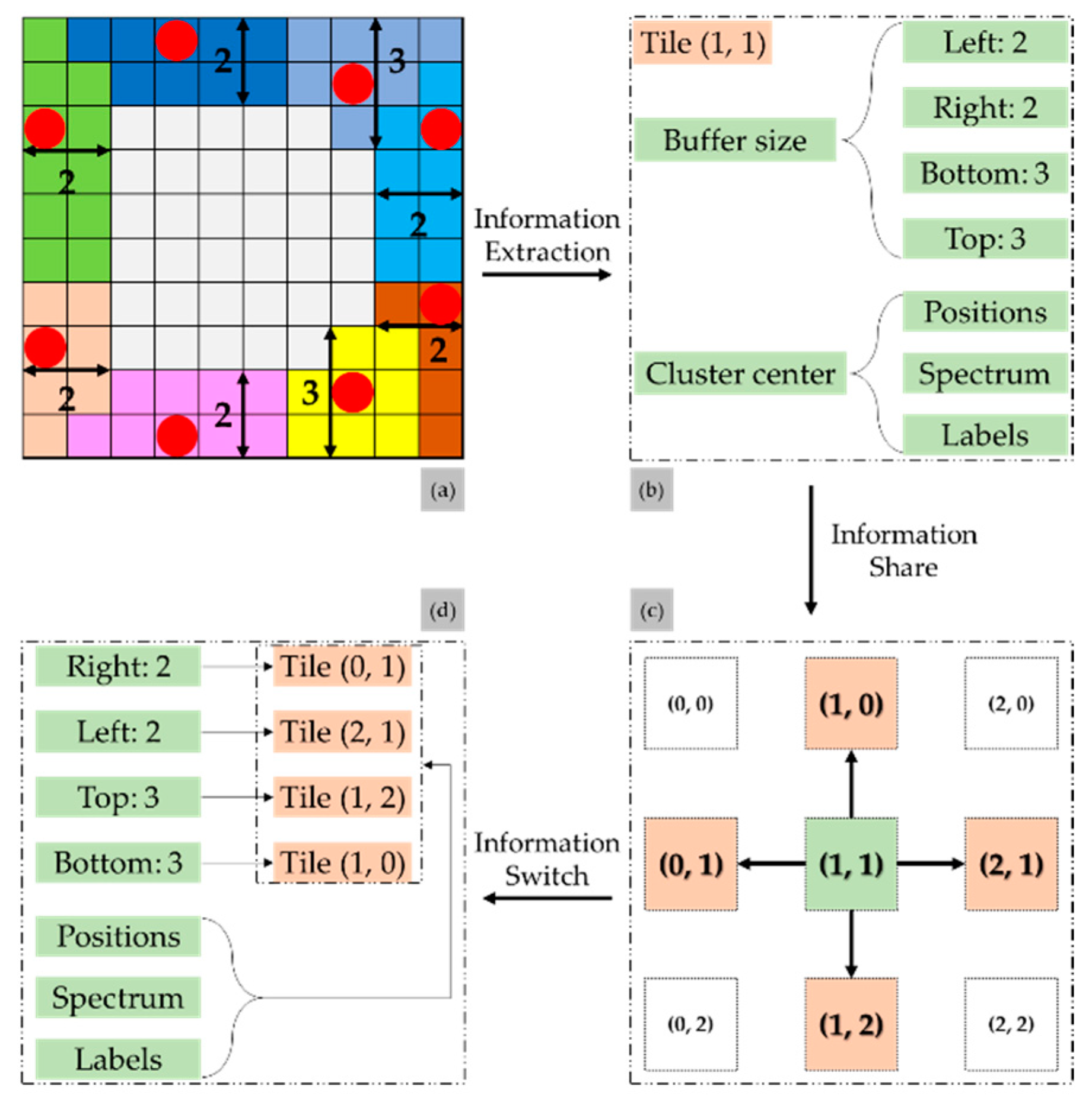
In this study, to further improve the efficiency of previous strategies, a new distributed strategy based on Apache Spark is proposed to solve the incomplete object issues of integrating sequential SLIC algorithms into a distributed cluster. The massive image tiles, generated by loading, decomposing, and distributing operations on a large-scale image, were divided into two categories—the even tiles and the odd tiles—according to their index. First, the even tiles were segmented independently and simultaneously by the SLIC algorithm. Then, the cluster centers and buffer sizes of four aspects (the left, the right, the bottom, and the top aspects of image tiles) of even tiles were acquired and encapsulated into the accumulator structure without employing extra auxiliary bands to record immediate results. The buffer sizes and cluster centers in the accumulator were switched from even tiles to odd tiles, and broadcasted around the distributed cluster. During the shuffle stage, the odd tiles acquired pixels from surrounding even tiles according to the buffer size for each aspect. The SLIC algorithm was used to segment the enlarged odd tiles again with the support of buffered pixels and cluster centers. Specifically, all pixels of the large-scale image were segmented only once without redundant computing to modify the incomplete objects. After the segmentation, the final segmentation results were generated by the ingestion operation. The proposed strategy was then evaluated in terms of the accuracy and execution efficiency to reveal its performance.
The main objectives of the research were to:
Modify incomplete objects by remaining to enlarge the superpixels, generated in even tiles, with shared cluster centers in odd tiles;
Employ the shared variables of Apache Spark to record intermediate results rather than introducing extra auxiliary bands;
Improve the efficiency by implementing shuffle operations among approximately half of the entire image tiles.
The organization of this paper is as follows.
Section 2 describes the methods.
Section 3 outlines the experimental design.
Section 4 presents the results, and this is followed by the discussion in
Section 5. Concluding remarks are given in the last section.
5. Discussion
From the perspective of
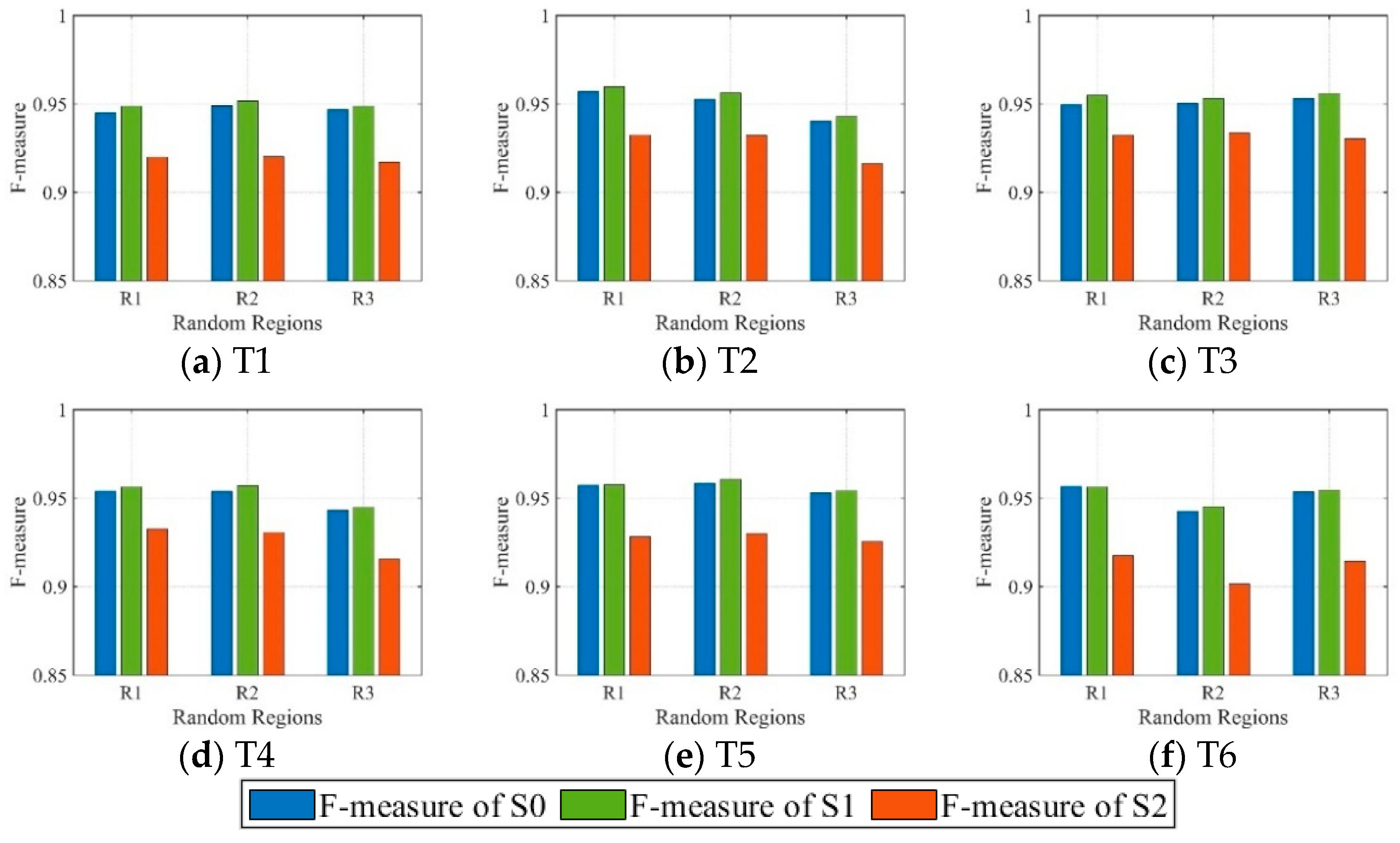
Figure 5 and
Figure 6, the F-measure values of S0 and S1 were very similar with each other in all random regions. Furthermore, the F-measure values of S2 were not only less than S0 but also less than S1 in all cases. As known to us, the strategy of S2 has been proposed and its efficiency proved with F-measure metrics in several experiments, where it also achieves better performance than corresponding comparison strategies in these cases [
38,
39]. This situation may be caused by the characteristics of the testing segmentation algorithm. The SLIC algorithm is a classical superpixel generation method which could produce the square-like superpixels with defined size and regular shape. In general, the actual landscape object is usually split by the superpixel boundary into two or more parts if it is far bigger than the superpixel size. Therefore, the edge of image tiles is often the boundary for many superpixels. The inner superpixels of S0, S1, and S2 in identical locations were approximately the same as each other, so the minimum F-measure of comparison strategies in random regions was relatively high. Hence, the border area processing of our strategy is more suitable for the characteristics of the SLIC algorithm compared with S2, which follows the repeating calculation rules.
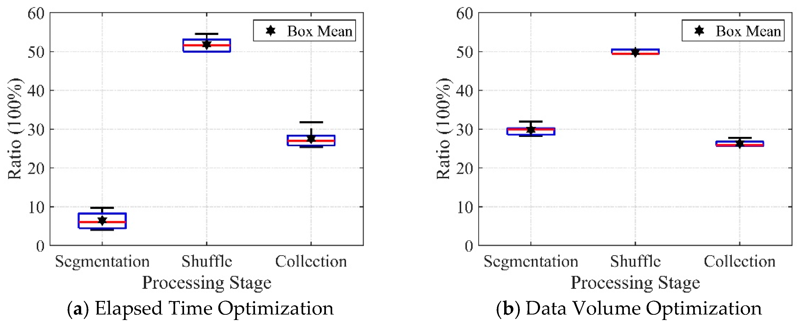
In efficiency evaluation experiments, the acquired 10 repeated execution time is usually different although implemented with identical parameters, and this situation always appeared in our experiment. Although this is mainly caused by the hardware conditions of distributed cluster and the task scheduling circumstances of Apache Spark, the general trend for each case could be discerned by recording redundancy data. Moreover,
Figure 7 and
Figure 8 with scatter points could also reflect the actual trend of the experiment. In terms of the execution time, both S1 and S2 took a far longer time than S0. The strategy of S2 needs the repeat calculations to modify the incomplete superpixels, which consumes some time. The strategy of S1 removes the repetition calculation characteristics of S2 and modifies incomplete superpixels of image tiles by enlarging the superpixels with shared cluster centers. However, the even and odd tiles of S1 must be processed in two different times, and the odd tiles could not be processed until the even tiles finished the processing task completely. In contrast, the strategy of S0 just segments image tiles without any border area operations, so it is significantly faster than the other two strategies.
We can see that the execution time of experiment with eight executors is faster than that with four executors, and the difference between S1 and S2 is larger in the latter case under identical parameters. On the one hand, the number of executors could weaken the advances of S1 with respect to S2, as the map operation is seeming like an average of the total execution time in a sequential way. Hence, the higher the number of executors, the less the execution time difference between the two strategies. On the other hand, the adopted large-scale images are not large enough, and the larger the image size, the more advances the strategy would present. In addition, the partition method of Apache Spark could also influence the execution time, as the default partition method was used in all experiments. It may cause the waiting problem among calculation nodes, which leads to S1 just bringing less advances in most cases.
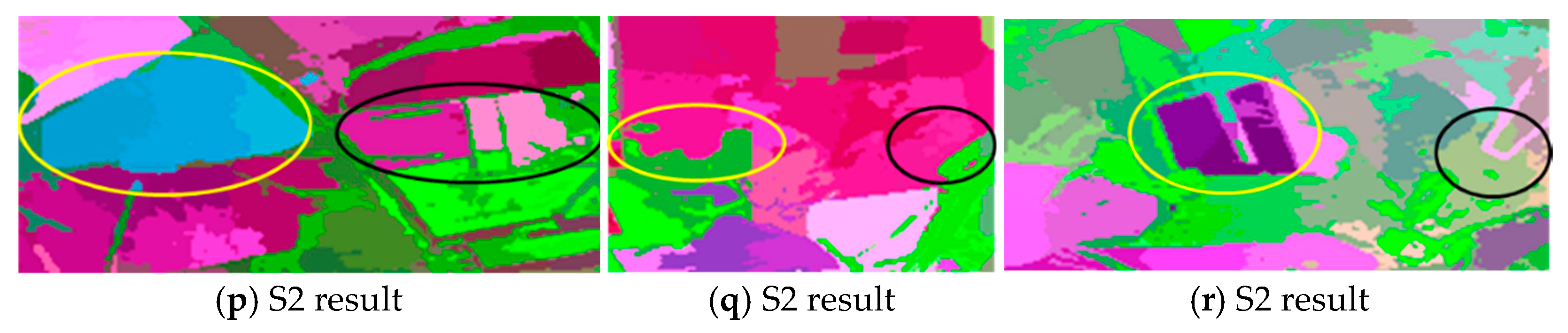
As can be seen the results visually in
Figure 13, the superpixels generated by S1 in the black circle of
Figure 13n were different from that of
Figure 13h. This situation is mainly caused by the characteristics of our strategy, as the even tiles were segmented firstly, whose superpixels remained fixed till the end. In addition, our research did not evaluate the segmentation results with unsupervised models, because all the segmentation operations are strictly based on the theory of SLIC algorithm in entire calculations. Hence, the superpixels generated by each strategy are credible in terms of the unsupervised metrics.
6. Conclusions
In the satellite earth observation field, there is an ongoing exponential increase of the data volume, which brings new challenges for conventional image processing. To this end, employment of sequential algorithms to process large-scale images over the distributed cluster is becoming a new research field. However, most sequential algorithms directly transplanted to the distributed environment would cause incomplete object issues in border areas of the image tiles. To implement sequential algorithms over the distributed cluster conveniently, the SLIC algorithm was selected as the study example to address the incomplete object issue. To this end, a new distributed image segmentation strategy based on the big data platform—Apache Spark—was proposed. A large-scale image was loaded and decomposed into multiple image tiles. All the image tiles were divided into even and odd tiles, which participated in two independent calculation processes, according to the indexes. First, the even tiles were split into superpixels by the SLIC algorithm. Second, the locations of the cluster centers and the buffer sizes of each aspect of even tiles were recorded, extracted, and managed by the shared variables, which were analyzed and organized as prior information. Then, the odd tiles were shuffled to acquire the pixels of the even tiles based on the buffer sizes. Meanwhile, the buffered odd tiles were segmented by the SLIC algorithm using the same parameters as the even tile segmentation with the help of the prior information. Finally, the even and odd tiles were ingested from the calculation nodes to the master node to acquire final result. According to the performance evaluation results, the proposed strategy resulted in improved F-measure values and faster run times than the comparison strategies. In addition, the increases in the execution efficiency trends along with the decreasing executor numbers mean the proposed strategy could run faster with limited calculation resources. The new strategy modifies the incomplete superpixels well by enlarging the superpixels with shared cluster centers and optimizes the communications by carrying out the shuffle operations among only approximately half of entire image tiles. These changes not only improved the accuracy but also increased the execution efficiency and reduced the data volume transmission over Apache Spark. Hence, the proposed strategy is more suitable for the superpixel algorithms as its superpixels are more similar to those in the reference images.
In future work, the new distributed strategy should be tested in larger-scale images. Some optimized operations should also give focus to the partition method of Apache Spark to remove cases of data skew and improve execution efficiencies. In addition, further applications should address practical demands rather than just stand on image segmentation.


