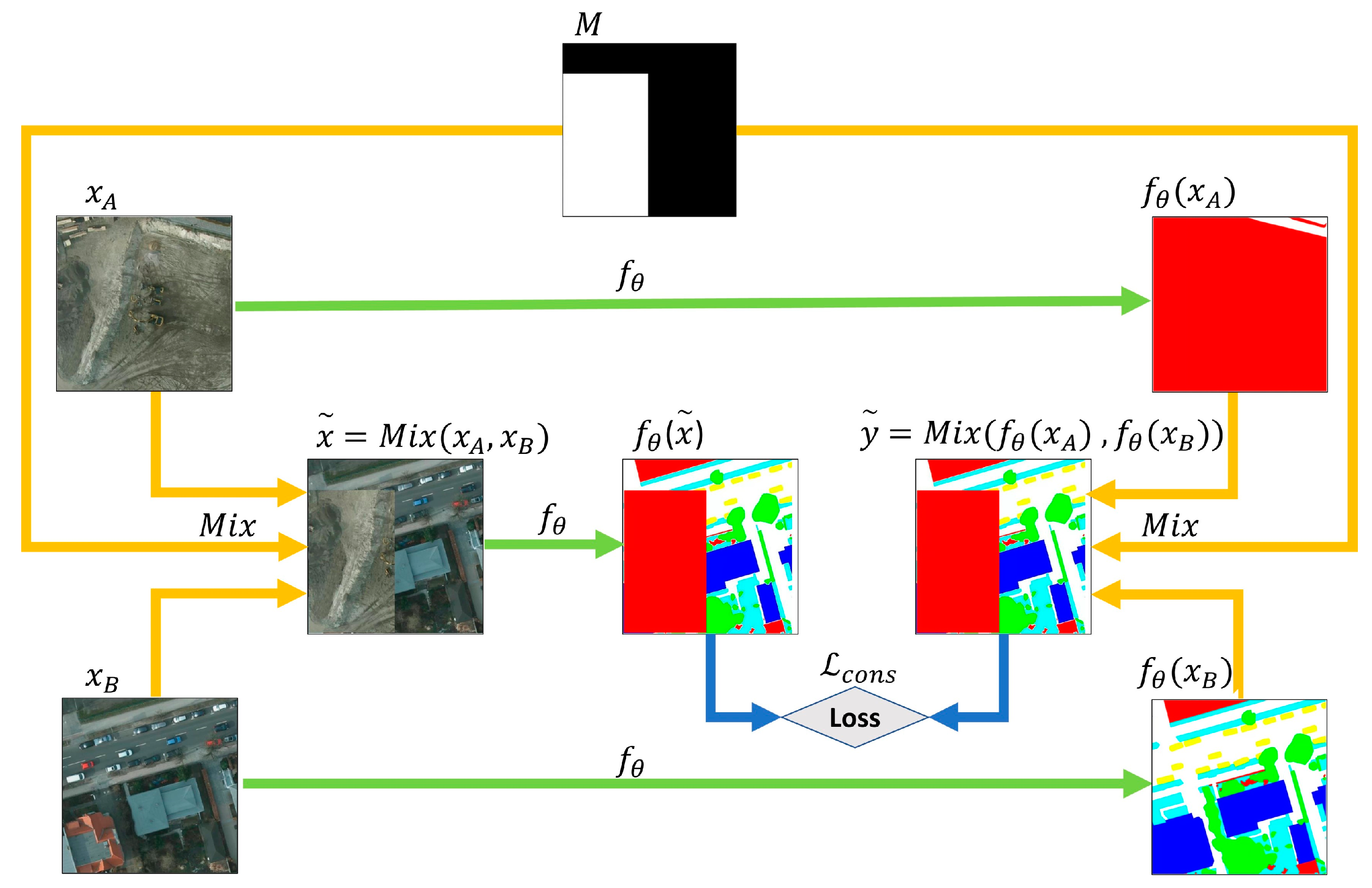
Figure 1.
Illustration of CutMix for SSL semantic segmentation: and are two unlabeled images, and is a DL model for semantic segmentation. We input and to the model and obtain the respective predictions and , then mix them based on a mask and achieve a mixed prediction . At the same time, we mix and into based on the same mask , and feed it to the model to get the predictions ). Finally, the consistency loss can be calculated in terms of the differences between ) and .
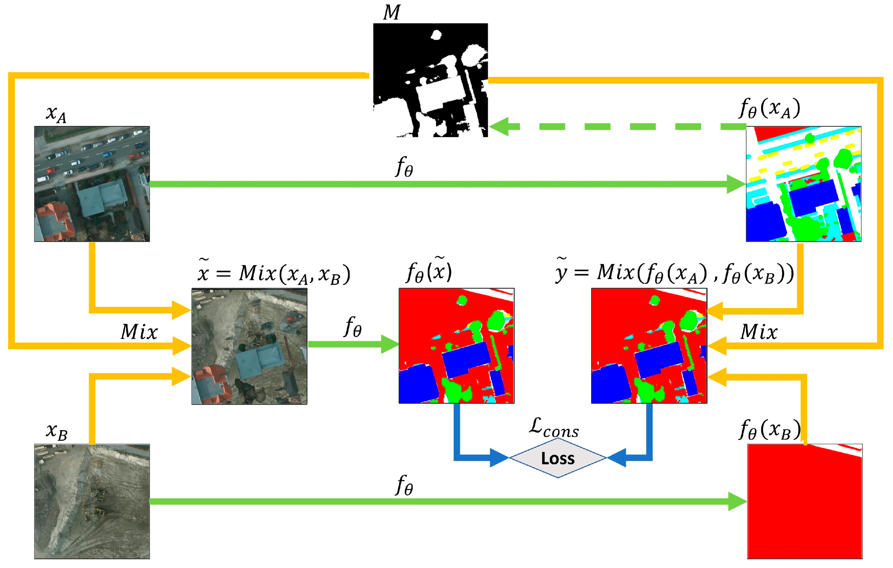
Figure 2.
Illustration of ClassMix for SSL semantic segmentation. The only difference from CutMix is that the mask is generated by the prediction of instead of a random combination of rectangular areas.
Figure 2.
Illustration of ClassMix for SSL semantic segmentation. The only difference from CutMix is that the mask is generated by the prediction of instead of a random combination of rectangular areas.
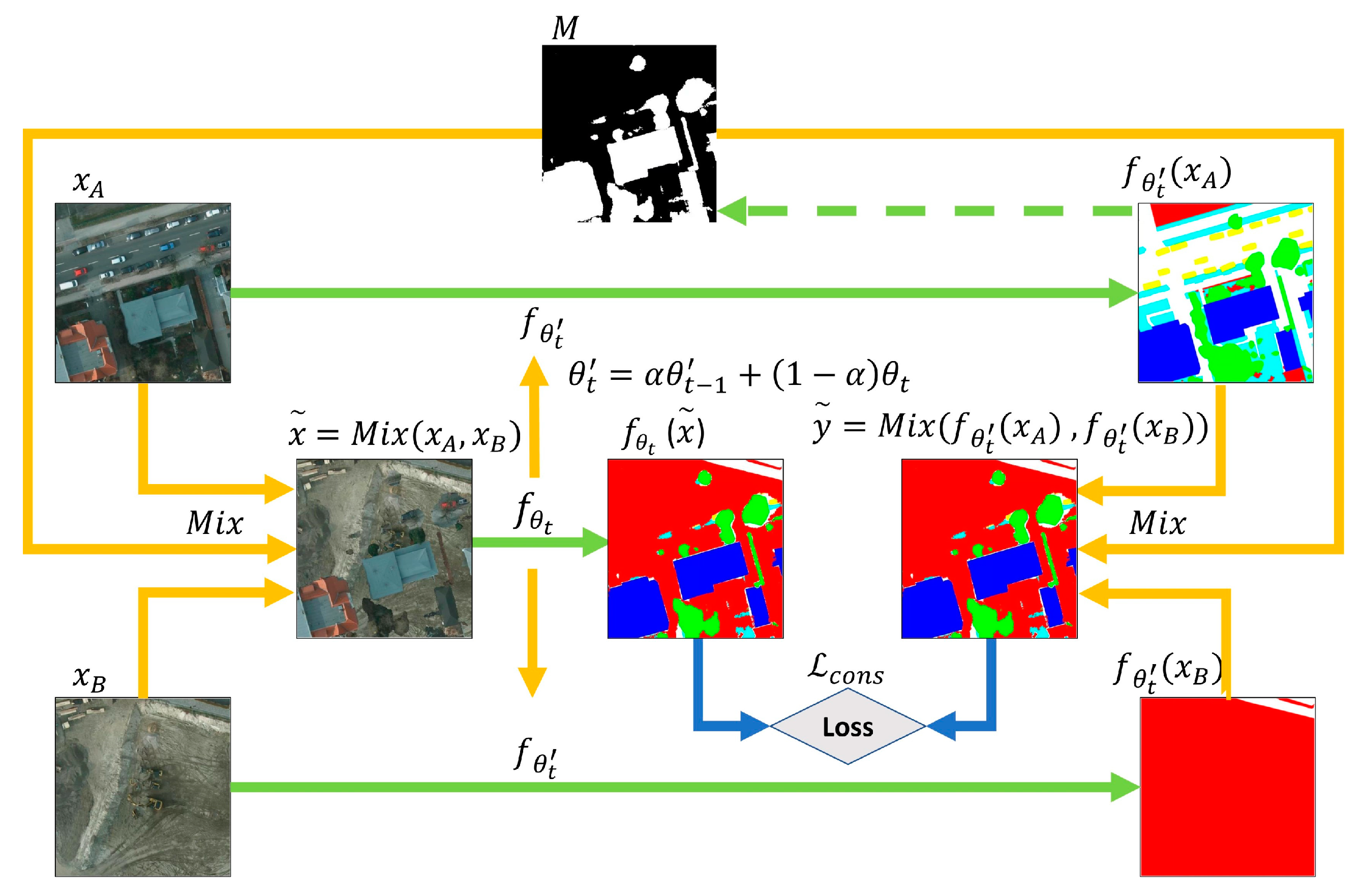
Figure 3.
Illustration of MT for SSL semantic segmentation: There is a student model and a teacher model in training. The student model is the main model trained with the training data. As the training goes on, the teacher model is updated with an exponential moving average of the student model’s parameters, so that a consistency loss can be established based on the respective predictions from the teacher and student models. Note that the parameters of the teacher model do not take part in the process of error backpropagation, and the symbol “//” signifies the stop-gradient.
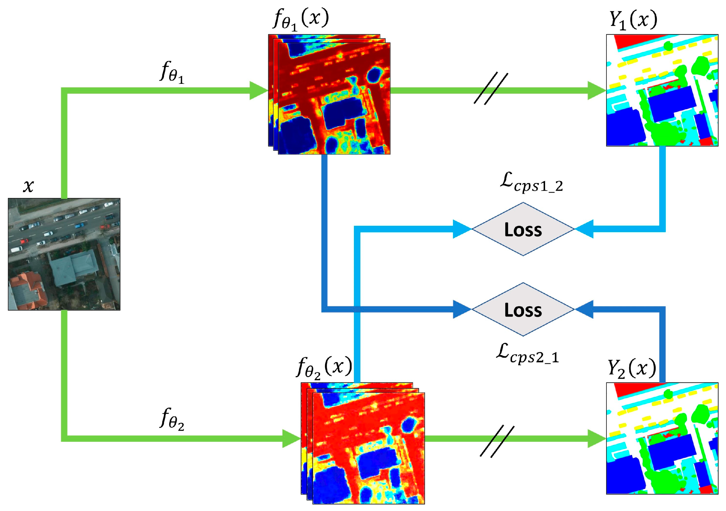
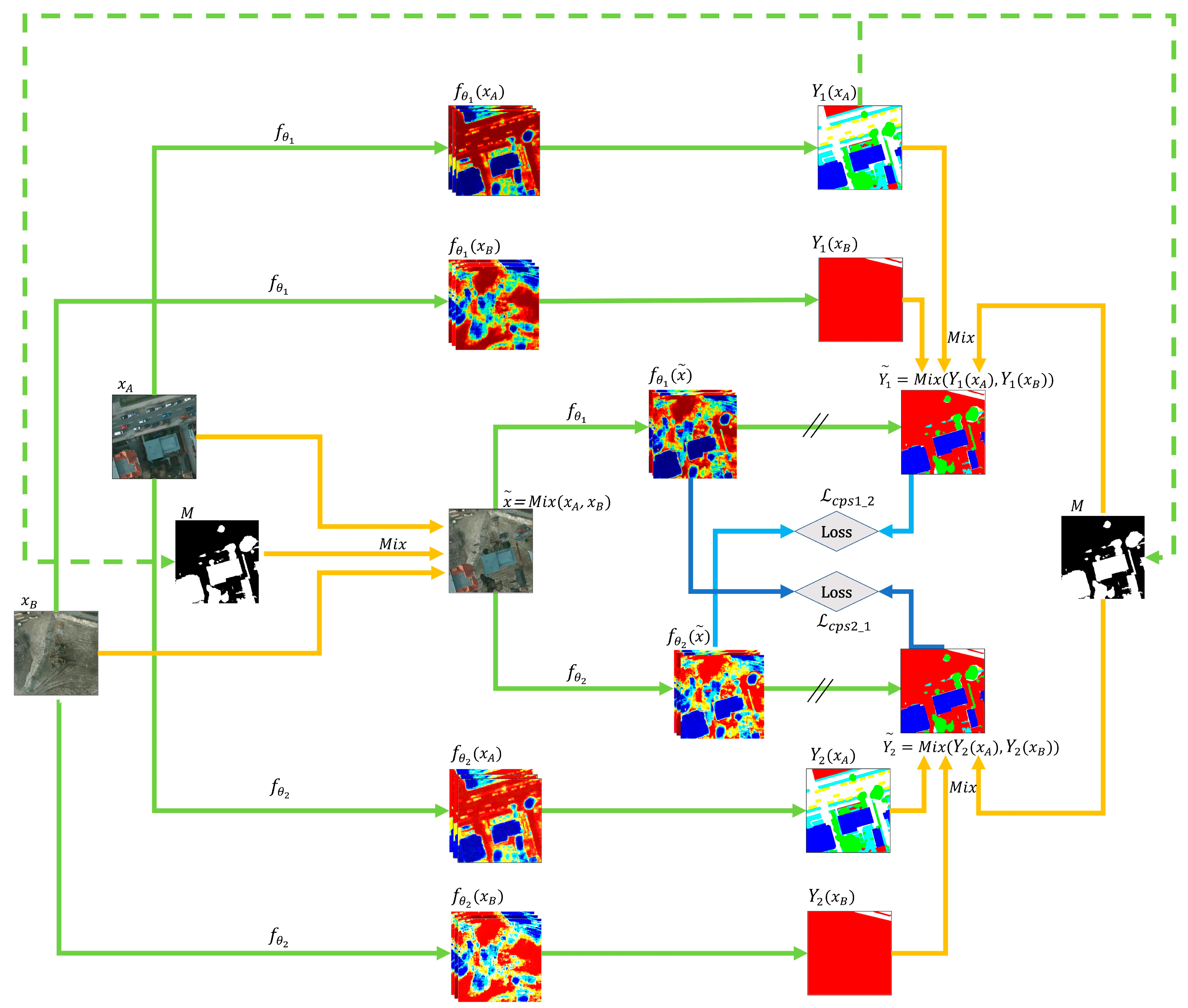
Figure 4.
Illustration of CPS for SSL semantic segmentation: We input image x into the model and , then get the corresponding probability maps and and pseudo-labels and . Subsequently, let supervise and supervise , constructing two consistency losses and , respectively. The symbol “//” signifies the stop-gradient.
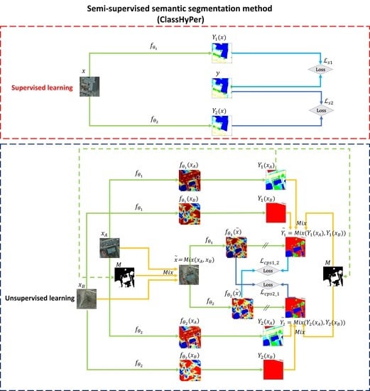
Figure 5.
Illustration of the ClassHyPer approach for SSL semantic segmentation.
Figure 5.
Illustration of the ClassHyPer approach for SSL semantic segmentation.
Figure 6.
Illustration of the hybrid of MT and ClassMix for SSL semantic segmentation.
Figure 6.
Illustration of the hybrid of MT and ClassMix for SSL semantic segmentation.
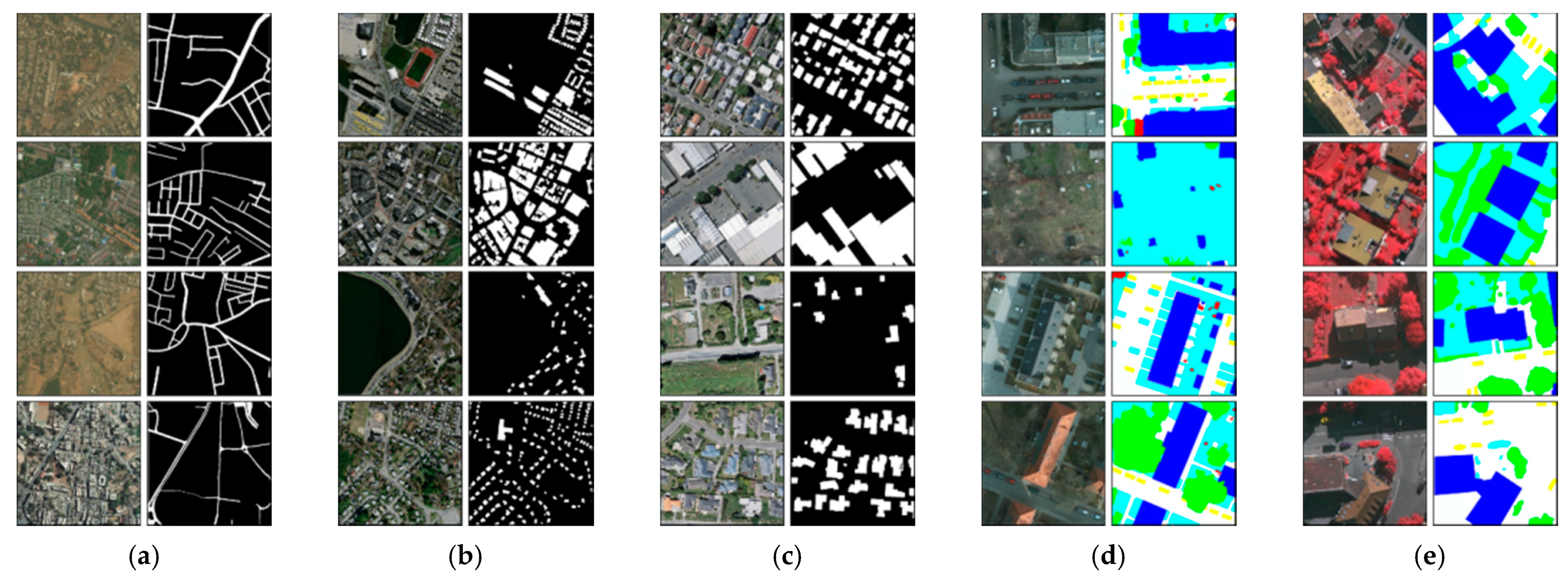
Figure 7.
Examples of the (a) DG_Road, (b) Massa_Building, (c) WHU_Building, (d) Potsdam, and (e) Vaihingen datasets. The left and right columns of each dataset denote the images and corresponding ground-truth labels, respectively.
Figure 7.
Examples of the (a) DG_Road, (b) Massa_Building, (c) WHU_Building, (d) Potsdam, and (e) Vaihingen datasets. The left and right columns of each dataset denote the images and corresponding ground-truth labels, respectively.
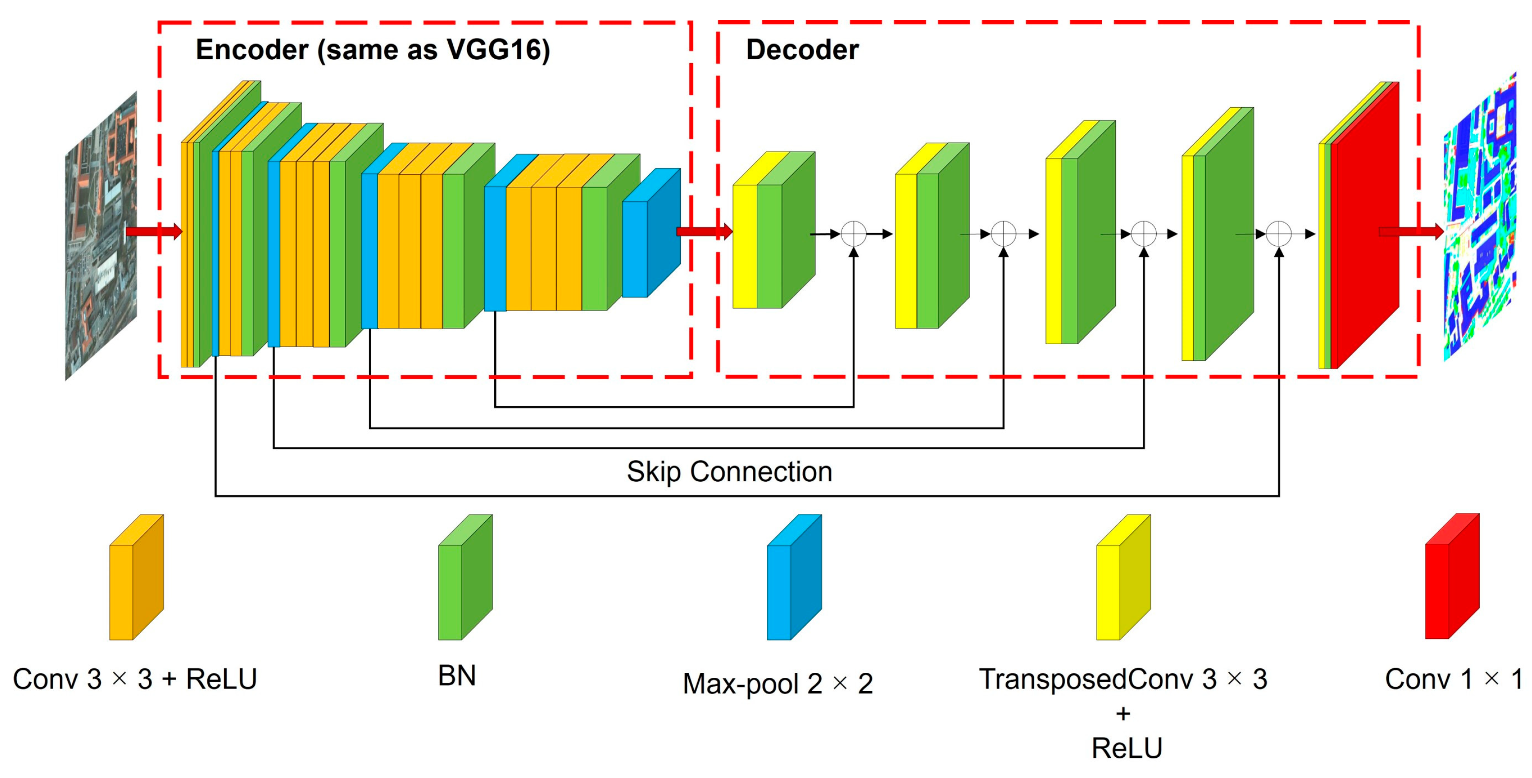
Figure 8.
The architecture of the modified FCN model.
Figure 8.
The architecture of the modified FCN model.
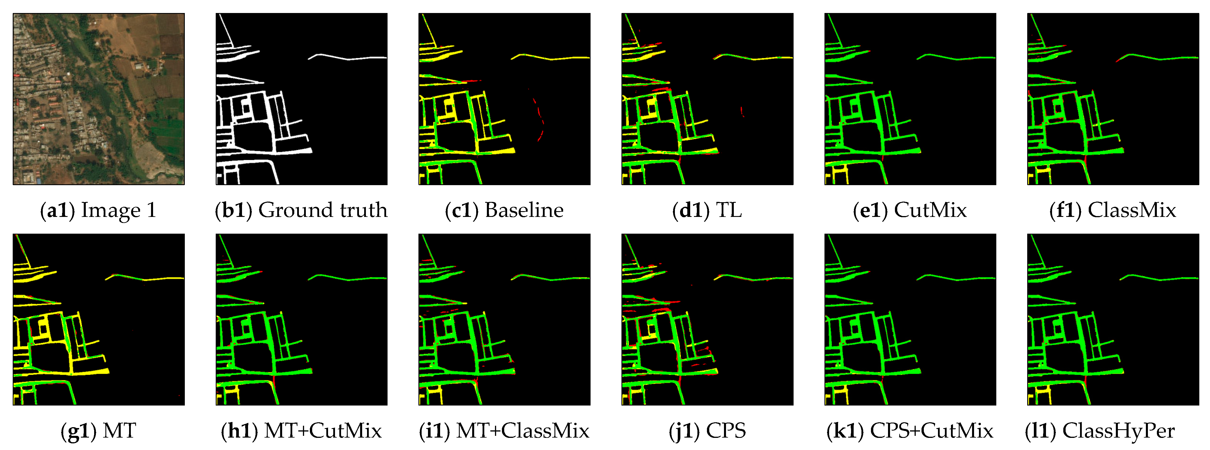
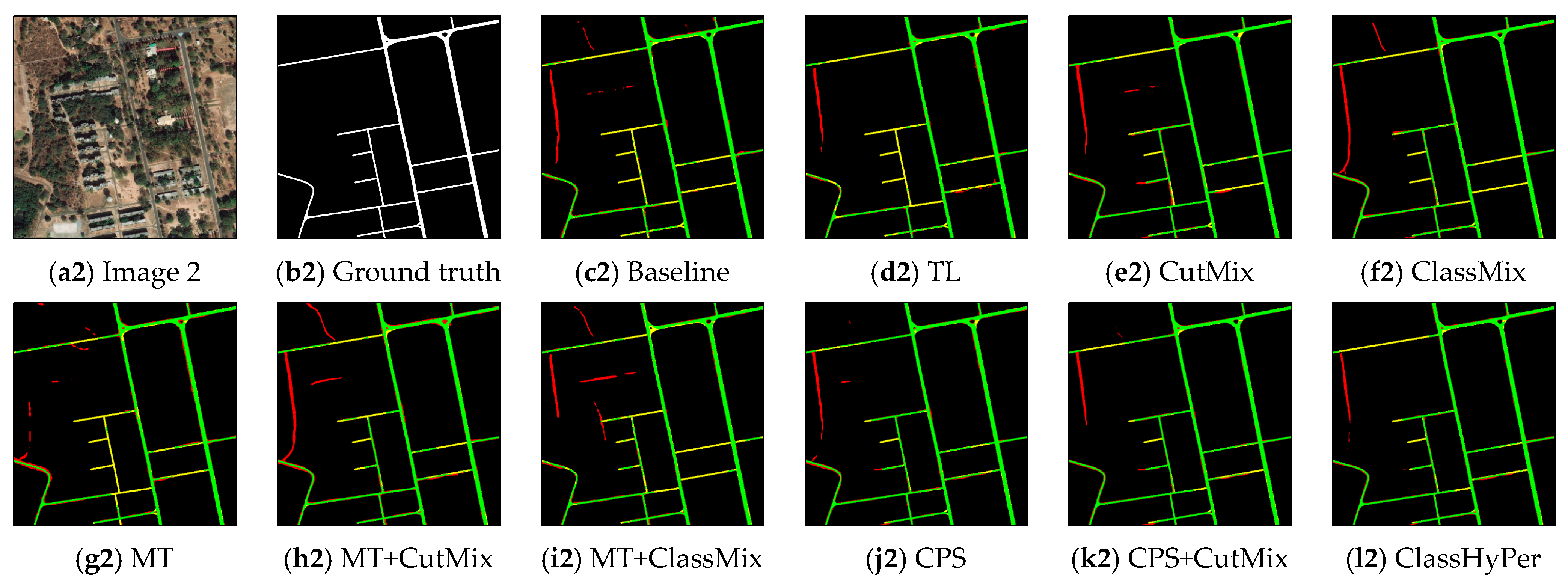
Figure 9.
Visualization results of semantic segmentation using 5% labels from the DG_Road dataset. From (c) to (l), green, yellow, and red color true positive, false negative, and false positive pixels, respectively.
Figure 9.
Visualization results of semantic segmentation using 5% labels from the DG_Road dataset. From (c) to (l), green, yellow, and red color true positive, false negative, and false positive pixels, respectively.
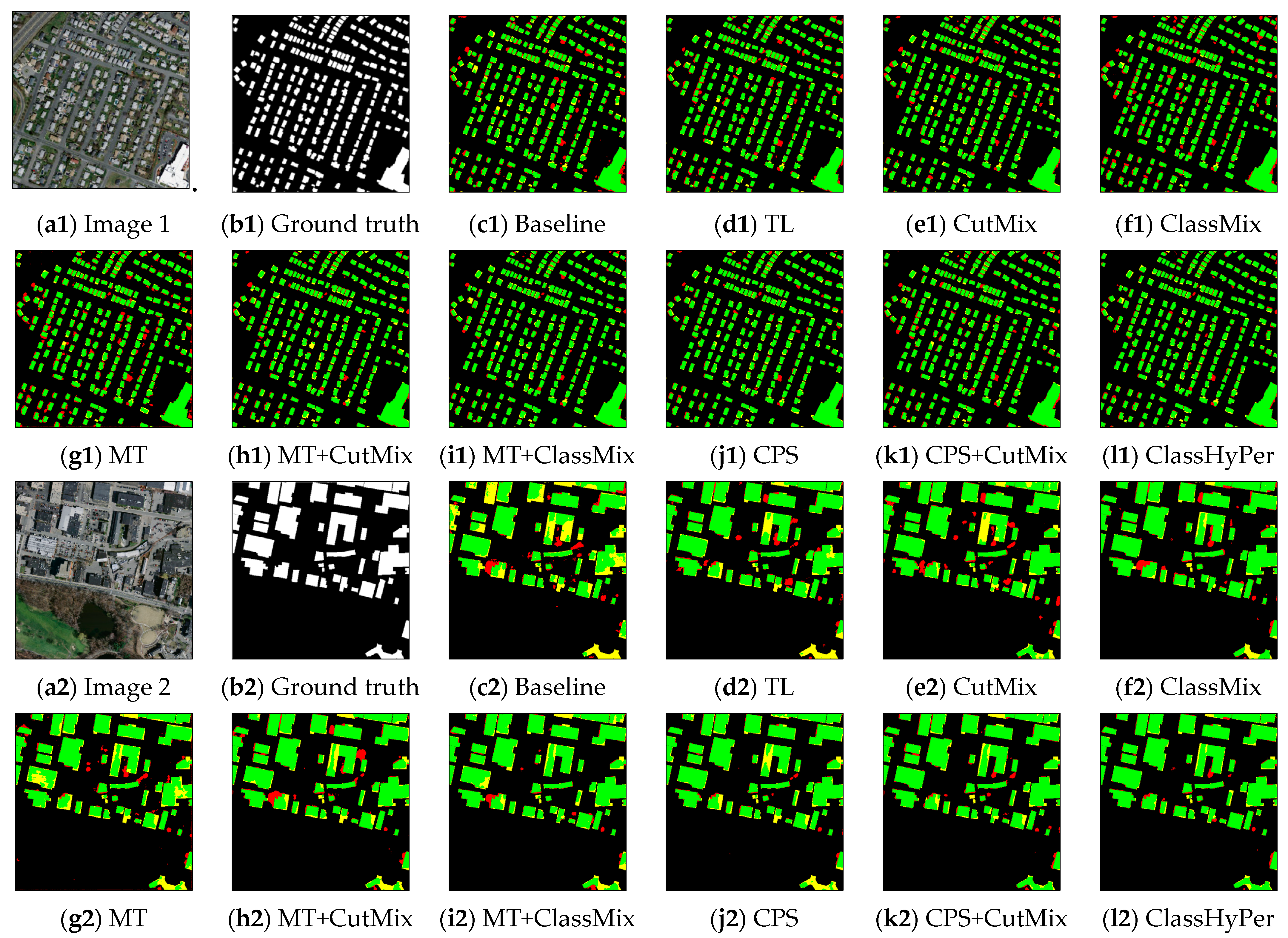
Figure 10.
Visualization results of semantic segmentation using 5% labels from the Massa_Building dataset. From (c) to (l), green, yellow, and red represent true positive, false negative, and false positive pixels, respectively.
Figure 10.
Visualization results of semantic segmentation using 5% labels from the Massa_Building dataset. From (c) to (l), green, yellow, and red represent true positive, false negative, and false positive pixels, respectively.
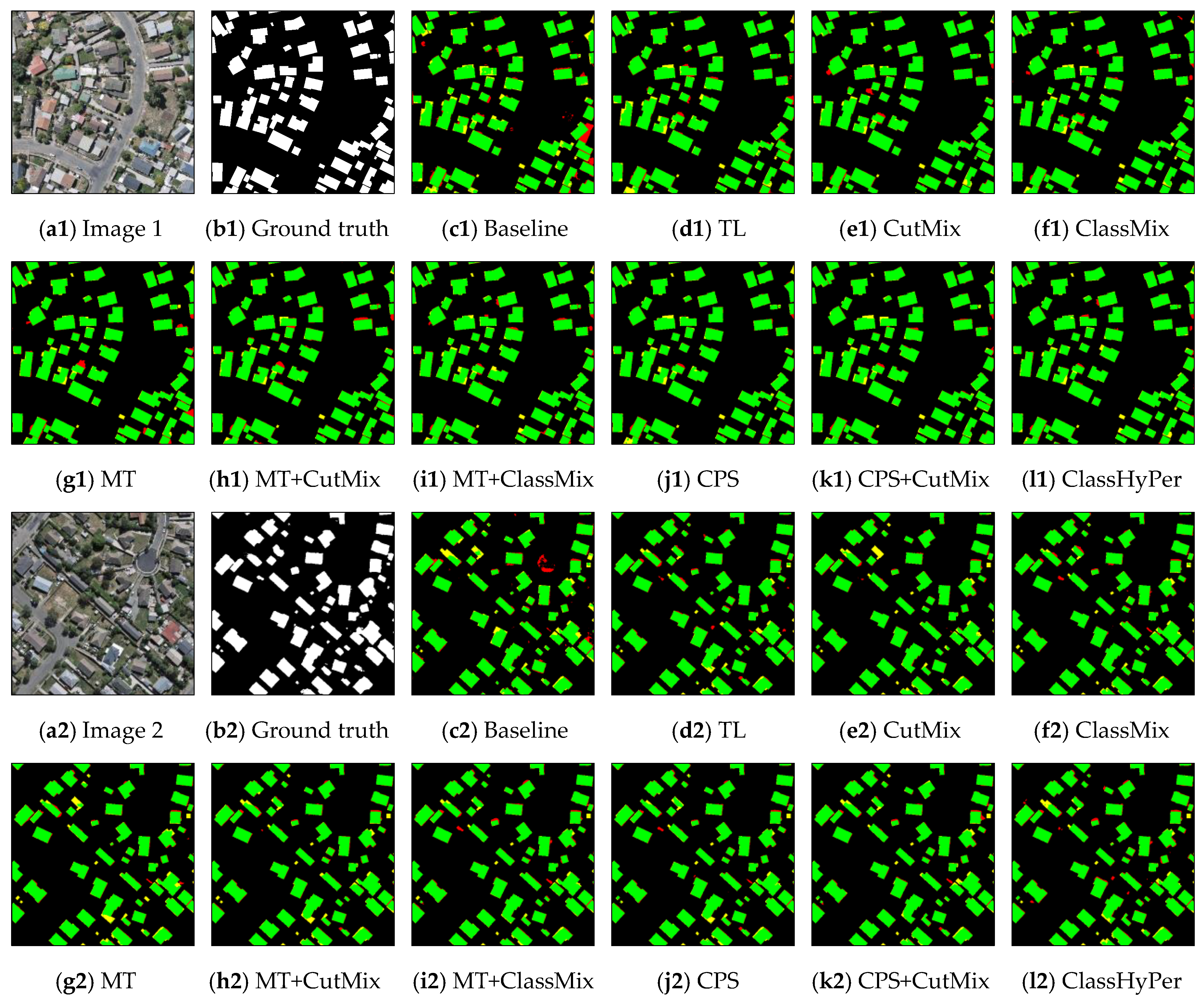
Figure 11.
Visualization results of semantic segmentation using 5% labels from the WHU_Building dataset. From (c) to (l), green, yellow, and red represent true positive, false negative, and false positive pixels, respectively.
Figure 11.
Visualization results of semantic segmentation using 5% labels from the WHU_Building dataset. From (c) to (l), green, yellow, and red represent true positive, false negative, and false positive pixels, respectively.
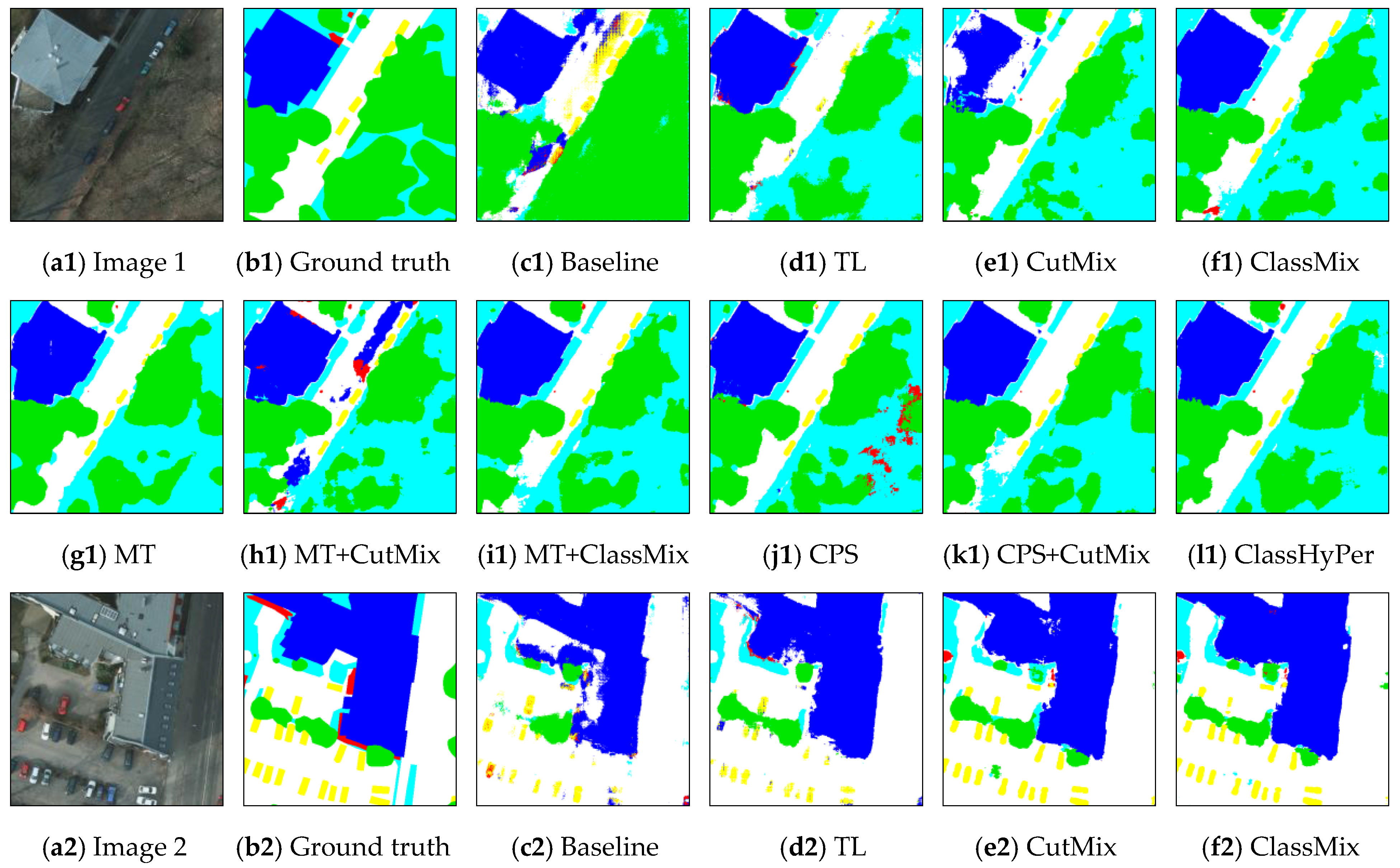
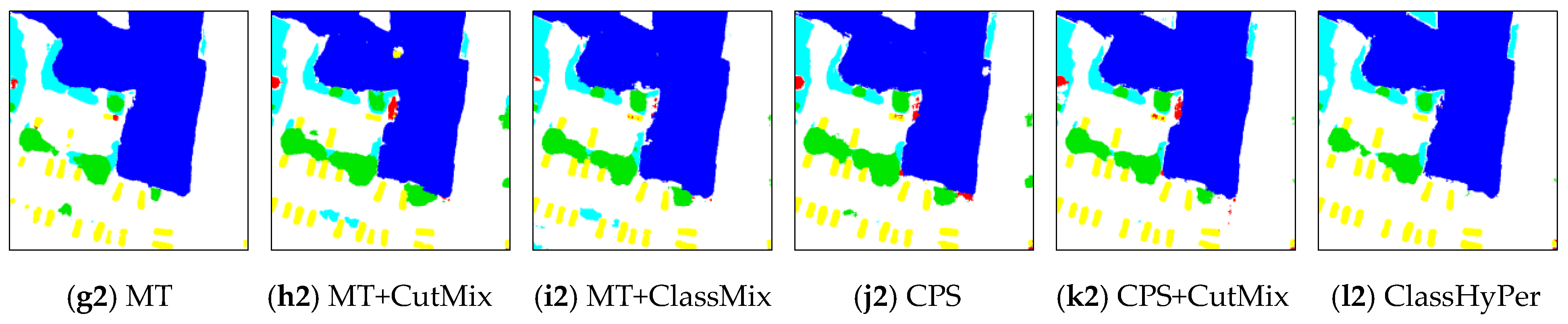
Figure 12.
Visualization results of semantic segmentation using 5% labels from the Potsdam dataset. From (c) to (l), the different colors represent the pixels with different categories, i.e., white (impervious surfaces), blue (building), cyan (low vegetation), green (tree), yellow (car), red (clutter/background).
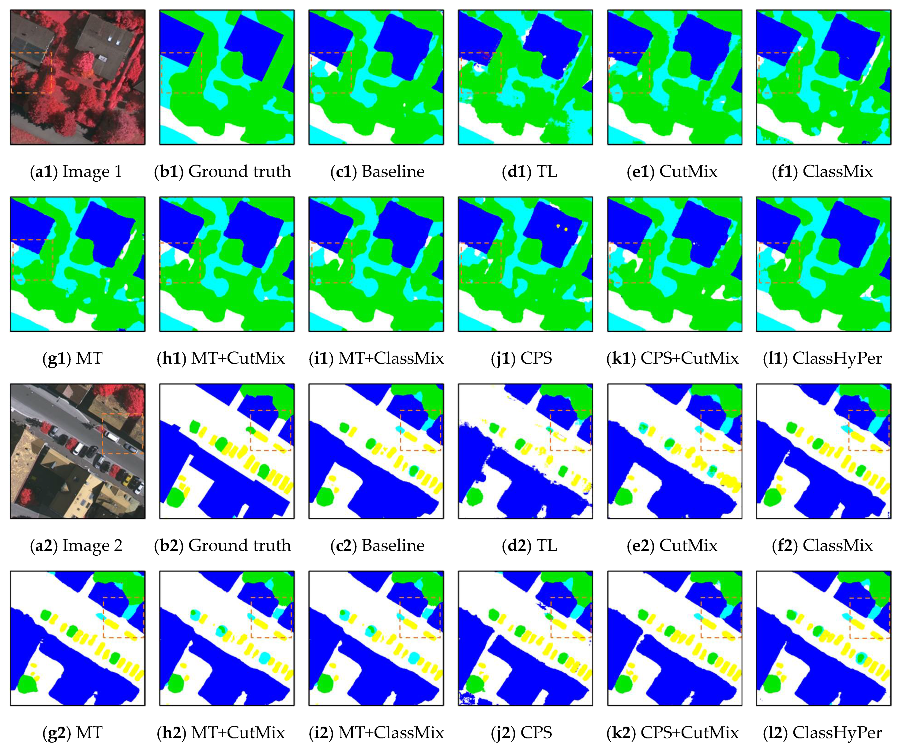
Figure 13.
Visualization results of semantic segmentation using 5% labeled data from the Vaihingen dataset. From (c) to (l), the different colors represent the pixels with different categories, i.e., white (impervious surfaces), blue (building), cyan (low vegetation), green (tree), yellow (car), red (clutter/background).
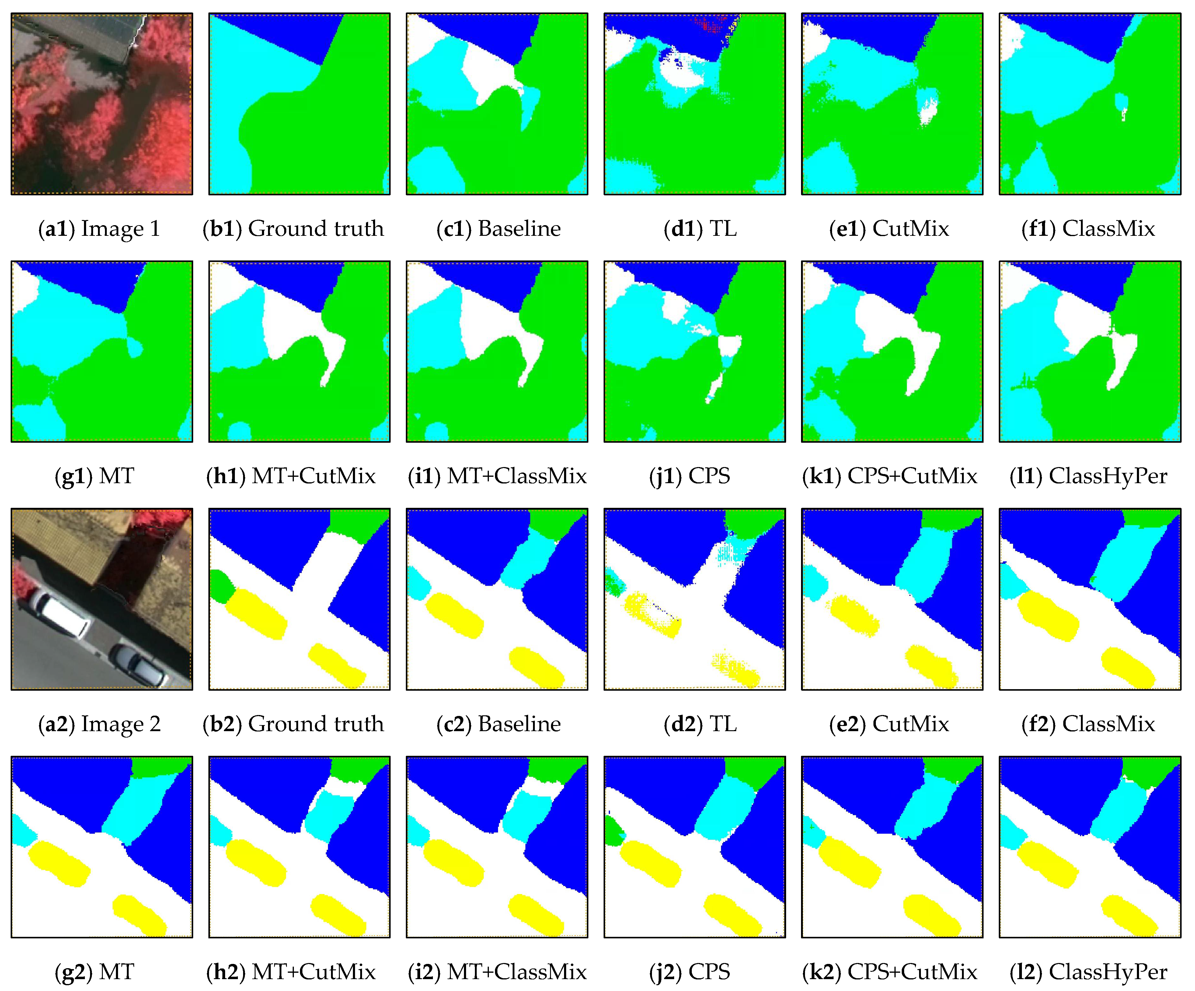
Figure 14.
Enlarged results of the area surrounded by the orange rectangle in
Figure 13. From (
c) to (
l), the different colors represent the pixels with different categories, i.e., white (impervious surfaces), blue (building), cyan (low vegetation), green (tree), yellow (car), red (clutter/background).
Table 1.
Overview of the datasets used in the experiments.
Table 1.
Overview of the datasets used in the experiments.
| Dataset | Labeled
Images | Split (Train:Val:Test) | Classes | Size
(Pixels) | Resolution (m) | Bands | Data Source |
|---|
| DG_Road | 6226 | 3735:623:1868 | 2 | 512 × 512 | 1 | R-G-B | Satellite |
| Massa_Building | 1191 | 1065:36:90 | 2 | 512 × 512 | 1 | R-G-B | Aerial |
| WHU_Building | 8188 | 4736:1036:2416 | 2 | 512 × 512 | 0.3 | R-G-B | Aerial |
| Potsdam | 1368 | 612:252:504 | 6 | 512 × 512 | 0.1 | R-G-B | Aerial |
| Vaihingen | 1009 | 692:68:249 | 6 | 512 × 512 | 0.09 | IR-R-G | Aerial |
Table 2.
Accuracy (, %) comparison of different methods on the DG_Road dataset, where the values in bold are the best for each proportion.
Table 2.
Accuracy (, %) comparison of different methods on the DG_Road dataset, where the values in bold are the best for each proportion.
| Method | 5% (186) | 10% (373) | 20% (747) | 50% (1867) | 100% (3735) |
|---|
| Sup | Baseline | 46.65 ± 0.54 | 50.72 ± 0.83 | 55.80 ± 0.27 | 60.15 ± 0.25 | 62.97 ± 0.07 |
| TL | 52.88 ± 0.39 | 56.76 ± 0.11 | 59.34 ± 0.25 | 62.49 ± 0.21 | 64.73 ± 0.38 |
| SSL | CutMix | 55.63 ± 0.33 | 58.33 ± 0.33 | 60.62 ± 0.11 | 62.52 ± 0.27 | |
| ClassMix | 55.06 ± 0.49 | 58.05 ± 0.42 | 59.96 ± 0.26 | 61.85 ± 0.02 | |
| MT | 51.70 ± 0.87 | 54.66 ± 0.68 | 58.01 ± 0.66 | 61.60 ± 0.13 | |
| MT+CutMix | 55.85 ± 0.47 | 58.74 ± 0.24 | 60.75 ± 0.07 | 62.10 ± 0.13 | |
| MT+ClassMix | 54.23 ± 0.60 | 57.50 ± 0.83 | 59.87 ± 0.20 | 60.75 ± 0.36 | |
| CPS | 52.10 ± 1.16 | 56.77 ± 1.00 | 59.27 ± 0.60 | 62.00 ± 0.12 | |
| CPS+CutMix | 58.88 ± 0.46 | 60.53 ± 0.48 | 61.77 ± 0.18 | 63.19 ± 0.27 | |
| ClassHyPer | 57.92 ± 0.26 | 60.03 ± 0.28 | 61.14 ± 0.13 | 62.56 ± 0.09 | |
Table 3.
Accuracy (, %) comparison of different methods on the Massa_Building dataset, where the values in bold are the best.
Table 3.
Accuracy (, %) comparison of different methods on the Massa_Building dataset, where the values in bold are the best.
| Method | 5% (53) | 10% (106) | 20% (212) | 50% (532) | 100% (1065) |
|---|
| Sup | Baseline | 57.35 ± 1.31 | 63.60 ± 0.75 | 65.71 ± 0.06 | 69.51 ± 0.28 | 71.73 ± 0.28 |
| TL | 65.05 ± 0.98 | 68.21 ± 0.32 | 69.78 ± 0.36 | 71.48 ± 0.57 | 73.15 ± 0.12 |
| SSL | CutMix | 66.32 ± 1.49 | 70.07 ± 0.83 | 70.98 ± 0.61 | 71.67 ± 0.37 | |
| ClassMix | 68.98 ± 0.40 | 69.94 ± 0.77 | 70.60 ± 0.38 | 71.39 ± 1.21 | |
| MT | 63.27 ± 2.36 | 67.35 ± 0.68 | 69.64 ± 0.86 | 71.18 ± 0.87 | |
| MT+CutMix | 66.54 ± 1.52 | 70.05 ± 0.86 | 70.73 ± 0.39 | 72.18 ± 0.45 | |
| MT+ClassMix | 67.98 ± 1.38 | 70.35 ± 0.03 | 70.79 ± 0.57 | 71.82 ± 0.49 | |
| CPS | 66.75 ± 0.64 | 69.17 ± 1.05 | 70.54 ± 0.54 | 70.84 ± 0.40 | |
| CPS+CutMix | 69.03 ± 1.26 | 71.08 ± 0.55 | 71.77 ± 0.34 | 71.92 ± 0.57 | |
| ClassHyPer | 69.85 ± 0.25 | 71.62 ± 0.51 | 72.17 ± 0.47 | 72.31 ± 0.38 | |
Table 4.
Accuracy (, %) comparison of different methods on the WHU_Building dataset, where the values in bold are the best.
Table 4.
Accuracy (, %) comparison of different methods on the WHU_Building dataset, where the values in bold are the best.
| Method | 5% (236) | 10% (473) | 20% (947) | 50% (2368) | 100% (4736) |
|---|
| Sup | Baseline | 81.65 ± 0.52 | 84.48 ± 0.08 | 86.71 ± 0.35 | 88.48 ± 0.35 | 89.40 ± 0.06 |
| TL | 86.37 ± 0.27 | 86.46 ± 0.53 | 88.15 ± 0.35 | 89.49 ± 0.34 | 89.64 ± 0.04 |
| SSL | CutMix | 87.38 ± 0.24 | 87.87 ± 0.30 | 88.63 ± 0.26 | 89.16 ± 0.29 | |
| ClassMix | 87.54 ± 0.22 | 88.16 ± 0.31 | 88.68 ± 0.15 | 89.17 ± 0.20 | |
| MT | 87.37 ± 0.51 | 87.67 ± 0.46 | 88.78 ± 0.30 | 89.31 ± 0.21 | |
| MT+CutMix | 86.98 ± 0.38 | 88.33 ± 0.17 | 88.84 ± 0.37 | 89.36 ± 0.15 | |
| MT+ClassMix | 87.22 ± 0.05 | 88.08 ± 0.13 | 88.62 ± 0.10 | 88.71 ± 0.13 | |
| CPS | 88.44 ± 0.11 | 88.75 ± 0.57 | 89.17 ± 0.08 | 89.50 ± 0.07 | |
| CPS+CutMix | 88.25 ± 0.28 | 88.79 ± 0.12 | 89.14 ± 0.19 | 89.53 ± 0.33 | |
| ClassHyPer | 88.37 ± 0.07 | 88.98 ± 0.19 | 89.30 ± 0.16 | 89.44 ± 0.21 | |
Table 5.
Accuracy (, %) comparison of different methods on the Potsdam dataset, where the values in bold are the best.
Table 5.
Accuracy (, %) comparison of different methods on the Potsdam dataset, where the values in bold are the best.
| Method | 5% (31) | 10% (61) | 20% (122) | 50% (306) | 100% (612) |
|---|
| Sup | Baseline | 46.63 ± 0.98 | 50.31 ± 1.91 | 57.01 ± 0.28 | 64.34 ± 0.31 | 68.86 ± 0.12 |
| TL | 63.09 ± 0.85 | 66.41 ± 0.42 | 70.23 ± 0.26 | 71.65 ± 0.33 | 73.49 ± 0.36 |
| SSL | CutMix | 65.45 ± 0.25 | 67.54 ± 0.80 | 70.14 ± 0.58 | 71.51 ± 0.15 | |
| ClassMix | 65.62 ± 0.91 | 67.89 ± 0.55 | 70.42 ± 0.34 | 71.73 ± 0.27 | |
| MT | 61.84 ± 0.82 | 63.9 ± 0.73 | 68.02 ± 0.83 | 70.61 ± 0.33 | |
| MT+CutMix | 61.38 ± 0.79 | 65.59 ± 0.67 | 68.49 ± 0.94 | 71.06 ± 0.31 | |
| MT+ClassMix | 64.83 ± 0.72 | 66.38 ± 0.93 | 69.11 ± 0.38 | 70.51 ± 0.26 | |
| CPS | 62.72 ± 0.89 | 65.48 ± 0.23 | 70.09 ± 0.50 | 71.05 ± 0.41 | |
| CPS+CutMix | 66.27 ± 0.69 | 68.17 ± 0.55 | 70.28 ± 0.31 | 71.75 ± 0.65 | |
| ClassHyPer | 67.13 ± 0.40 | 68.63 ± 0.60 | 70.54 ± 0.30 | 71.87 ± 0.23 | |
Table 6.
Accuracy (, %) comparison of different methods on the Vaihingen dataset, where the values in bold are the best.
Table 6.
Accuracy (, %) comparison of different methods on the Vaihingen dataset, where the values in bold are the best.
| Method | 5% (34) | 10% (69) | 20% (138) | 50% (346) | 100% (692) |
|---|
| Sup | Baseline | 44.92 ± 0.86 | 48.54 ± 0.8 | 50.15 ± 0.26 | 55.47 ± 1.03 | 61.63 ± 0.56 |
| TL | 55.27 ± 0.93 | 59.28 ± 1.56 | 60.98 ± 0.91 | 65.81 ± 0.10 | 67.39 ± 0.49 |
| SSL | CutMix | 58.86 ± 1.71 | 62.87 ± 1.22 | 64.61 ± 1.37 | 65.81 ± 1.59 | |
| ClassMix | 60.33 ± 0.83 | 65.19 ± 1.55 | 66.39 ± 0.49 | 66.82 ± 0.65 | |
| MT | 59.46 ± 0.87 | 62.46 ± 1.58 | 64.85 ± 2.84 | 66.33 ± 0.40 | |
| MT+CutMix | 60.46 ± 1.51 | 64.85 ± 1.14 | 65.35 ± 1.27 | 66.63 ± 1.32 | |
| MT+ClassMix | 60.57 ± 1.40 | 64.21 ± 1.15 | 65.46 ± 0.70 | 67.60 ± 0.69 | |
| CPS | 62.70 ± 1.26 | 65.88 ± 1.63 | 66.98 ± 0.80 | 67.40 ± 0.85 | |
| CPS+CutMix | 63.16 ± 1.46 | 66.17 ± 0.80 | 67.00 ± 1.10 | 67.15 ± 0.99 | |
| ClassHyPer | 63.49 ± 1.95 | 66.31 ± 1.67 | 67.03 ± 1.18 | 68.08 ± 0.47 | |
Table 7.
Accuracy (, %) comparison of ClassHyPer on different datasets.
Table 7.
Accuracy (, %) comparison of ClassHyPer on different datasets.
| Dataset | Training Labels | ClassHyPer | TL with
100% Labels |
|---|
| 5% | 10% | 20% | 50% |
|---|
| DG_Road | 3735 | 57.92 ± 0.26 | 60.03 ± 0.28 | 61.14 ± 0.13 | 63.19 ± 0.27 | 64.73 ± 0.38 |
| Massa_Building | 1065 | 69.85 ± 0.25 | 71.62 ± 0.51 | 72.17 ± 0.47 | 72.31 ± 0.38 | 73.15 ± 0.12 |
| WHU_Building | 4736 | 88.37 ± 0.07 | 88.98 ± 0.19 | 89.30 ± 0.16 | 89.44 ± 0.21 | 89.64 ± 0.04 |
| Potsdam | 612 | 67.13 ± 0.40 | 68.63 ± 0.60 | 70.54 ± 0.30 | 71.87 ± 0.23 | 73.49 ± 0.36 |
| Vaihingen | 692 | 63.49 ± 1.95 | 66.31 ± 1.67 | 67.03 ± 1.18 | 68.08 ± 0.47 | 67.39 ± 0.49 |
Table 8.
Statistics of pixels in different categories of each dataset based on ground-truth data.
Table 8.
Statistics of pixels in different categories of each dataset based on ground-truth data.
| Dataset | Classes | Train | Val | Test |
|---|
| Ratio | Pixels | Ratio | Pixels | Ratio | Pixels |
|---|
| DG_Road | Background | 95.79% | 937,917,468 | 95.62% | 156,165,832 | 95.75% | 468,869,474 |
| Road | 4.21% | 41,190,372 | 4.38% | 7,149,880 | 4.25% | 20,815,518 |
| Massa_Building | Background | 84.47% | 235,820,198 | 87.39% | 8,246,907 | 78.84% | 18,601,348 |
| Building | 15.53% | 43,363,162 | 12.61% | 1,190,277 | 21.16% | 4,991,612 |
| WHU_Building | Background | 81.34% | 1,009,799,430 | 89.00% | 241,707,225 | 88.87% | 562,861,562 |
| Building | 18.66% | 231,714,558 | 11.00% | 29,873,959 | 11.13% | 70,478,342 |
| Potsdam | Impervious surfaces | 28.85% | 46,203,252 | 27.54% | 18,265,098 | 31.47% | 41,579,812 |
| Buildings | 26.17% | 41,919,727 | 28.05% | 18,604,168 | 23.92% | 31,601,996 |
| Low vegetation | 23.52% | 37,670,506 | 23.58% | 15,637,762 | 21.01% | 27,757,373 |
| Trees | 15.08% | 24,153,823 | 13.52% | 8,969,936 | 17.04% | 22,515,491 |
| Cars | 1.69% | 2,710,112 | 1.68% | 1,116,603 | 1.97% | 2,596,193 |
| Clutter/Background | 4.69% | 7,512,564 | 5.62% | 3,728,865 | 4.59% | 6,069,711 |
| Vaihingen | Impervious surfaces | 29.34% | 53,219,815 | 26.48% | 4,719,397 | 27.35% | 17,853,972 |
| Buildings | 26.88% | 48,763,596 | 24.24% | 4,321,511 | 26.49% | 17,289,928 |
| Low vegetation | 19.56% | 35,478,641 | 21.93% | 3,909,070 | 20.25% | 13,219,923 |
| Trees | 22.08% | 40,052,822 | 26.04% | 4,641,147 | 23.63% | 15,421,237 |
| Cars | 1.26% | 2,283,335 | 1.23% | 219,078 | 1.31% | 855,221 |
| Clutter/Background | 0.89% | 1,605,439 | 0.09% | 15,589 | 0.97% | 633,575 |
Table 9.
Accuracy comparison (, %) on different datasets with 5% labels, where the values in bold are the best for each dataset.
Table 9.
Accuracy comparison (, %) on different datasets with 5% labels, where the values in bold are the best for each dataset.
| Dataset | Method |
|---|
| CutMix | ClassMix | MT | MT+CutMix | MT+ClassMix | CPS | CPS+CutMix | ClassHyPer |
|---|
| DG_Road | 55.63 ± 0.33 | 55.06 ± 0.49 | 51.70 ± 0.87 | 55.85 ± 0.47 | 54.23 ± 0.60 | 52.10 ± 1.16 | 58.88 ± 0.46 | 57.92 ± 0.26 |
| Massa_Building | 66.32 ± 1.49 | 68.98 ± 0.40 | 63.27 ± 2.36 | 66.54 ± 1.52 | 67.98 ± 1.38 | 66.75 ± 0.64 | 69.03 ± 1.26 | 69.85 ± 0.25 |
| WHU_Building | 87.38 ± 0.24 | 87.54 ± 0.22 | 87.37 ± 0.51 | 86.98 ± 0.38 | 87.22 ± 0.05 | 88.44 ± 0.11 | 88.25 ± 0.28 | 88.37 ± 0.07 |
| Potsdam | 65.45 ± 0.25 | 65.62 ± 0.91 | 61.84 ± 0.82 | 61.38 ± 0.79 | 64.83 ± 0.72 | 62.72 ± 0.89 | 66.27 ± 0.69 | 67.13 ± 0.40 |
| Vaihingen | 58.86 ± 1.71 | 60.33 ± 0.83 | 59.46 ± 0.87 | 60.46 ± 1.51 | 60.57 ± 1.40 | 62.70 ± 0.26 | 63.16 ± 1.46 | 63.49 ± 1.95 |
Table 10.
Time efficiency analysis.
Table 10.
Time efficiency analysis.
| Dataset | TL | ClassHyPer |
|---|
| Time (h) | | Time (h) | |
|---|
| DG_Road | 5% (186) | 0.37 | 52.88 ± 0.39 | 5.20 | 57.92 ± 0.26 |
| 10% (373) | 0.47 | 56.76 ± 0.11 | 5.12 | 60.03 ± 0.28 |
| 20% (747) | 0.63 | 59.34 ± 0.25 | 5.24 | 61.14 ± 0.13 |
| 50% (1867) | 1.17 | 62.49 ± 0.21 | 5.44 | 62.56 ± 0.09 |
| 100% (3735) | 2.00 | 64.73 ± 0.38 | | |
| WHU_Building | 5% (236) | 0.42 | 86.37 ± 0.27 | 6.64 | 88.37 ± 0.07 |
| 10% (473) | 0.52 | 86.46 ± 0.53 | 6.53 | 88.98 ± 0.19 |
| 20% (947) | 0.73 | 88.15 ± 0.35 | 6.76 | 89.30 ± 0.16 |
| 50% (2368) | 1.45 | 89.49 ± 0.34 | 7.01 | 89.44 ± 0.21 |
| 100% (4736) | 2.62 | 89.64 ± 0.04 | | |
Table 11.
The ratio of from ClassHyPer with different proportions of labeled training data to from TL with 100% labels.
Table 11.
The ratio of from ClassHyPer with different proportions of labeled training data to from TL with 100% labels.
| Dataset | 5% | 10% | 20% | 50% | 100% |
|---|
| Labels | | Labels | | Labels | | Labels | | Labels |
|---|
| DG_Road | 186 | 89.48% | 373 | 92.74% | 747 | 94.45% | 1867 | 96.65% | 3735 |
| Massa_Building | 53 | 95.49% | 106 | 97.91% | 212 | 98.66% | 532 | 98.85% | 1065 |
| WHU_Building | 236 | 98.58% | 473 | 99.26% | 947 | 99.62% | 2368 | 99.78% | 4736 |
| Potsdam | 30 | 91.34% | 61 | 93.38% | 122 | 95.98% | 306 | 97.80% | 612 |
| Vaihingen | 34 | 94.21% | 69 | 98.40% | 138 | 99.47% | 346 | 101.02% | 692 |


