Abstract
Gross floor area is defined as the product of number of building stories and its base area. Gross floor area acquisition is the core problem to estimate floor area ratio, which is an important indicator for many geographical analyses. High data acquisition cost or inherent defect of methods for existing gross floor area acquisition methods limit their applications in a wide range. In this paper we proposed three instance-wise gross floor area estimation methods in various degrees of end-to-end learning from monocular optical images based on the NoS R-CNN, which is a deep convolutional neural network to estimate the number of building stories. To the best of our knowledge, this is the first attempt to estimate instance-wise gross floor area from monocular optical satellite images. For comparing the performance of the proposed three methods, experiments on our dataset from nine cities in China were carried out, and the results were analyzed in detail in order to explore the reasons for the performance gap between the different methods. The results show that there is an inverse relationship between the model performance and the degree of end-to-end learning for base area estimation task and gross floor area estimation task. The quantitative and qualitative evaluations of the proposed methods indicate that the performances of proposed methods for accurate GFA estimation are promising for potential applications using large-scale remote sensing images. The proposed methods provide a new perspective for gross floor area/floor area ratio estimation and downstream tasks such as population estimation, living conditions assessment, etc.
1. Introduction
Gross floor area (GFA), which can be calculated by the product of number of stories (NoS) and its base area (BA), is an important indicator to estimate useable area of buildings. The acquisition of GFA in a wide range is of high relevance for many applications, such as urban planning, population estimation, damage assessment in the aftermath of earthquakes. For example, the floor area ratio is one of the most important indicators for building density, which is defined as the ratio of the sum of all buildings’ GFA in interested region to the area of interested region. The acquisition of floor area ratio relies on the acquisition of every building’s GFA in the interested region. In other words, instance-wise GFA acquisition is the core problem for the floor area ratio acquisition.
By virtue of the capability of ground observation in a wide range with less time consumption, the remote sensing techniques have become an important way for GFA acquisition. In general, there are two processes for GFA acquisition with the help of remote sensing: the acquisition of BA and the acquisition of NoS. The former can be realized by segmenting the footprints of buildings in the remote sensing images, which has been widely researched and applied [1,2]. The latter is more complex, so that one might believe that the NoS information cannot be directly extracted from the remote sensing images [3]. Under crude assumptions, building height and NoS can be roughly transformed into each other, so the extraction of building height is often the premise of NoS extraction by remote sensing [4,5]. Research of GFA estimation always focus on the building height acquisition because of its higher difficulty compared with BA acquisition, and the main difference between those research lies in the different ways to extract the building height. By virtue of the advantages of the active remote sensing, light detection and ranging (LiDAR) and synthetic aperture radar (SAR) data were used to extract building height in [6,7,8]. The normalized digital surface model from optical stereo images was used to extract building height information in [9,10,11,12]. All the methods mentioned above for building height extraction have higher accuracy but are difficult to be used in a wide range because of the long processing time and high data acquisition cost. In order to overcome these shortcomings, much research try to extract GFA from monocular optical images because of its convenience for acquisition and processing. Among them, Refs. [13,14] extracted building shadows then measured its length from high spatial resolution optical monocular images. The height of buildings can be estimated from the length of building shadows based on the geometric models which consider the relative position of the sun, sensor, and buildings. These methods rely on the key assumption that the complete building shadows can be extracted from the images, which is not always tenable because the shadows can be shaded by other buildings. Besides, all of the GFA acquisition methods mentioned above rely on the artificial rules for the conversion between building height and NoS, which are not applicable for a wide range of applications. Besides all the methods mentioned above which separately extract the NoS and BA before extracting GFA, few methods estimated GFA by end-to-end regression from monocular optical images. Among them, Ref. [15] extracted the area of building shadows then regressed GFA using the learned liner regression model, and this method also cannot overcome the shortage of shadow-based methods mentioned above. Ref. [16] regressed the pixel-wise GFA, which is obtained by averaging the GFA of all buildings in given grids using deep convolutional neural network (CNN), whose spatial resolution is too low to get the building instance-wise GFA information.
To improve the shortcomings of the above NoS estimation methods, Ref. [3] proposed the NoS R-CNN, which is a kind of deep neural network for jointly detecting building objects and estimating the NoS of detected building objects from monocular optical images without estimating the height of buildings in advance. The NoS R-CNN is modified from the Mask R-CNN [17], which is a kind of instance segmentation network. Because the NoS R-CNN is designed for both building object detection task and NoS estimation task, the building footprint instance segmentation outputs of the network are only used in training stage to get the auxiliary loss and not used in inference stage. But if we reuse the building footprint instance segmentation outputs in inference stage to get the BA information and jointly use the NoS and outputs of detected buildings, the NoS R-CNN can be directly used for the building instance-wise GFA estimation. Avoiding extracting building height then designing the rules for converting building height to NoS, the NoS R-CNN treats the NoS as a kind of attribute of buildings to facilitate the end-to-end prediction from images. This kind of design inspired us to pose the question whether it is possible to separately estimate the NoS and BA in an end-to-end manner to estimate the GFA. Or is it even possible to get the end-to-end GFA estimation without separately extracting the NoS and BA in advance? To answer the above questions, we propose three methods for instance-wise building GFA estimation based on the NoS R-CNN from monocular optical images. Furthermore, we carried out experiments on our dataset to compare and analyze the results of the proposed methods.
The main contributions of this paper are as follows:
- To the best of our knowledge, the proposed approach is the first one to directly estimate instance-wise gross floor area from monocular optical satellite images. Compared with existing related methods, there are three key innovations of our approach:
- (a)
- Compared with methods which are based on LiDAR and SAR data [6,7,8] or optical stereo images [9,10,11,12], our approach only uses monocular optical satellite images in inference stage, which is more convenient in terms of data acquisition and processing.
- (b)
- Compared with the building shadow-based methods [13,14,15] which only can be applied in limited simple scenarios, our approach is not limited to specific application scenarios and can be applied in a wide range.
- (c)
- Compared with the CNN-based method [16] which can only generate pixel-wise GFA with low spatial resolution, our method can jointly detect building objects and estimate instance-wised GFA of detected building objects, which provide finer-grained spatial information and can be used in more extensive downstream tasks.
- We design three GFA estimation methods generated from different training and inference strategies in a unified network architecture (i.e., NoS R-CNN) in various degrees of end-to-end learning. The performances of the three methods are reported and compared based on the experiments results on our dataset.
The rest of this paper is organized as follows: in the second section, we describe the network architecture, loss function of the three proposed methods, the dataset and experiment configuration. Then, results on our dataset are reported and analyzed. The discussion is described in the fourth section. Finally, the conclusion is drawn in the last section.
2. Methods and Data
Considering that the three proposed methods are based on the NoS R-CNN, we introduce the NoS R-CNN in Section 2.1. Then, we describe the network architectures of the proposed three GFA estimation methods in Section 2.2, focusing on the changes compared with the NoS R-CNN. In Section 2.3, we describe the loss function of the proposed networks and the implementation details of the experiments. The dataset used in our experiments are described in Section 2.4.
2.1. NoS R-CNN
The NoS R-CNN is the first end-to-end method for building NoS estimation from monocular optical images. The architecture of the network in the NoS R-CNN is modified from the classical instance segmentation network, i.e., Mask R-CNN, by adding a new branch for prediction of the NoS, facilitating the ability for both detecting building objects and estimating NoS simultaneously. For details about NoS R-CNN, we recommend the reader reference [3]. We use the “NoS branch integration” of the architecture described in [3] as the base network architecture of our methods, whose main architecture is shown in Figure 1. The backbone is responsible for generating feature map from the input image, and the category agnostic regions of interest (RoI) are generated by region proposal network (RPN) based on the extracted feature map. The RoI align extracts the features corresponding to the RoI to get the regional feature map which will be sent to three downstream branches. The detection branch is responsible for building object detection task, for determining the semantic and exact position of RoI. The NoS branch is responsible for NoS prediction task, for predicting the NoS of detected building objects. The mask branch is responsible for instance segmentation task, for generating the segmentation masks of building footprint in the RoI.
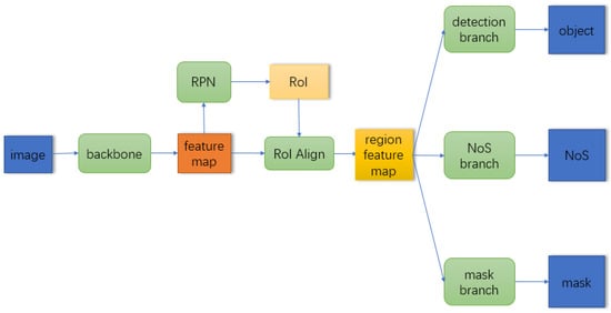
Figure 1.
Main architecture of NoS R-CNN. This figure is from [3].
2.2. Three Methods for GFA Estimation Based on the NoS R-CNN
We designed three GFA estimation methods based on NoS R-CNN, which are generated from different training and inference strategies in a unified network architecture in various degrees of end-to-end learning. The network architecture of the three proposed methods is shown in Figure 2. The proposed network adds both the BA branch and GFA branch (surrounded by the red dotted line in the Figure 2) based on NoS R-CNN for end-to-end BA and GFA prediction, respectively. The network architecture of both BA branch and GFA branch is consistent with the NoS branch, which is shown in Figure 3. Specifically, the NoS/BA/GFA branch takes the region feature of detected building objects as input. The region feature of detected building object will be further processed by two fully connected layers and the prediction of NoS/BA/GFA are outputted as a scalar. The three proposed methods are described in detail below.
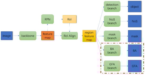
Figure 2.
Main network architecture of proposed methods.
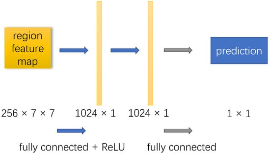
Figure 3.
Network architecture of BA branch and GFA branch. This figure is from [3].
2.2.1. Mask Branch-Based (MBB) GFA Estimation
This method only uses the detection, NoS, and mask branches in training and inference stage. The prediction of NoS branch is used as the NoS estimation, and the BA of building is obtained by calculating the number of building pixels which are predicted by the mask branch. The GFA prediction is obtained as follows:
where is the GFA prediction of this method, is the NoS prediction which is the output of NoS branch, is the number of positive pixels in segmentation mask which is the output of mask branch, is the ground area of a pixel.
2.2.2. BA Branch-Based (BABB) GFA Estimation
This method is similar to MBB and their difference is the way for BA acquisition. Specifically, detection, NoS, mask, and BA branch are used in training stage. The mask branch among them is only used for getting the auxiliary loss [17] and the other three branch also used in inference stage. The output of NoS branch is used as NoS prediction, and the output of BA branch is also used as the end-to-end BA estimation. The GFA prediction is obtained as follows:
where is the GFA prediction of this method, and are the output of NoS branch and BA branch, respectively.
2.2.3. GFA Branch-Based (GBB) GFA Estimation
Different from the above two methods, this method does not generate both the NoS and BA prediction in inference stage explicitly, but to make the end-to-end GFA prediction. Specifically, this method uses all the five branches in training stage, and the NoS, BA, and mask branches are used for getting the auxiliary loss. In inference stage, only detection and GFA branches are used, and the output of GFA branch is used as the final GFA prediction of the building detected by detection branch.
2.2.4. Training/Inference Strategies Comparison among Three Methods
In order to facilitate understanding the difference between the above three proposed methods, we show the training and inference strategies of those methods in Table 1. The symbol before/after “/” indicate the training/inference strategy of corresponding branch. For training strategy, “√” indicates the corresponding branch was trained in training stage and “×” indicates not. For inference strategy, “√” indicates the outputs of corresponding branch are used for instance-wise GFA prediction and “×” indicates not.

Table 1.
Training/Inference Strategies of three methods.
2.3. Loss Function and Implementation Details of Experiments
In this paper, NoS, BA, and GFA prediction are designed as regression tasks, so we use the smooth L1 function [18] which is often used in regression tasks as loss function for the added BA and GFA branch. The loss function for the above three regression tasks is:
where is the building objects in training set which have the NoS/BA/GFA ground truth (GT), is the number of building objects in , and , and are the GT and the prediction of building object i in . The total loss of the proposed three methods is:
where is the total loss of network, is the loss of Mask R-CNN. , and are losses of NoS, BA, and GFA branch, and, and are their weights.
Most of the experiment configurations and hyper-parameters are same as that in [3], such as batch size, learning rate, pretrain weight, etc. As a small number of buildings in our dataset have no NoS/GFA GT, they were not used for loss calculation or model evaluation for NoS/GFA task. The loss weight of NoS, BA, GFA branch in Equation (4) are shown in Table 2. It can be seen that the loss weight of BA and GFA branch is relatively small, especially for the GFA branch. This is because that the loss of corresponding branch is relatively large and we find that the loss on corresponding branch cannot be decreased unless using the small loss weight.
Table 2.
Loss weights configuration for three methods.
2.4. Dataset
We collected nine GF-2 images which are located at nine large cities in China, such as Beijing, Guangzhou, Xiamen, and so on. The PanSharp algorithm [19] was used to fuse the multispectral data with panchromatic band data, and its resolution was improved from 4 m to 1 m. Because all the images are almost orthomorphic, the building footprints are not shaded by other buildings and the side of buildings are invisible in images even for the high buildings, as shown in Figure 4. It also can be seen from Figure 4 that every building shadow cannot be extracted completely from image, so the traditional shadow-based NoS estimation method cannot be used in this scene. The building footprint contour vector data of the corresponding area was also collected and transformed into raster data which has the same spatial resolution as image data as instance segmentation GT. The bounding box and BA GT are obtained from the instance segmentation GT. Most of the building objects in our dataset have NoS GT, whose GFA GT are obtained by producing NoS and BA GT. We divided the images and the corresponding GT raster data into patches with the size of 256 × 256 without overlap as experimental samples, and randomly divided the samples into training set and test set, whose configuration are shown in Table 3. Figure 5 shows the geographical distribution of samples in the dataset. Figure 6a,b shows the distribution of number of buildings with different GFA on the training set and test set. Figure 6c,d shows distribution of number of buildings with different BA and NoS on the training set and test set.
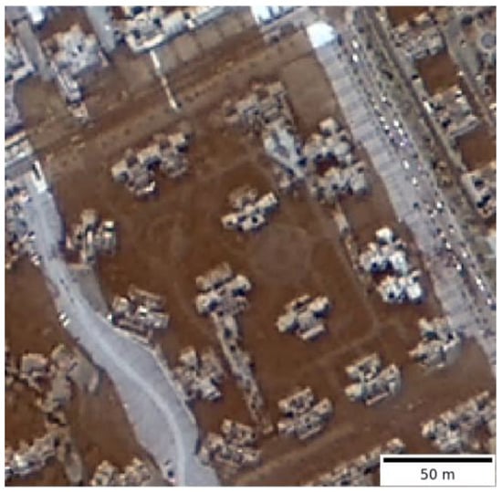
Figure 4.
Image in dataset for high buildings.
Table 3.
Configuration of dataset.
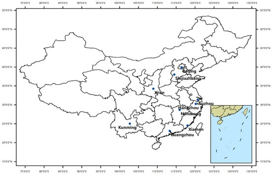
Figure 5.
The geographical distribution of images in the dataset. This figure is from [3].
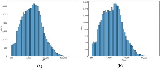
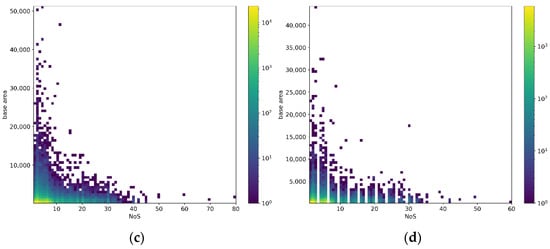
Figure 6.
Statistical distribution of samples in the dataset. (a) Distribution of GFA in training dataset. (b) Distribution of GFA in test dataset. (c) Joint distribution of NoS and base area in training dataset. (d) Joint distribution of NoS and area in test dataset.
3. Results
The goal of this paper is to design a method for instance-wise GFA estimation from monocular optical images, which consists of two tasks: detecting building objects and estimating the GFA of detected buildings. The building detection results are the carrier of the GFA estimation results. So, in practical scenarios, building objects detection accuracy and instance-wise GFA estimation accuracy are two determinants of the model performance. We will evaluate those two determinants in our experiment. For better understanding the performance of proposed methods, the results of MBB will be analyzed in detail.
3.1. Building Detection Task
We followed the evaluation method of building detection task in [3]. Specifically, the probability threshold was set to 0.5 for predicting the detected objects as building or not. The intersection over union (IoU) threshold was set to 0.5 for distinguishing the True Positive (TP), False Positive (FP), and False Negative (FN) samples. F1, precision and recall were used as evaluation metrics. Since the research focus of this paper is GFA estimation, not building object detection, the object detection method is directly based on the Mask R-CNN without any improvement. For evaluating the building detection performance of proposed methods accurately, we introduced the performance of vanilla Mask R-CNN on our dataset as the baseline of other methods. The building detection performances of those methods are shown in Table 4:
Table 4.
Building detection evaluation metrics (%).
From the Table 4, we can see that the detection performances of the proposed three methods are almost equal to that of the vanilla Mask R-CNN, even there is a little improvement on BABB.
3.2. GFA Estimation Task
We use the mean absolute error (MAE) and mean intersection over union (mIoU) in prediction mode A/B as the metrics for GFA estimation, which are referred from the evaluation methods for NoS estimation in [3]. The formula of MAE and mIoU are shown in Equations (5) and (6), where and are prediction and GT of the sample i, respectively. As the unit of the calculated value is maintained, MAE retains physical meaning and can be easily understood. The smaller the metric, the better the performance of the model performs. But MAE only takes account of the absolute error between prediction and GT, ignoring the relationship between the absolute error and corresponding GT. For example, the same absolute error is of different meaning for buildings with large GFA and small GFA. In this context, we introduced the mIoU which uses the form of ratio and considers the relationship between the predicted value and the true value. The larger the metric, the better the performance of the model performs. The metrics in mode A is for evaluating the performance of model in practical scenarios, and metrics in mode B is for accurately evaluating the difference of three proposed methods. Details of two prediction modes are described as follows.
In prediction mode A, images are inputted to the model, and the model outputs the building detection results and GFA estimation of detected buildings. Only TP samples of detected buildings were evaluated for GFA estimation. Because different objects might be detected by different models, the TP sample sets of different models are generally different. Consequently, models are evaluated on different building objects sets when using prediction mode A, showing that comparison of the different models is not strictly accurate. To address the problem, prediction mode B is introduced, where images and bounding box GT of all the building objects in test set are inputted into the model, and the model outputs the GFA estimation of the given building objects. Different methods are evaluated on the same building objects set and share the same bounding box GT, excluding the influence of detection results on GFA estimation. The performance of three proposed methods on GFA estimation task are shown in Table 5, where “@ TP” and “@ all” end with the evaluation of the prediction results of mode A and mode B, respectively.
Table 5.
GFA estimation evaluation metrics.
From Table 5, we can see that for prediction mode A, MBB is obviously better than BABB and GBB on MAE. The performance of all the three methods are very close in terms of mIoU. For prediction mode B, MBB is obviously better than the other two methods in terms of both MAE and mIoU. The BABB is a little better than GBB.
3.3. Further Analysis for the Results of MBB
As MBB is the best methods among the proposed three methods, we show the prediction of MBB in mode A on six patches in test set in Figure 7 and their metrics in Table 6 for better understanding the performance of the proposed methods for GFA estimation. Considering that GFA is difficult to be visualized and MBB predicts GFA by separately estimating NoS and segmenting the building footprints, the results of NoS estimation and footprints segmentation are shown for intuitively linking the reported metrics and the performance of the model.
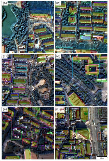
Figure 7.
Prediction result of MBB in mode A. There are six subfigures (a–f), which correspond to six selected patches, respectively. Each subfigure shows the “TP”, “FP”, and “FN” prediction of MBB in mode A. The color of the bounding boxes has no specific meaning, just in order to distinguish different building instance. Most bounding boxes have a pair of numbers separated by “|”. For TP samples, the first number is the NoS prediction of the model and the second is the NoS GT. The bounding boxes with pairs start with “FP”/“FN” are “FP”/”FN” objects and the numbers of those are predicted/true NoS. All predicted values shown in the figure have been rounded up or rounded down to the nearest decimal. For example, a bounding box with the label “4|6” indicates that the bounding box is the prediction of a “true positive” sample whose NoS prediction and ground truth is 4 and 6, respectively. A bounding box with the label “FP|3” indicates that the bounding box is the prediction of a “false positive” sample whose NoS prediction is 3. A bounding box with the label “FN|1” indicates that the bounding box is the ground truth of a “false negative” sample whose NoS ground truth is 1. For every TP sample, the TP/FP/FN pixels of segmentation are shown in transparent yellow/red/green.
Table 6.
Metrics of six test patches of MBB in mode A. The first/second column shows the MAE of BA/NoS estimation performance. The third/fourth column shows the MAE/mIoU of GFA estimation performance.
For the performance of detection task, it can be seen from Figure 7 that there are several FP/FN samples, which indicate that the performance of detection task should be improved, especially for the small buildings. There are a few buildings in which complex structure are detected as several separated buildings in Figure 7c,e which indicate the approach that detecting buildings from 1 m spatial resolution satellite images deserves to be improved furthermore. For NoS estimation, the performance is generally acceptable for low buildings and unstable for high buildings. This problem was discussed in detail in [3] and has not been addressed very well up to now. For the building footprints segmentation, the main structures of most buildings have been segmented, but the boundaries of prediction are not precisely aligned with the ground truth, especially for the buildings with complex boundaries. For GFA estimation task, it can be seen from Table 6 that there is a large range for MAE from 752 to 4018, which indicate that the absolute error of the model varied largely depending on the scenes. With respect to mIoU whose values fluctuate around 0.8, it can be roughly inferred that there is an uncertainty of about 20 percent for the GFA estimation of every building, which can also be inferred from the performance of NoS estimation and footprints segmentation results shown in Figure 7.
Based on the above analysis, two conclusions can be drawn:
- As GFA estimation using MBB can be divided into three subtasks, i.e., building detection, NoS estimation and building footprints segmentation, the performance of GFA estimation can be improved by improving the three subtasks. The performance of building detection task and footprints segmentation task can be improved by any methods which are helpful for instance segmentation, such as using updated and more powerful base networks or backbones. The performance of NoS estimation is of vital importance to the performance of GFA estimation, especially for the buildings with large BA whose errors of GFA are more easily amplified by the errors of NoS prediction. But accurate NoS estimation from monocular optical satellite images is not widely studied and is still an open question. We believe that the shadows of buildings in the images are helpful for improving the performance of NoS estimation, but the efficient methods to use this information need to be studied furthermore.
- It can be seen from Table 5 and Figure 7 that the accuracy of the proposed method is still promising for GFA estimation. Although the capability of model deserves being improved furthermore, the task itself, i.e., estimating instance-wise GFA from monocular optical satellite images, is still a challenging problem. Compared with LiDAR or optical stereo images, the available information of monocular optical images is limited, especially for the NoS estimation task, which can be verified in Figure 7. Besides, the proposed methods should not rely only on the specific feature, e.g., the shadow of buildings, so that it can be applied in a wide range, including the complex scenarios. In view of the above, the proposed methods are valuable for applications for which the very high accuracy is not necessary because the users of the model should take into consideration the tradeoff between the accuracy and the generality of model as well as the cost.
- Due to land resources limitations, rapid urbanization causes urban expansion not only in 2-dimension (2-D), but also in 3-dimension (3-D), especially in China [20,21]. Due to the difficulty of the large-scale 3-D data acquisition, most of the geographical analyses such as population density estimation [22,23,24], heat island intensity [25,26], and geology–environmental capacity [27] for large scale are based on 2-D information. Although the results of the above applications can be partially inferred from the 2-D building coverage distribution, some errors are inevitable due to the ignored information in the vertical direction, and the error will be increased along with the rapid urban expansion in 3-D. Although the capability of model deserves being improved furthermore, the results of the proposed methods can reduce the error to some extent for the applications based on 2-D information. For example, the GT of BA and the mean value of NoS can be used for all the building instances to estimate GFA, which simulate the methods only using the 2-D information, whose mIoU is 0.566 on our test set. Compared with the above method, the proposed MBB whose mIoU is 0.683 reduced about 20 percent error for every building instance on average even though the GT of BA were not used for MBB.
4. Discussion
4.1. Comparison of Three Proposed GFA Estimation Methods
According to the definition of GFA, the performances of NoS and BA estimation are directly related to the performance of GFA estimation. In order to explore the difference of performances between three proposed methods, we analyzed the difference of performances for both NoS and BA estimation tasks. The GFA prediction of MBB and BABB depends on the prediction of both NoS and BA in inference stage, which can be obtained explicitly and are used for evaluating the performance of BA and NoS estimation for MBB and BABB. NoS and BA prediction are not necessary for GFA estimation of GBB in inference stage but are used in training stage to get the auxiliary loss for improving GFA estimation. Here the outputs of BA and NoS branch of GBB in inference stage are used for evaluating the performance of BA and NoS estimation of GBB. We use MAE in prediction mode A/B as metric in this section, and the performances of the three methods are shown in Table 7, where “NoS”/“BA” indicate the NoS/BA estimation task.
Table 7.
NoS and BA estimation evaluation metrics.
We discuss MBB and BABB first. For mode A, the performances on BA estimation between MBB and BABB are close, but MBB is better in NoS estimation. So, the stronger ability of MBB for NoS estimation may be the reason for better performance in GFA estimation in mode A. For mode B, although MBB is worse than BABB on NoS estimation, but obviously better on BA estimation. The great advantage of MBB on BA estimation may be the reason for better performance on GFA estimation in mode B.
Then we discuss BABB and GBB. For mode A, the performances of GBB on NoS and BA estimation tasks are worse than BABB, but the gap is not so large. So, the performances of the two methods on GFA estimation task are close. For mode B, the performances of the two methods on BA estimation are basically consistent, but BABB is better than GBB on NoS estimation. Therefore, the better performance of BABB on NoS estimation may be the reason for better performance in GFA estimation in mode B.
It can be seen that NoS branches were trained identically for three methods, i.e., using the same loss weight, network architecture, and other hyper-parameters. However, their performances are different as for NoS estimation task. The possible reason might be that the total loss of multitasks are different for three methods, and the loss of different tasks can be influenced by each other. The same reason can also be applied for explaining the performance differences for BA estimation tasks between BABB and GBB.
4.2. Comparison between the Two BA Estimation Methods
The way for BA estimation is the main difference of BABB and MBB. For the BA estimation task, BABB follow the end-to-end fashion and MBB not. For further comparing the performances of BA estimation methods of both BABB and MBB, we plot the joint distribution of prediction and GT of BA in Figure 8, which is consisted of four subfigures. The left/right column shows the results of MBB/BABB, and the top/bottom row of subfigures shows the results in prediction mode A/B. We plot the line y = x in subfigures, in which the closer the points are, the less prediction errors the points have. It can be seen that prediction and GT show positive correlation in all four subfigures, and the shapes of distributions are roughly symmetrical along the y = x. For buildings with small BA, the error is also small. With the increase of BA, the number of predictions with large error is increasing. From the Figure 8a,b, it can be seen that the distributions of MBB and BABB in mode A are generally the same, which is consistent with the results in Table 7. From the Figure 8c, it can be seen that there are many underestimated predictions with small BA for MBB. It may be because buildings with small BA are relatively difficult to be completely detected for segmentation, which leads to the underestimation for BA. The same situation can also be found but not obvious for mode A, this may be because that there are less buildings with small BA in TP samples because of the difficulty for small BA building detection. The underestimation mentioned above mainly appears on small BA buildings, whose error are generally small, so it does not lead to large MAE. From the Figure 8d, it can be seen that the underestimation mentioned above is not obvious for BABB, but the predictions of BABB are more scattered, especially for the buildings with large BA, which leads to relatively larger errors. So, the performance of BABB is worse than MBB for MAE.
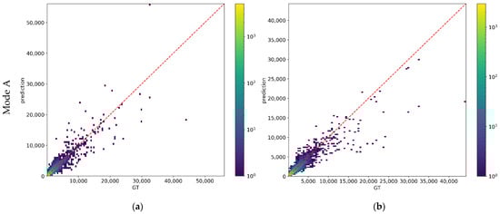
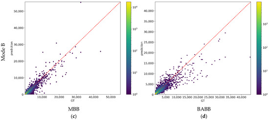
Figure 8.
Joint distribution of prediction and GT of BA. (a) The results of MBB in mode A. (b) The results of BABB in mode A. (c) The results of MBB in mode B. (d) The results of BABB in mode B. y = x is plotted in red in each subfigure.
4.3. End-to-End Fashion Is Not a Panacea
Compared with the traditional machine learning methods which depended on the hand-designed features or individual component modules, one of the most prominent advantages of deep learning is its inherent feature engineering capability based on the end-to-end learning. Many research [28,29,30] showed the performance advantages of end-to-end design compared with non-end-to-end design and successes on novel tasks which are very difficult to be realized without end-to-end models, such as height estimation task from monocular images [31,32,33]. In order to take full advantage of end-to-end design, three GFA estimation methods proposed in this paper use the end-to-end design in various degrees. For BA estimation task, BABB directly predicts BA from region feature, whereas MBB segment footprint then transforms it to BA. So, the degrees of end-to-end learning between the two methods is BABB > BA. For GFA estimation task, GBB directly predicts GFA from region feature whereas both BABB and MBB need to extract BA and NoS separately before obtaining GFA. Considering the above analysis, the degrees of end-to-end learning for the three proposed methods can be given as: GBB > BABB > MBB. BABB and BA which separately extract BA and NoS depend on the accuracy of both the subtasks. These two less end-to-end designed methods have larger risk of bad performance than GBB intuitively because large error of either of two subtasks will lead to bad performance of final results. According to experiment results in this paper, for both GFA and BA estimation task, there is an inverse relationship between model performance and degree of end-to-end learning. This result indicates that the more end-to-end design may be not the best choice for GFA and BA estimation tasks and not always better than less end-to-end design in any circumstance. We analyze the possible reason of the poor performance for the more end-to-end designed methods compared to the less ones in our experiments as follows:
- Insufficient training data. Compared with the less end-to-end designed model, the more end-to-end designed methods generally rely on more training data for the satisfactory performance because of their data-driven mechanism. Although the training data used in our experiment is much more than that used in the previous research, yet it may be insufficient for the more end-to-end designed models to give full play to their advantages.
- Inappropriate model design. Because this paper is the first attempt to directly estimate instance-wise GFA end-to-end using deep convolutional neural network to the best of our knowledge, there are not any model designs for reference. We basically follow the detection task pipeline inspired by the Mask R-CNN for GFA/BA prediction. This design may not be appropriate for GFA/BA estimation task. Or may be the more end-to-end model design is inappropriate for GFA/BA estimation task in nature.
4.4. Is the CNN Irreplaceable for This Task?
With the help of deep learning, CNN has achieved great success in many image processing tasks, such as semantic segmentation and object detection. In this paper, we attempted to use the three CNN-based methods to achieve the task of GFA estimation. There is a valuable question, is it possible to achieve the comparable performance for the GFA estimation task using the more lightweight model without CNN. To answer this question, two popular traditional regression models using the hand-craft feature, i.e., the multi-layer perception (MLP) and the random forest (RF), were introduced in the experiments in this section to answer this question.
The implementation of the above two methods are based on [34]. For MLP, 5 hidden layers with 100 neurons of each layer were used. For RF, 100 trees whose depth were less than 10 were used. Other hyper parameters of the above two methods were kept with the default setting in [34]. The dataset used in this section was kept with that in Section 2.4. The hand-craft feature for every building insurance are described as follows: for every building instance, the segmentation GT of building footprint was used as the inner mask and the inner masks were dilated by 10 pixels to get the outer mask. The inner mask was used to extract the mean value and the standard deviation of every channel of the inputted image, then a feature vector with 6 elements was obtained as the inner feature of building instance. The outer feature can be obtained by using the outer mask to extract the feature of instance like the inner feature. The diagram of inner mask and outer mask is shown in Figure 9. The inner and outer feature were concatenated and finally a feature vector with 12 elements was obtained as a feature of every building instance for the MLP and the RF. The performances of the CNN-based models proposed in this paper and the two traditional methods mentioned above using the hand-craft feature are shown in Table 8. In Table 8, CNN, MLP, and RF estimated GFA by separately extracting BA and NoS. CNN-ETE, MLP-ETE, and RF-ETE estimated GFA based on the instance feature in an end-to-end (ETE) manner.
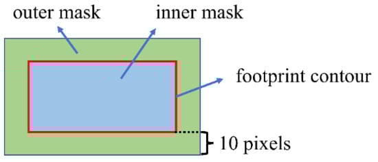
Figure 9.
Diagram of inner mask and outer mask.
Table 8.
Metrics of CNN, MLP, and RF on test set.
From Table 8, it can be seen that:
- The CNN-based methods show much better performance than MLP and RF on the BA, NoS and GFA estimation tasks. These results indicate that the tradition methods using the hand-craft features, i.e., MLP and RF, might be not suitable for these difficult tasks which are even extremely hard for ordinary people to achieve because of the limited information on NoS in monocular optical satellite images. Although the CNN-based methods seem to be more cumbersome, they indeed showed the irreplaceable capability because of its data-driven mechanism.
- The performance of MLP in an end-to-end manner (MLP-ETE) is better than the MLP, which showed inconsistent conclusions for CNN-ETE and CNN. These results further showed the necessity and the value of experiments described in Section 3.2 for comparing the performance of the proposed three methods.
5. Conclusions
In this paper, three instance-wise GFA estimation methods from monocular optical images are proposed for the first time, i.e., MBB, BABB, GBB. These three methods are based on NoS R-CNN and use the end-to-end design in various degrees. Compared with the existing GFA estimation methods, the proposed methods are low-cost, universal, and flexible. Experiments on our dataset from nine large cities in China were carried out in order to compare the performances of the three proposed methods. The results show that the building detection performances of the proposed three methods are almost equal to vanilla Mask R-CNN and the GFA estimation performance ranking is MBB > BABB > GBB, which is the reverse order of degrees of end-to-end learning of three methods. Results are analyzed in detail for exploring the reasons for the performance gap between the three methods, and we think that the more end-to-end designed methods are more difficult for BA/GFA estimation tasks. The quantitative and qualitative evaluations of the proposed methods indicate that the performances of proposed methods for accurate GFA estimation are promising for potential applications using large-scale remote sensing images. It will consume large cost in time, labor, and economy for the large-scale instance-wise GFA acquisition. With the development of remote sensing technique, the high resolution monocular optical satellite images have become more and more convenient to be obtained. Although the stereo images-based methods or shadow-based method can be used for GFA acquisitions, those methods cannot be applied in a wide range due to the high data acquisition cost or inherent defect of methods. Based on the methods proposed in this paper, the models can be trained on the existing data, then to be applied to the large-scale area without GFA information from the monocular optical satellite images to get the instance-wise GFA information in a rapid, cost-effective manner. We hope that this paper can provide new perspectives on related approaches and downstream tasks.
Author Contributions
Conceptualization, H.T.; funding acquisition, H.T.; investigation, H.T. and C.J.; methodology, C.J.; software, C.J.; and supervision, H.T. All authors have read and agreed to the published version of the manuscript.
Funding
This work was supported in part by the National Natural Science Foundation of China under Grant No. 41971280.
Institutional Review Board Statement
Not applicable.
Informed Consent Statement
Not applicable.
Data Availability Statement
Not applicable.
Conflicts of Interest
The authors declare no conflict of interest.
References
- Yang, N.; Tang, H. Semantic Segmentation of Satellite Images: A Deep Learning Approach Integrated with Geospatial Hash Codes. Remote Sens. 2021, 13, 2723. [Google Scholar] [CrossRef]
- Huang, W.; Tang, H.; Xu, P. OEC-RNN: Object-oriented delineation of rooftops with edges and corners using the recurrent neural network from the aerial images. IEEE Trans. Geosci. Remote Sens. 2021, 60, 5604912. [Google Scholar] [CrossRef]
- Ji, C.; Tang, H. Number of Building Stories Estimation from Monocular Satellite Image Using a Modified Mask R-CNN. Remote Sens. 2020, 12, 3833. [Google Scholar] [CrossRef]
- Frantz, D.; Schug, F.; Okujeni, A.; Navacchi, C.; Wagner, W.; van der Linden, S.; Hostert, P. National-scale mapping of building height using Sentinel-1 and Sentinel-2 time series. Remote Sens. Environ. 2021, 252, 112128. [Google Scholar] [CrossRef]
- Cao, Y.; Huang, X. A deep learning method for building height estimation using high-resolution multi-view imagery over urban areas: A case study of 42 Chinese cities. Remote Sens. Environ. 2021, 264, 112590. [Google Scholar] [CrossRef]
- Wang, C.; Ma, J.; Liang, F. Floor Area Ratio extraction based on Airborne Laser Scanning data over urban areas. In Proceedings of the 2010 IEEE International Geoscience and Remote Sensing Symposium, Honolulu, HI, USA, 25–30 July 2010; pp. 1182–1185. [Google Scholar]
- Roca Cladera, J.; Burns, M.; Alhaddad, B.E. Satellite Imagery and LIDAR Data for Efficiently Describing Structures and Densities in Residential Urban Land Use Classification. Remote Sens. Spat. Inf. Sci. 2013, XL-4/W1, 71–75. [Google Scholar]
- Wu, Q.; Chen, R.; Sun, H.; Cao, Y. Urban building density detection using high resolution SAR imagery. In Proceedings of the 2011 Joint Urban Remote Sensing Event, Munich, Germany, 11–13 April 2011; pp. 45–48. [Google Scholar]
- Wen, D.; Huang, X.; Zhang, A.; Ke, S. Monitoring 3D building change and urban redevelopment patterns in inner city areas of Chinese megacities using multi-view satellite imagery. Remote Sens. 2019, 11, 763. [Google Scholar] [CrossRef]
- Peng, F.; Gong, J.; Wang, L.; Wu, H.; Yang, J. Impact of Building Heights on 3D Urban Density Estimation from Spaceborne Stereo Imagery. Int. Arch. Photogramm. Remote Sens. Spat. Inf. Sci. 2016, 41, 677–683. [Google Scholar]
- Zhang, X.; Chen, Z.; Yue, Y.; Qi, X.; Zhang, C.H. Fusion of remote sensing and internet data to calculate urban floor area ratio. Sustainability 2019, 11, 3382. [Google Scholar] [CrossRef]
- Zhang, X. Village-Level Homestead and Building Floor Area Estimates Based on UAV Imagery and U-Net Algorithm. ISPRS Int. J. Geo-Inf. 2020, 9, 403. [Google Scholar] [CrossRef]
- Duan, G.; Gong, H.; Liu, H.; Yi, Z.; Chen, B. Establishment of an Improved Floor Area Ratio with High-Resolution Satellite Imagery. J. Indian Soc. Remote Sens. 2018, 46, 275–286. [Google Scholar] [CrossRef]
- Wu, Y.Z.; Li, B. Estimating Floor Area Ratio of Urban Buildings Based on the QuickBird Image. Advanced Materials Research; Trans Tech Publications Ltd.: Freienbach, Switzerland, 2012; Volume 450, pp. 614–617. [Google Scholar]
- Yan, M.; Xu, L. Relationship Model between Nightlight Data and Floor Area Ratio from High Resolution Images. Int. Arch. Photogramm. Remote Sens. Spat. Inf. Sci. 2017, 42, 1419–1422. [Google Scholar] [CrossRef][Green Version]
- Zhang, F.; Du, B.; Zhang, L. A multi-task convolutional neural network for mega-city analysis using very high resolution satellite imagery and geospatial data. arXiv 2017, arXiv:1702.07985. [Google Scholar]
- He, K.; Gkioxari, G.; Dollár, P.; Girshick, R. Mask r-cnn. In Proceedings of the IEEE International Conference on Computer Vision, Tokyo, Japan, 13–17 March 2017; pp. 2961–2969. [Google Scholar]
- Girshick, R. Fast r-cnn. In Proceedings of the IEEE International Conference on Computer Vision, Las Condes, Chile, 11–18 December 2015; pp. 1440–1448. [Google Scholar]
- Sun, W.; Chen, B.; Messinger, D. Nearest-neighbor diffusion-based pan-sharpening algorithm for spectral images. Opt. Eng. 2014, 53, 013107. [Google Scholar] [CrossRef]
- Liu, M.; Ma, J.; Zhou, R.; Li, C.; Li, D.; Hu, Y. High-resolution mapping of mainland China’s urban floor area. Landsc. Urban Plan. 2021, 214, 104187. [Google Scholar] [CrossRef]
- Cao, Q.; Luan, Q.; Liu, Y.; Wang, R. The effects of 2D and 3D building morphology on urban environments: A multi-scale analysis in the Beijing metropolitan region. Build. Environ. 2021, 192, 107635. [Google Scholar] [CrossRef]
- Kono, T.; Kaneko, T.; Morisugi, H. Necessity of minimum floor area ratio regulation: A second-best policy. Ann. Reg. Sci. 2010, 44, 523–539. [Google Scholar] [CrossRef]
- Wu, S.; Qiu, X.; Wang, L. Population estimation methods in GIS and remote sensing: A review. GISci. Remote Sens. 2005, 42, 80–96. [Google Scholar] [CrossRef]
- Wang, L.; Wu, C. Population estimation using remote sensing and GIS technologies. Int. J. Remote Sens. 2010, 31, 5569–5570. [Google Scholar] [CrossRef]
- Sultana, S.; Satyanarayana, A.N.V. Urban heat island intensity during winter over metropolitan cities of India using remote-sensing techniques: Impact of urbanization. Int. J. Remote Sens. 2018, 39, 6692–6730. [Google Scholar] [CrossRef]
- Shirani-Bidabadi, N.; Nasrabadi, T.; Faryadi, S.; Larijani, A.; Roodposhti, M.S. Evaluating the spatial distribution and the intensity of urban heat island using remote sensing, case study of Isfahan city in Iran. Sustain. Cities Soc. 2019, 45, 686–692. [Google Scholar] [CrossRef]
- Cui, Z.-D.; Tang, Y.-Q.; Yan, X.-X.; Yan, C.-L.; Wang, H.-M.; Wang, J.-X. Evaluation of the geology-environmental capacity of buildings based on the ANFIS model of the floor area ratio. Bull. Eng. Geol. Environ. 2010, 69, 111–118. [Google Scholar] [CrossRef]
- Ren, S.; He, K.; Girshick, R.; Sun, J. Faster R-CNN: Towards Real-Time Object Detection with Region Proposal Networks. IEEE Trans. Pattern Anal. Mach. Intell. 2017, 39, 1137–1149. [Google Scholar]
- Tao, A.; Sapra, K.; Catanzaro, B. Hierarchical multi-scale attention for semantic segmentation. arXiv 2020, arXiv:2005.10821. [Google Scholar]
- Yu, J.; Lin, Z.; Yang, J.; Shen, X.; Lu, X.; Huang, T. Free-form image inpainting with gated convolution. In Proceedings of the IEEE/CVF International Conference on Computer Vision, Seoul, Korea, 27–28 October 2019; pp. 4471–4480. [Google Scholar]
- Amirkolaee, H.A.; Arefi, H. Height estimation from single aerial images using a deep convolutional encoder-decoder network. ISPRS J. Photogramm. Remote Sens. 2019, 149, 50–66. [Google Scholar] [CrossRef]
- Ghamisi, P.; Yokoya, N. IMG2DSM: Height simulation from single imagery using conditional generative adversarial net. IEEE Geosci. Remote Sens. Lett. 2018, 15, 794–798. [Google Scholar] [CrossRef]
- Srivastava, S.; Volpi, M.; Tuia, D. Joint height estimation and semantic labeling of monocular aerial images with CNNs. In Proceedings of the 2017 IEEE International Geoscience and Remote Sensing Symposium (IGARSS), Fort Worth, TX, USA, 23–28 July 2017; pp. 5173–5176. [Google Scholar]
- Pedregosa, F.; Varoquaux, G.; Gramfort, A.; Michel, V.; Thirion, B.; Grisel, O.; Blondel, M.; Prettenhofer, P.; Weiss, R.; Dubourg, V.; et al. Scikit-learn: Machine learning in Python. J. Mach. Learn. Res. 2011, 12, 2825–2830. [Google Scholar]
Publisher’s Note: MDPI stays neutral with regard to jurisdictional claims in published maps and institutional affiliations. |
© 2022 by the authors. Licensee MDPI, Basel, Switzerland. This article is an open access article distributed under the terms and conditions of the Creative Commons Attribution (CC BY) license (https://creativecommons.org/licenses/by/4.0/).