An Object-Oriented Approach to the Classification of Roofing Materials Using Very High-Resolution Satellite Stereo-Pairs

Abstract

The availability of multispectral images, with both high spatial and spectral resolution, makes it possible to obtain valuable information about complex urban environment, reducing the need for more expensive surveying techniques. Here, a methodology is tested for the semi-automatic extraction of buildings and the mapping of the main roofing materials over a urban area of approximately 100 km², including the entire city of Bologna (Italy). The methodology follows an object-oriented approach and exploits a limited number of training samples. After a validation based on field inspections and close-range photos acquired by a drone, the final map achieved an overall accuracy of 94% (producer accuracy 79%) regarding the building extraction and of 91% for the classification of the roofing materials. The proposed approach proved to be flexible enough to catch the strong variability of the urban texture in different districts and can be easily reproducible in other contexts, as only satellite imagery is required for the mapping.

1. Introduction

The WorldView-3 (WV3) satellite platform offers unprecedented capabilities of very high spectral and spatial resolution. It provides a 0.3 m resolution panchromatic sensor, an eight-band visible and near-infrared imager (operating between 397 and 1039 nanometres) with a ground sample distance (GSD) of 1.2 m, a short-wave infrared (SWIR) sensor with further eight bands (1184—2373 nm) at a resolution of 3.7 m, and finally the CAVIS (Clouds, Aerosol, Vapors, Ice, and Snow) sensor with twelve additional bands at 30 m for the retrieval of atmospheric properties [1]. These capabilities make it particularly suitable for application in urban areas, where the extremely complex morphology requires a higher level of detail [2,3].

The present paper proposes an approach for the detection of buildings and the classification of the major roofing material types entirely based on the satellite WV3 data, without any ancillary information. This method is tested over an area of approximately 100 km², covering an entire city, and aims to be easily repeatable in most of the urban contexts, as the only required data are the satellite images.

Automatic building detection from remote sensing has been widely debated in the scientific literature and a detailed review is beyond the scope of the present paper. Readers are referred to recent review papers [4,5,6]. Here, only contributions where the classification of roofing materials is considered (alongside the problem of roof detection) are briefly discussed. This problem has been addressed for several purposes, encompassing building inventory for earthquake damage assessment [7], identification of hazardous materials such as asbestos [8,9], and for thermal flux or energy efficiency studies that require proper determination of surface emissivity in a smart city perspective [10,11], among others.

It is to be noted that very often the published tests are performed over very limited areas (typically a few square kilometers) [12,13,14], with relatively homogeneous urban texture. From the point of view of the main data sources, two approaches were proposed in the literature: the first relies only on images, which can be multispectral [8,9,15] or hyperspectral [16,17,18], and the second combines images with a digital elevation model of the urban area [14,19]. When included in the processing, the contribution of the elevation model becomes dominant especially for the identification of roof surfaces (by excluding all the other urban elements), while spectral information is used for material identification [19]. Although some spectral libraries of building materials were developed recently [20,21], classification approaches based on training samples or on decision rules are often preferred, especially with multispectral data [13,19].

When working on images only, the classification process is based on the spectral content and requires both a high spatial and spectral resolution. Moreira and Galvão [16] found that near and short-wave infrared bands provide the best discrimination, when using MIVIS data and field spectral signatures as training for the spectral angle mapper classifier. Better results in terms of overall accuracy (up to 97%) were achieved with machine learning algorithms, such as support vector machine (SVM) and random forest [17], or convolutional neural network [22].

A recent work by Kim et al. [23] implemented deep learning algorithms using aerial images with four bands only, but it was limited to a few materials (concrete and metal) and required an extensive training dataset (more than 11,600 images). Usually, when working with multispectral sensors (with a more limited number of bands compared to hyperspectral ones), images are to be coupled with elevation information and an object-oriented approach is to be preferred, in order to achieve comparable accuracy levels [12,15]. Abriha et al. [15] also tested the application of pan-sharpening to WorldView-2 imagery, to investigate possible benefits in terms of accuracy, and found improvements by 2–3% with some drawbacks in shadowed areas.

In all the proposed approaches multispectral images and elevation data come from different sources; usually, digital elevation models come from LiDAR surveys, which are not available everywhere and are expensive [24]. For this reason, the present work proposes an approach entirely based on satellite stereo-pairs, which can provide both spectral and elevation information with lower costs and widespread availability.

The adopted classification strategy is based on OBIA (Object-Based Image Analysis) techniques [25,26]. OBIA refers to classification approaches that investigate geographic entities or phenomena delineating and analyzing image objects rather than pixels [27]. OBIA emerged as particularly useful for extracting and mapping features from high spatial resolution images [28]. OBIA involves two main steps: segmentation and classification. The segmentation phase divides the image into objects, i.e., homogeneous groups of contiguous pixels that have similar spectral and/or spatial characteristics [29]. The segmentation step can be performed in a hierarchical approach, with semantic relationships between objects at different levels [30]. The classification is therefore based on the different spectral, shape, texture, hierarchical, and contextual features of these objects [31].

The validation of OBIA classifications is still debated in the literature and, even though several approaches have been proposed, there is not an obvious solution [32]. The optimal choice depends on the types of OBIA application, which can span from a complete partition of the studied area into polygons to the detection or delineation of selected spatial entities [33]. The confusion matrix, usually expressed in terms of areas or feature count, provides valuable information, even if it is not sufficient to fully characterize the quality of the obtained products [34]. In theory, the geometric quality of the segmentation should be assessed in terms of both location and shape. Many metrics can be defined to evaluate the similarity of mapped polygons against reference polygons, but most of them assume a one-to-one correspondence that is unlikely or even impossible to achieve in many applications, due to under or over-segmentation. This problem can be overcome by identifying corresponding polygons on the basis of intersection criteria, but their practical implementation varies greatly in the published works.

This paper adopts a separate assessment for the segmentation phase (mainly related to the problem of building identification) and the thematic accuracy of the obtained roofing materials map. The computation of the confusion matrix is adapted to handle the problem of over-segmentation.

2. Materials

The study area is the entire city of Bologna (Italy), which includes very different kinds of urban texture. The city center is mainly composed of a dense pattern of historical buildings and small houses with complex shapes and narrow streets, characterized also by the typical porticoes that became UNESCO World Heritage in 2021 [35]. Conversely, in the peripheral and productive districts a wider variety of building types can be found (e.g., industrial sheds and condominiums), and many open spaces are present. The terrain has a mainly flat topography, with an average elevation of 60 m a.s.l., except for the southern part that includes a hillside, with moderate slopes, higher vegetation coverage and far lower building density.

Three WV3 panchromatic stereo-pairs were acquired (one on 14 September 2017 and two on 20 September 2017); furthermore, two multispectral and SWIR images were also acquired (20 September 2017). Overall, they cover an area of approximately 100 km² (including all the urbanized territory of the municipality, see Figure 1) and can be considered cloud-free and haze-free. All the images were partially preprocessed by the supplier at the Ortho-Ready level.

For the orthorectification purpose, five ground control points were measured using network real-time kinematic (NRTK) techniques, based on virtual reference stations, with a precision of the measured coordinates of ~2 cm. Furthermore, to perform the atmospheric correction, four spectral signatures of different land cover materials were measured in the field (contemporary to image acquisition) with an SVC HR-768i portable spectroradiometer, and properly georeferenced with NRTK measurements.

For validation purposes, the technical cartography (TC) of the municipality, which comes with a nominal scale of 1:2000 and a tolerance for planimetric coordinates of ~0.5 m, was used to create the ground truth polygons and handle the over-segmentation problems. The cartography is updated to autumn 2016.

All the data were coherently framed in the ETRF2000 (epoch 2008), which is the official geodetic framework for Italy.

To validate the classification, several field data were acquired during dedicated surveys by directly accessing some roofs and using also the information derived by some inspections using UAVs (Unmanned Aerial Vehicles).

2.1. UAV Inspections

Video inspection using a drone was chosen to expand the calibration and validation dataset. Sequences of close-range images were acquired above the surveyed buildings, in order to unequivocally recognize the material of the inspected roofs.

The area analyzed for this project is an urban center and consequently strict restrictions are placed on UAV flights, for the protection of sensitive areas (such as airports and buildings of strategic importance) and to ensure the safety of the population living in densely inhabited area. These restrictions impose a maximum flight altitude above the ground level: it varies from 0 m (No Fly Zone) in the immediate vicinity of the sensitive areas, to 25 and 45 m moving away from them. In most of the city area the limit is 60 m. These limitations were considered in the design of the overflights, as it was necessary to avoid the no-fly zones and also the areas with the 25 m limit, as it is penalizing for roof inspections of tall buildings. Furthermore, the requirement to operate in “visual line of sight” (the pilot never loses sight on the drone) and to prevent interferences on the radio control results in a maximum horizontal distance between the UAV and pilot of 100 m. This implied the need to perform numerous take-offs and landings to inspect sufficiently large portions of the territory.

A small UAV was chosen, with a take-off weight of less than 0.25 kg. It mounts a 12 megapixel optical sensor installed on a gimbal, to allow precise orientation of the camera controlled by remote. Given the equivalent focal length of 25 mm and a maximum flight height of 45 m, the resulting GSD is no wider than 0.02 m.

Because of the premises described above, it was therefore not possible to follow rigorous statistical criteria for the random selection of the sampling points, but these overflight areas necessarily had to fall within those where aerial activity is permitted. Despite these limitations, four areas with heterogeneous roofing were carefully chosen to maximize the amount of information obtained. Overall, 12 fights were performed over these four areas, covering ~0.5 km² in total.

3. Methods

3.1. DSM Extraction

The procedure for the generation of the DSM is already discussed in the technical note in [2], and only the most relevant features are recalled here. The entire photogrammetric process was performed in the OrthoEngine tool of the Geomatica suite (version 2018, PCI Geomatics, Markham, ON, Canada), using a matching strategy based on the semi-global matching technique [36]. The WV3 images were oriented through a rational polynomial model, using the coefficient provided by the supplier. The model was further refined with a first-order polynomial, whose coefficients were estimated using five control points and 73 tie-points, well distributed in the study area and manually collimated. The overall root mean square error (RMSE) of the residuals was well below one pixel. The DSM extraction was performed with the highest possible resolution, which is the original resolution of the panchromatic band (0.3 m), and no smoothing filters were applied. The DSM was validated with check points and existing models of the area (from LiDAR data and oblique aerial images). Roof surfaces and open spaces are reconstructed with an average error of 1–2 pixels, but severe discrepancies frequently occur in narrow roads and urban canyons (up to several meters in average) [2].

For the present work, the DSM was further processed to remove the elevation of buildings and trees and estimate a DTM. Considering the peculiarity of the urban environment, where built-up surfaces cover most of the area, DTM computation was based on a percentile filter applied on the raster DSM. A large square kernel (300 pixels, equal to 90 m) was considered, in order to include enough pixels at the terrain level. The 10-percentile of the elevation values was computed inside each kernel and assumed as the terrain level, excluding possible outliers due to some residual noise in the model. Considering the overlap of 50% between adjacent kernels, the final DTM comes with a resolution of 45 m. Kernel size and percentile were manually tuned considering some small areas where known points were present. Locally, it is still possible that a particularly dense web of buildings and trees may raise the DTM value of a cell; but this combination of parameters is expected to make it very unlikely to happen. A smaller kernel size (150 pixels) was chosen for the hilly portion of the study area, where terrain elevation varies more rapidly and no large buildings are present. The final DTM was validated against the vertical control points of the TC; the resulting median value of the residuals is 0.5 m (interquartile range 1.3 m).

3.2. Multispectral Image Pre-Processing

WV3 images were radiometrically and geometrically corrected. Using the coefficients provided by the supplier, all the bands were firstly calibrated to top-of-atmosphere reflectance, then to surface reflectance using an empirical line correction. The linear regression was based on the four reflectance spectra measured on the field contemporary to satellite image acquisitions. Multispectral and SWIR bands come with different spatial resolutions and different sets of rational polynomial coefficients for the orthorectification process. To ensure the best possible coherence of the whole dataset, both multispectral and SWIR bands were orthorectified using the DSM derived by the panchromatic stereo-pairs and the same five ground control points used for the generation of the DSM itself.

All the bands were stacked into a unique data cube at the resolution of 1.2 m, by upsampling SWIR bands with a nearest neighbour algorithm. Finally, the two images (acquired on 20 September 2017) were mosaicked to cover the whole study area.

3.3. Object-Based Classification

To automatically detect buildings and differentiate them depending on their roofing material, a new multi-level object-based procedure was developed as a process tree, starting from the approach proposed in [37]. The classification was applied to the WorldView-3 imagery and the derived DSM, using eCognition software (version 10.1, Trimble, Munich, Germany). Figure 2 shows the general workflow of the proposed procedure.

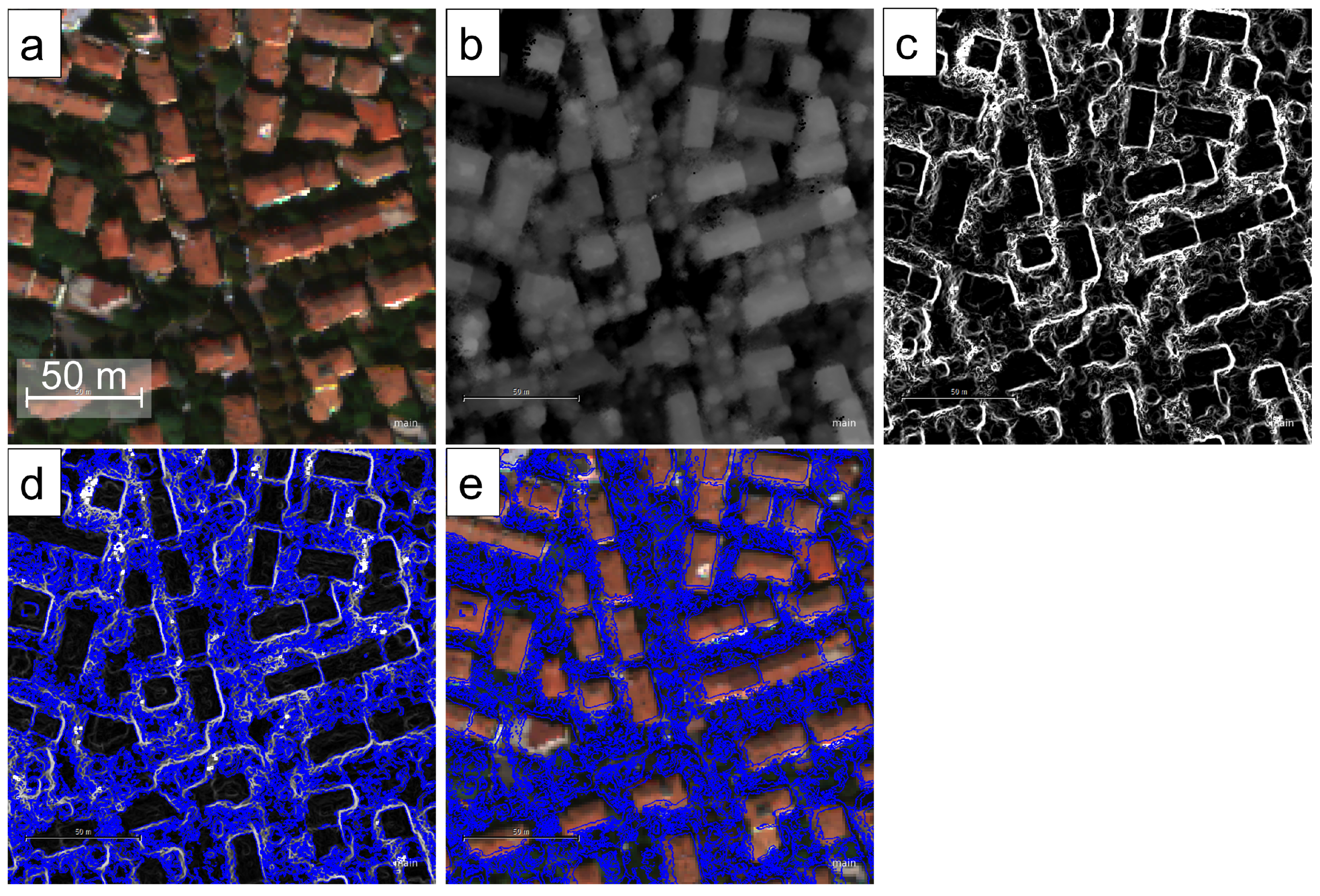
On a DSM, buildings are typically characterized by sudden changes in elevation along the perimeter, because they present very different height values compared to the surrounding environment. Moreover, a feature that allows to distinguish buildings from other landscape elements is the very steep slope at the edges [37,38]. This information was therefore obtained by applying a surface calculation algorithm to the 30 cm pixel size DSM, i.e., the Zevenbergen–Thorne method [39]. Prior to slope layer extraction, the Gauss-Blur low-pass convolution filter using the 3x3 window was applied to the DSM to reduce the effect of data noise (Figure 3b).

The “Contrast Split Segmentation” (implemented in the eCognition software) was then performed on the slope layer to generate the image objects. This algorithm was chosen due to its capability to exploit the high contrasts between the steep zones (which appear as bright pixels in Figure 3c) corresponding to building borders, and flat areas (darker pixels). Two segmentation steps were necessary: the first is applied at the pixel level to delineate steep slope objects, while the second one is applied to the first object level to separate areas with medium slope from flat ones. This segmentation approach allowed to obtain image objects very similar in shape to the buildings (Figure 3e).

The obtained objects were then classified applying sequential rules. A masking approach was performed, in order to detect and exclude from subsequent processing the objects that do not belong to buildings. Firstly, a threshold (equal to 50%) on the slope was set to identify steep objects. The NDVI (Normalized Vegetation Difference Vegetation Index) was used to exclude vegetated areas; considering WV3 imagery, the index was calculated using bands five and seven and a threshold of 0.3 was adopted. To identify the image objects actually corresponding to roofs, a rule based on the object height was applied. This feature was calculated as the difference between the DSM and the DTM derived from WV3 pairs (as described in Section 3.1). Image objects characterized by an actual height equal to or greater than two meters were assigned to the building category. A refinement rule based on the mean elevation above the sea level and the extent of the objects was introduced to avoid the erroneous inclusion of very small objects (area < 30 m²) and some very large objects located in the hilly zone (elevation > 120 m and area > 20,000 m²) that cannot be buildings. In particular, the lower limit of 30 m² can be debatable: it is thought to remove little objects that are detected as building but are actually due to unavoidable residual noise in the DSM and consequently in the slope layer. It has also the advantage of removing temporary canopies or parked truck trailers. Occasionally, it can happen that some little man-made structures are excluded (for example power cabins). However, they are not relevant for the proposed analyses, as also suggested in other studies [40].

After masking out all the objects not belonging to buildings, a multiresolution segmentation was performed, which generated a second level of objects, in order to exploit the spectral information and characterize the buildings according to their roofing material [37,41]. The segmentation algorithm was applied to the eight multispectral bands and not to the SWIR ones, due to their worse spatial resolution. The resulting new objects became the input for the supervised classification. Six informative macro-classes of roofing materials were identified, grouping the most widely used in the city:

1.

Clay tiles;

2.

Sheath;

3.

Metal sheets;

4.

Gravel;

5.

Gravel tiles;

6.

Other materials.

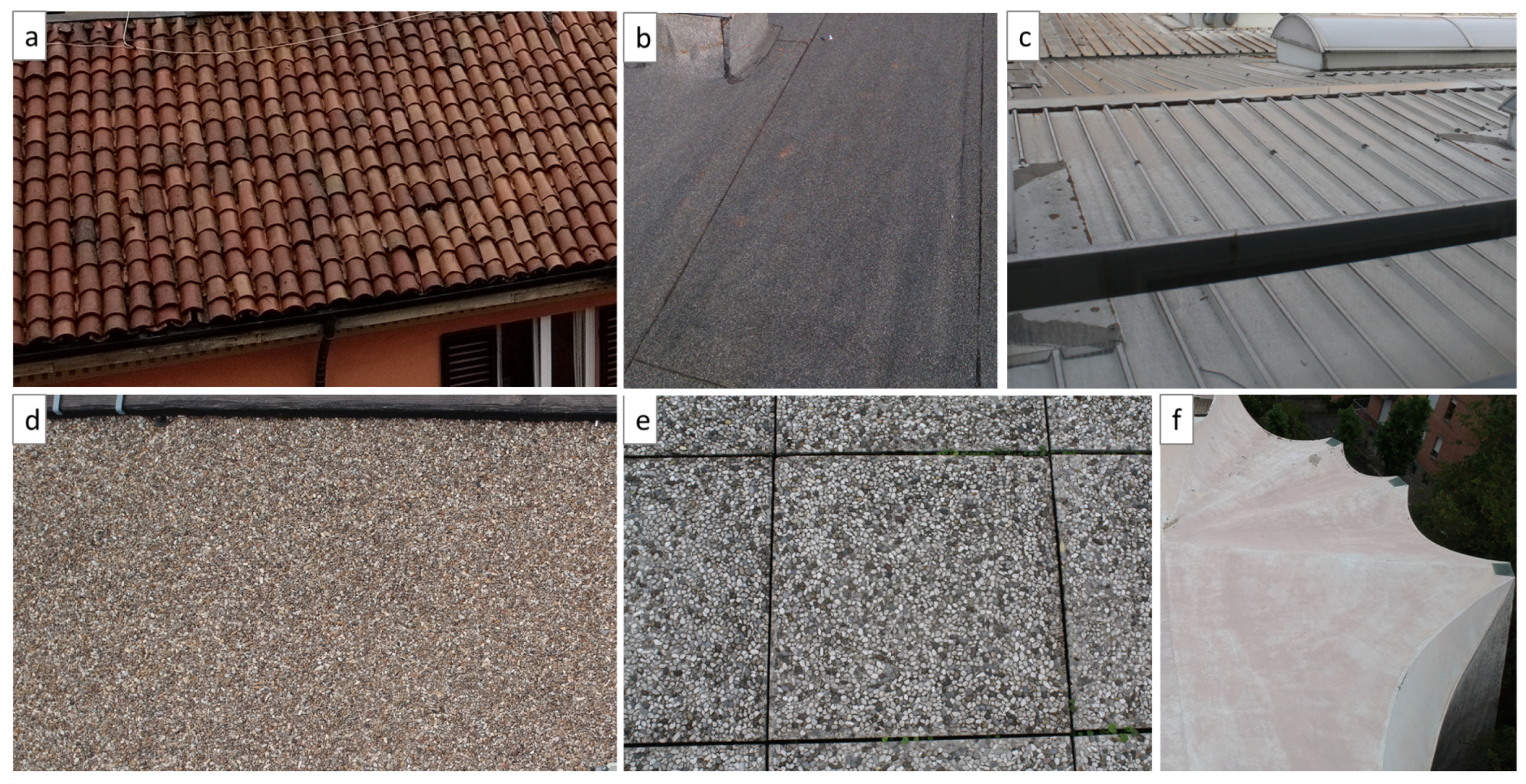
The “Clay tiles” class considers two subclasses: red- and gray-colored tiles. The great majority of buildings of the historic center has the traditional red third or half round ridge clay tiles. The “Sheath” class groups bituminous, slated and reinforced sheaths. Sheets of different alloys and with different coatings are included in the class “Metal sheets”: red, brown, green painted and uncoated metal sheets. Finally, two different classes were considered for the material gravel. “Gravel” refers to flat roof covered by a layer of loose gravel, and “Gravel tiles” refers to concrete tiles with gravel. Examples of roofing material classes are shown in Figure 4.

The training samples for each class (except ‘‘other materials”, as explained later in this section) were obtained by the field surveys (direct roof inspections and UAV flights) described in Section 2.1. After the segmentation phase, the segments corresponding to some known roofs, with surfaces as homogeneous as possible, were picked as training. Overall, 49 buildings were selected as samples encompassing the five defined classes, for a total surface of ~24,800 m² (

Table 1. Summary of the training samples used for the supervised classification of the roofing materials.

Macro Classes	Area (m2)	No. of Buildings	No. of Objects	No. of Subclasses
Clay tiles	7764.9	16	741	2
Sheath	5964.9	9	496	2
Metal sheets	6614.4	17	910	4
Gravel	2071.9	3	249	1
Gravel tiles	2428.0	4	365	1
Total	24,844.2	49	2761	10

).

A supervised sample-based machine learning algorithm was applied. The kernel based classifier SVM [42,43] was chosen, which proved to be successful with both linear and non-linear datasets [44]. Here, the following object-features were considered and computed from training samples: mean and standard deviation for all the 16 bands, texture metrics such as homogeneity and correlation (obtained through the gray level co-occurrence matrix [45]) on Red, Red-edge, and SWIR1 bands. Indeed, wavelengths corresponding to the Red and Red-edge were considered informative for the discrimination of roofing materials, especially for clay [17]. Different kernels and parameters were tested. The optimal set was found in the non-linear radial basis function kernel using parameters C and gamma equal to 100 and 0.1 respectively (see the discussion in Section 5 for further details).

Intrinsically, the SVM classifier assigns all the objects to one of the given classes by partitioning the feature space. However, although the collected samples encompass the most common materials covering the vast majority of the buildings, it is likely that some very rare ones are not included. A membership function was considered in order to exclude from the given classes those objects presenting spectral characteristics too far from the training clusters. These objects were then assigned to the “other materials” class.

Two tests were performed at this point. In the first one all the 16 WV3 bands were included in the feature space for the classification, whilst in the second one only the eight bands belonging to the multispectral sensor were used. The rationale behind this choice is to evaluate the contribution of the SWIR bands that, on the one hand, provide meaningful spectral features for material discrimination, but, on the other hand, come at a significantly lower resolution (3.4 m instead of 1.2 m).

3.4. Accuracy Assessment

The accuracy assessment is divided in two parts. The first one regards the building identification and it is performed over the whole area, while the second concerns the roofing material classification and it is limited to some check sites (as detailed below).

The first assessment was carried out in GIS environment by comparing the results obtained from the methodology previously described, with the official cartography. To avoid possible unwanted errors caused by the reference vector data, a series of checks on the building geometries and topological correctness of the reference data were performed. Furthermore, the elements not significant for the comparison were removed, i.e., canopies, shacks, cabins, walls, porticoes, kiosks, greenhouses and all the elements less than 2 m high. These elements, indeed, include structures that are temporary, very small or do not fit the definition of building.

All mapping elements were dissolved into a single geometry then separated again obtaining single polygons for each group of adjacent buildings. The output was then filtered by removing also the elements with particularly small area, less than 30 square meters. Finally, a clipping polygon was identified as the intersection between the footprint of WV3 imagery and the Municipality area. Only the area inside this polygon was considered for the accuracy analysis.

Finally, both the segments identified as buildings and the reference vector map were exported into Boolean rasters (0–1) with 0 equal to “no-building” and 1 equal to “building”, and aligned with the same grid spacing of 0.3 m.

The following step is the assessment of the material classification. A confusion matrix was computed by comparing the results of the classification with a validation dataset, made of 100 buildings, covering a total surface of more than 30,000 m². Although random sampling was not possible, the ground truth dataset was gathered from field surveys. In a GIS environment, indeed, after a proper georeferencing of the data, a new field was created in the attribute table of the technical cartography (TC); it contains the description of the roofing material, obtained by the interpretation of the close-range photographs and direct inspections.

The validation was performed considering the fact that even the most homogeneous roofs can have other materials or elements on their surface, such as rooftop HVAC (Heating, Ventilation, and Air Conditioning) units or chimneys. Moreover, trying to overcome oversegmentation problems and to realize a one-to-one object comparison, super-object level was created: all smaller objects included inside a building (as defined in the TC) were merged into a single super-object. To every super-object roof, a single class was assigned with a majority filter, i.e., the class covering the majority of its surface.

To quantitatively assess the quality of the classifications, the classic remote sensing indicators were computed from the confusion matrices, i.e., overall accuracy, producer and user accuracies and K-coefficient, as defined by Campbell [46].

4. Results

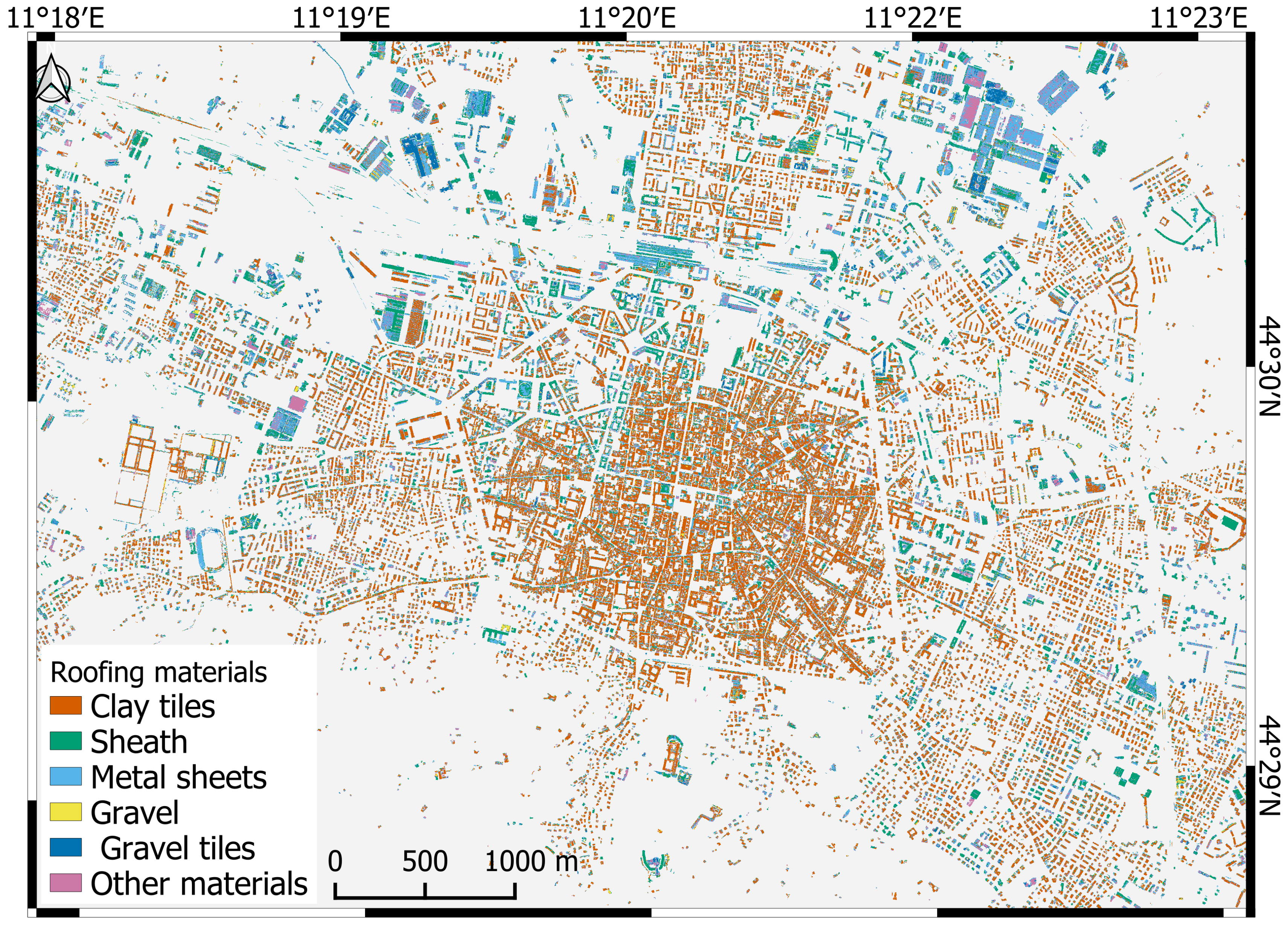
Figure 5 shows the roofing materials map obtained (with the procedure described above) using all the 16 multispectral and SWIR bands. In addition, in Figure 6 the effects of majority filter on the classification are presented. Comparing the two products, it is clear that considering every building as a single object and assigning a single material to it reduces remarkably the classification noise due to HVAC elements and smaller components on the rooftop.

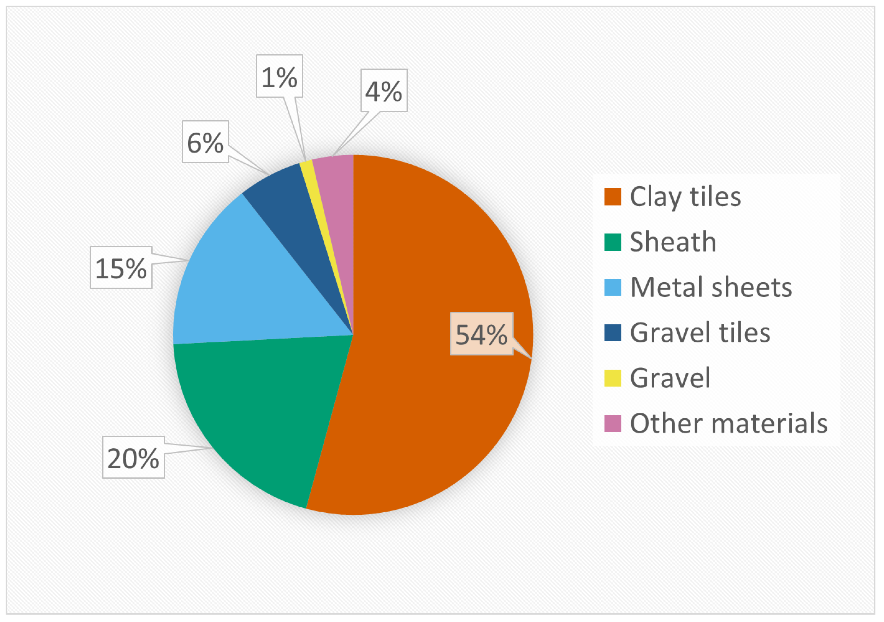
From the final classification map (Figure 6) some statistics about the occurrence of the different materials can be obtained (Figure 7). It is confirmed that the clay tile is the most used material, covering more than half (54%) of buildings in the study area. The other frequent materials are sheath (20%), followed by metals sheets used in the 15% of cases. The remaining roofs are covered by gravel tiles (6%), gravel (1%); finally, the 4% does not fall in any of the considered classes and is labeled as “other materials”.

As described in the methodology, the accuracy assessment was performed in two steps. First, the quality of the building detection was assessed over the entire area, then the performance of the material classification was checked against the collected check sites. The accuracy of the building identification procedure is summarized by the confusion matrix in

Table 2. Confusion matrix compares areas classified as buildings by the proposed procedure with the reference given by the TC of Bologna. The matrix elements are expressed in km², while the derived accuracy indicators are expressed as percentage.

		Reference
		Building	No Building
Classification	Building	9.803	2.223
	No building	2.633	79.720
	Producer accuracy	78.8%	97.3%
	User accuracy	81.5%	96.8%
	Overall accuracy	94.9%
	K coefficient	77.2%

. The detection reached an overall accuracy of 94.9%. The procedure was able to correctly identify 9.8 km² of buildings and only 2.6 out of 12.4 km² were not recognized, returning an omission error of 21.2%. In addition, a lower commission error (18.5%) was found: only 2.2 km² of the no-building area (total of 82 km²) was misclassified as buildings.

Second, the accuracy of the roofing materials map was assessed. The validation of SVM classification based on all the 16 WV3 bands was performed by computing the confusion matrix shown in

Table 3. Confusion matrix (expressed in m²) and accuracy metrics (expressed as percentage) for the classification of roofing materials obtained by considering both the multispectral and the SWIR bands.

		Reference
		Clay	Sheath	Metal	Gravel Tiles	Gravel	Other	Sum
Classification	Clay tiles	5505.4	127	369.5	0	0	0	6001.7
	Sheath	254.3	6047	215.5	0	0	0	6516.4
	Metal sheets	387.6	647	8384.9	19.4	0	0	9438.8
	Gravel tiles	0	1	51.2	4958.2	0	0	5010.7
	Gravel	0	410	0	4.9	1305.2	0	1720.3
	Other materials	8.9	0	241.6	0	0	2353.4	2603.9
	Sum	6156.3	7231.7	9262.6	4982.5	1305.2	2353.4
	Producer accuracy	89.4%	83.6%	90.5%	99.5%	100.0%	100.0%
	User accuracy	91.7%	92.8%	88.8%	99.0%	75.9%	90.4%
	Overall Accuracy	91.3%
	K coefficient	88.9%

. An overall accuracy of 91.3% was achieved (K-coefficient 88.9%).

On the other hand, the overall accuracy obtained by training the SVM only on the 8 multispectral bands and on the texture of the red and Red-Edge bands (

Table 4. Confusion matrix (expressed in m²) and accuracy metrics (expressed as percentage) for the classification of roofing materials obtained by considering only the eight multispectral bands.

		Reference
		Clay	Sheath	Metal	Gravel Tiles	Gravel	Other	Sum
Classification	Clay tiles	5312.1	0	1.4	0	257.76	0	5571.3
	Sheath	254.3	6269.0	116.5	24.3	0	0	6664.1
	Metal sheets	0	310.3	8536.0	0	0	480.4	9326.7
	Gravel tiles	0	240.1	367.2	4958.2	0	0	5565.5
	Gravel	581.0	412.2	0	0	1047.4	0	2040.6
	Other materials	8.9	0	241.6	0	0	1873.0	2123.5
	Sum	6156.3	7231.7	9262.6	4982.5	1305.2	2353.4
	Producer accuracy	80.3%	86.7%	92.2%	86.3%	99.5%	79.6%
	User accuracy	51.3%	94.1%	91.5%	95.3%	89.1%	88.2%
	Overall Accuracy	89.5%
	K coefficient	86.7%

) failed to reach the 90% threshold (89.5%, K 86.7%).

The main difference between the 16-band and 8-band solutions can be found in the clay class, where a sharp decrease in the user accuracy is observed.

5. Discussion

The proposed methodology proved to be effective in detecting and classifying roofing materials over a large area, including very different kinds of urban textures. As for the building extraction, the obtained producer accuracy (79%) is lower compared to the results achieved by some recently proposed deep learning algorithms [47,48]; these algorithms, however, require very large datasets for the training, especially to handle the complexity of different spatial structures and distributions [49]. It is worthwhile to point out that the validation adopted here is based on the TC of the municipality, which, on the one hand, has the advantage to be a fully independent dataset, and on the other hand, it comes with its own errors and small inconsistencies with imagery data. For the analysis reported in Table 2, any manual editing on the data is avoided. Other works, achieving better results, used ground-truth data based on manual delineation of features from the images themselves [50], or data that underwent a huge manual editing [40].

In the proposed detection approach, the variations in the urban texture impact on the complexity of the rule set for the segmentation phase. For example, the historic city center, mainly flat, completely built-up with buildings close or even connected to each other, differs a lot from the residential zone in the southern part of the study area. That zone indeed is hilly and covered by woods surrounding mainly detached houses. In this context a segmentation based on the slope instead of the original DSM proved to be effective.

The burdensome requirement of a large training set limits the adoption of deep learning algorithms for roofing materials classification, because in many practical cases ground-truth datasets are relatively small and they can be exploited more efficiently with SVM [51]. Here, the achieved accuracies (overall 91%, user and producer reported in Table 3) are comparable (or outperform in some cases) with the reported experiments using similar imagery and OBIA approach [12,13,14], and also with few works exploiting convolutional neural networks but with a more limited number of material classes [9,23].

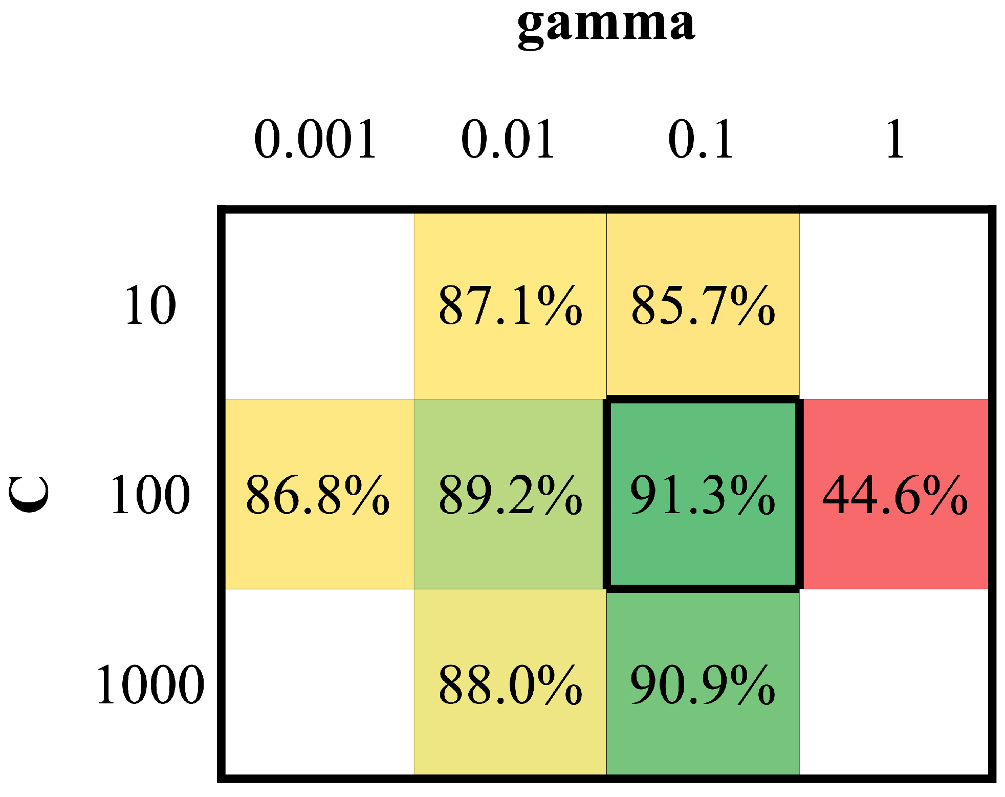
A critical step in the described approach is the parameterization of the SVM algorithm. The choice of the set of parameters has a significant impact on the final accuracy. Indeed, different parameters were tested for the optimization of the solution (using 16 bands), as summarized in Figure 8. The adopted set is the one resulting in the highest accuracy.

The inclusion of the SWIR bands improved the quality of the final solution, especially for clay. This might be due to the fact that some distinctive spectral features of clay minerals appear in the SWIR region. Overall, the rate of the improvement is a trade-off between the additional spectral information content and the lower spatial resolution, which might smooth spectral signature differences. However, using the texture metrics, the lower resolution of the SWIR band may have the positive effect of reducing the noise due to HVAC units or chimneys on the rooftops.

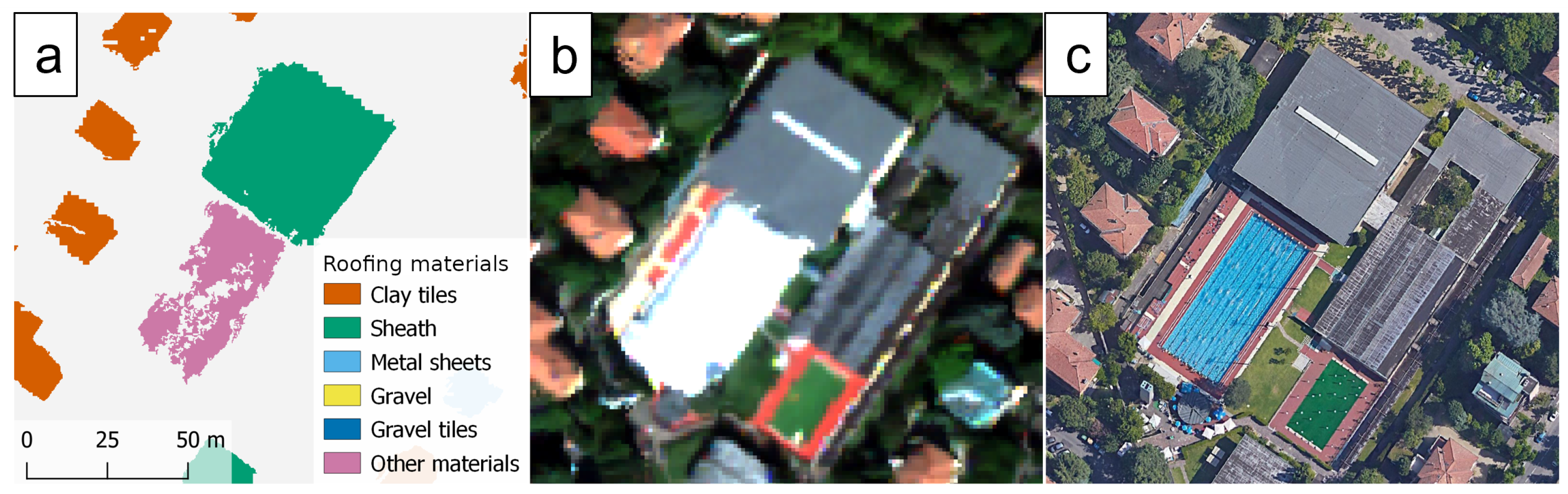
As for the considered classes, the classification included the most used roofing solutions, but took into account also the possible occurrence of rare materials. One example of such a situation is depicted in Figure 9, where the temporary cover of a swimming pool is correctly assigned to the other material class. The shape of the detected object appears irregular, probably as a consequence of the rounded and convex surface of the dome inflatable structure, which is poorly resolved by the photogrammetric DSM.

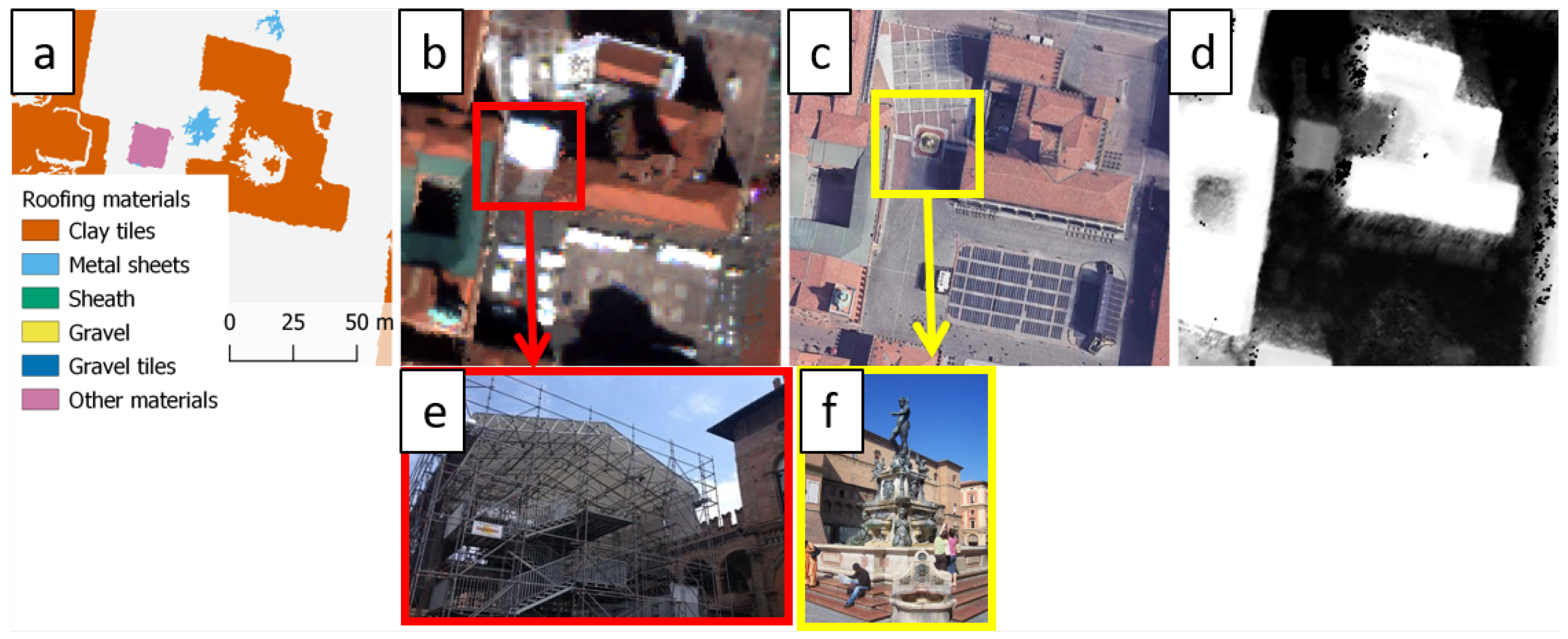
Another example of other material is the tensile structure realized for the restoration of the Neptune statue in the city center in 2017, as shown in Figure 10. It can be noted that close to the upper right corner of the “other materials” there is a false detection of a metal roof. Probably, this misclassification is due to an artifact of the DSM occurring in a shadowed area of the original image.

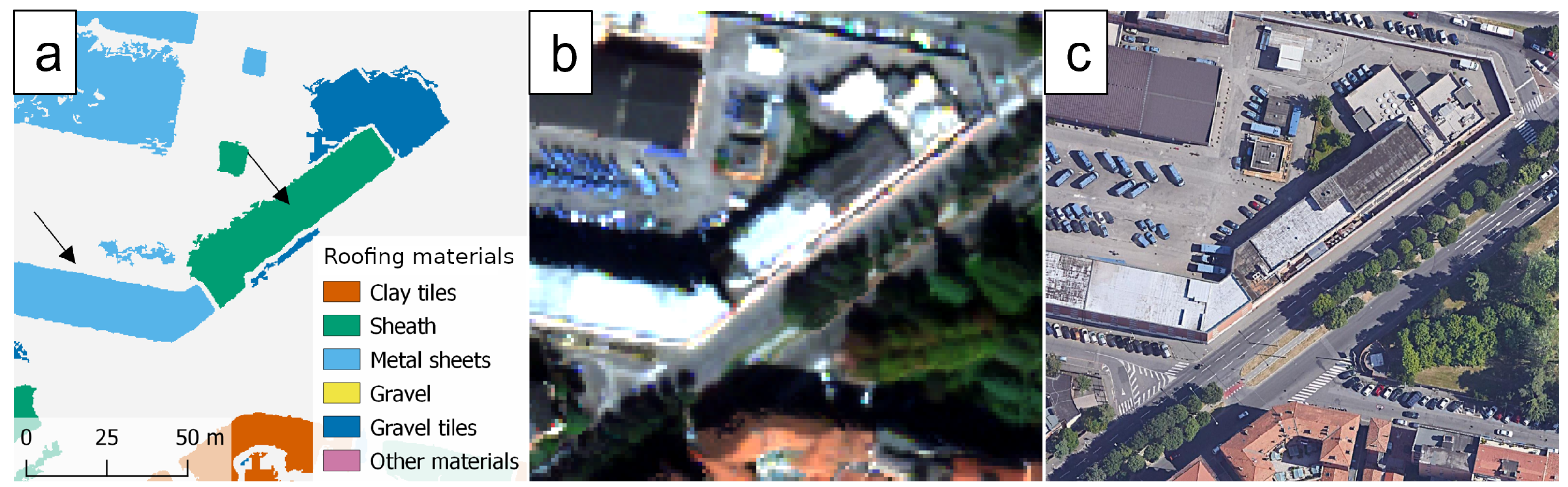
Investigating the commission errors outlined by the confusion matrix, it can be pointed out that some errors are related to paintings and coatings of sheath membranes. For example, the two buildings in Figure 11 are classified as metal sheets and bituminous sheath, respectively, when actually they are both covered by sheaths. One of them (indicated by the left arrow in Figure 11a) has an aluminum paint over the whole surface, while the other (right arrow) is only partially painted. When dominant, this aluminum paint led to a misclassification as a metal roof. Regarding the paintings, also aging effects may have consequences on the spectral signature of the material (as highlighted also by [53,54]) and in turn on the assignment of the objects.

The class with the lower user accuracy is the gravel (Table 3). This fact may be related to two possible causes. First, gravel can show large variations in the spectral signature depending on the lithology of the originating rocks. The second aspect is the unbalance of the training dataset (see Table 1, where gravels appears to be the minority class). Sampling unbalance, indeed, typically does not affect the overall accuracy, but has a considerable impact on the accuracy of the minority class [55]. For relatively rare classes, however, it is difficult to obtain a numerous set of samples from surveys, especially given the strict regulations on drone flights in urban areas. Among the mitigation strategies proposed in the literature [55], the under-sampling, over-sampling or the adjustment of the cost function of the SVM may be suitable for these situations and may deserve further investigations.

Another delicate point in the proposed classification approach is the application of the majority filter. This step is necessary for the validation phase in order to establish a correspondence between the ground truth objects derived by the TC and the objects coming from the image segmentation. The oversegmentation problem, indeed, is widespread all over the processed area. Only considering the 100 validation buildings, the median number of segments belonging to one super-object is 35 (with an interquartile range of 50). In half of the super-objects, more than the 70% of the area is covered by the dominant class, while it covers less then 50% of the area only in one quarter of them. This is caused by the occurrence of many small segments of different classes inside almost every building.

As a consequence, the majority filter has a certain impact on the final map. On the one hand, it strongly improves the results by removing some noise due to the presence of chimneys, HVAC units, and skylights, which produce small objects of different classes. It also removes errors occurring at the edges of the roofs, where some segments sometimes include pixels from the facades or the ground. On the other hand, some disadvantages can arise when the roofs of large buildings are covered by different materials over different wings, but they belong to a single super-object. 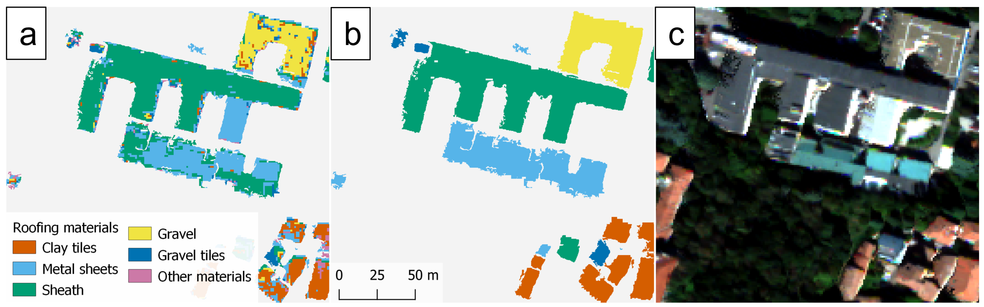One example of these positive and negative consequences can be seen in Figure 12, where the gravel roof (yellow) appears cleaned from spurious objects after the majority filter, while one correctly classified metal wing (cyan) of the central building is merged with the dominant sheath cover (green).

In the perspective of applying the methodology to the management and urban planning of wide metropolitan areas, the adoption of the majority filter produces more homogeneous maps that may fit better the level of detail required by stakeholders.

The obtained classification considers the major categories of roofing materials. Additional experiments and analyses are necessary to verify the capability of multispectral stereo-images to expand the number of classes that can be discriminated. Other aspects to be addressed in future works are a finer analysis on the impact of the segmentation parameters on the SVM results, and how to handle the majority filter without a TC. Regarding this last point, possible alternative sources of vector data may be OpenStreetMap [56] or other crowd mapping initiatives [10].

6. Conclusions

A methodology was presented for the detection of buildings and the classification of the roofing materials over an area of approximately 100 km² and a wide variety of urban textures. It relies only on very high-resolution multispectral images with stereo capabilities acquired by a satellite platform. This makes the procedure highly replicable virtually in any part of the world, since it does not require expensive datasets acquired on the field or by dedicated aerial surveys (such as LiDAR data). The achieved overall accuracy—approximately 91% in roofing classification—is comparable with most of the published works on these topics but applies on a wider area. Most of the observed errors are related to artifacts or defects in the photogrammetric digital surface model, or to the presence of certain coatings that may hide the distinctive spectral features of the roofing materials. Despite these residual errors, the proposed approach can be used to conduct a census of the major roofing materials in a city.