
On the 3D Reconstruction of Coastal Structures by Unmanned Aerial Systems with Onboard Global Navigation Satellite System and Real-Time Kinematics and Terrestrial Laser Scanning


Abstract
:
1. Introduction
2. Methods
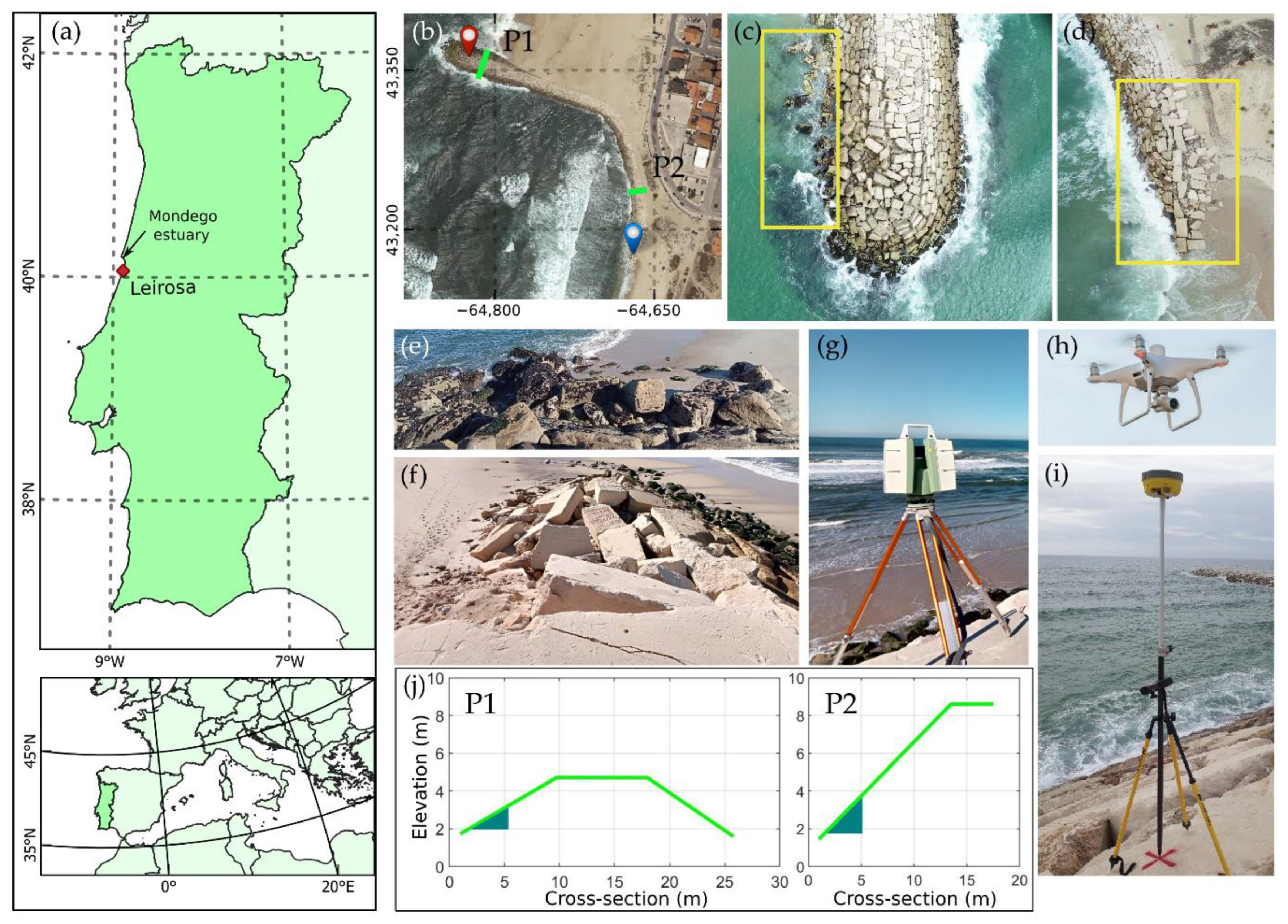
2.1. Study Site
2.2. Unmanned Aerial System Data Acquisition and Processing
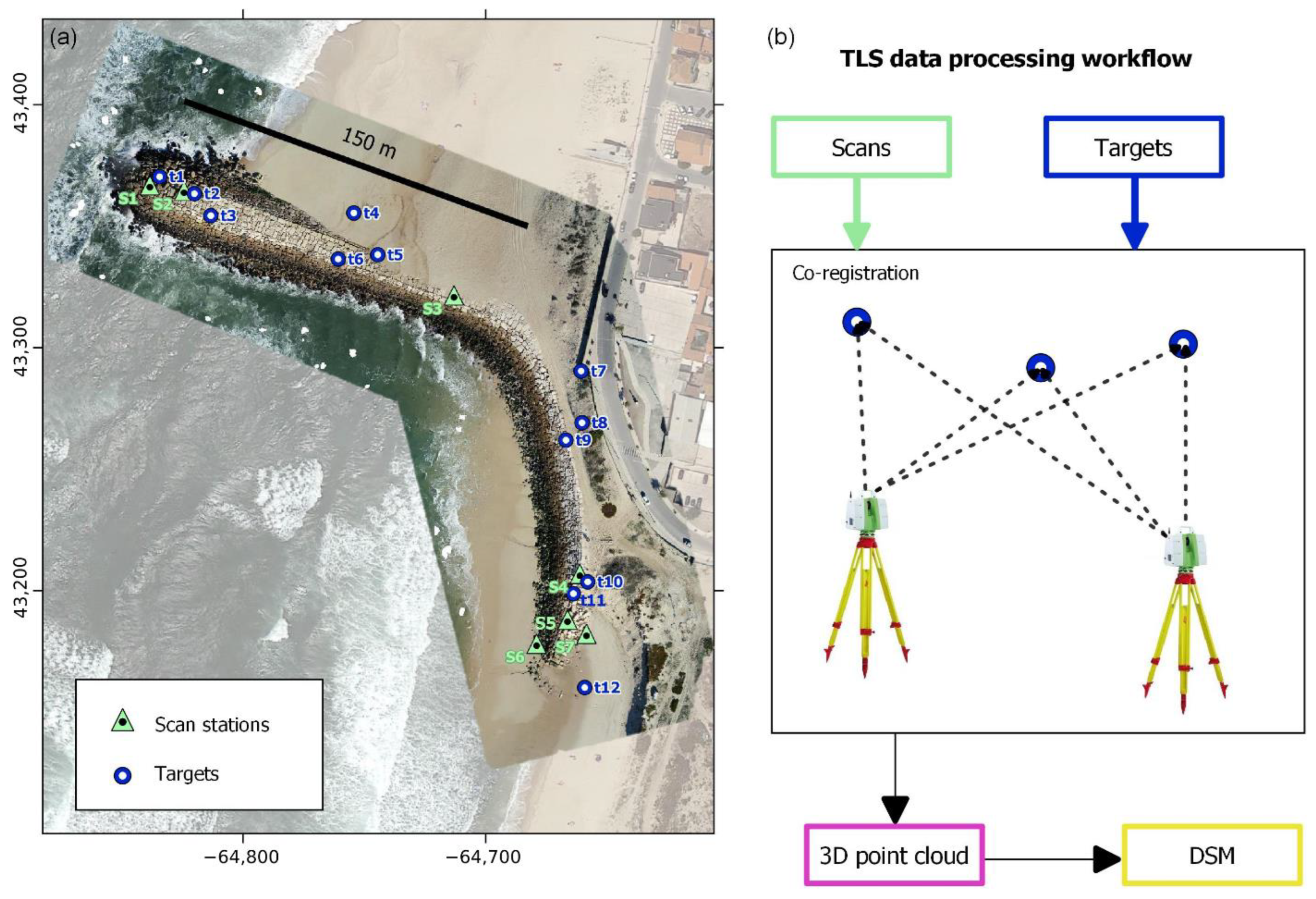
2.3. Terrestrial Laser Scanning Data Acquisition and Processing
2.4. Three-Dimensional Point Clouds and Digital Surface Model
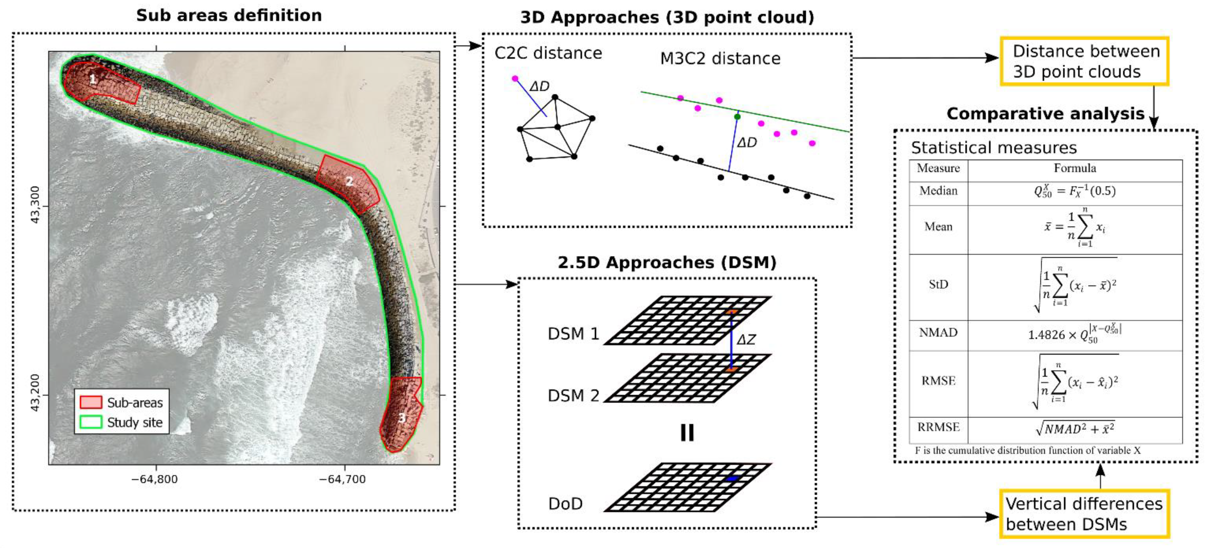
2.5. Comparative Analysis and Statistical Measures
3. Results
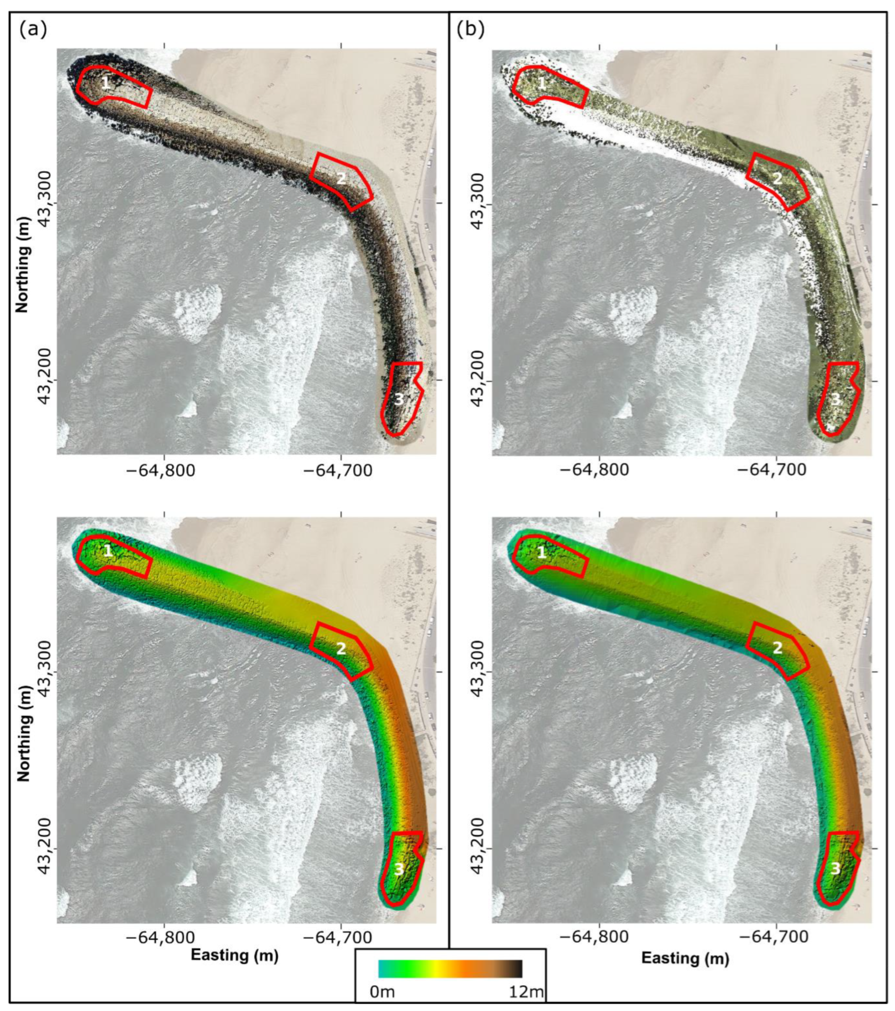
3.1. 3D Point Clouds and Digital Surface Model
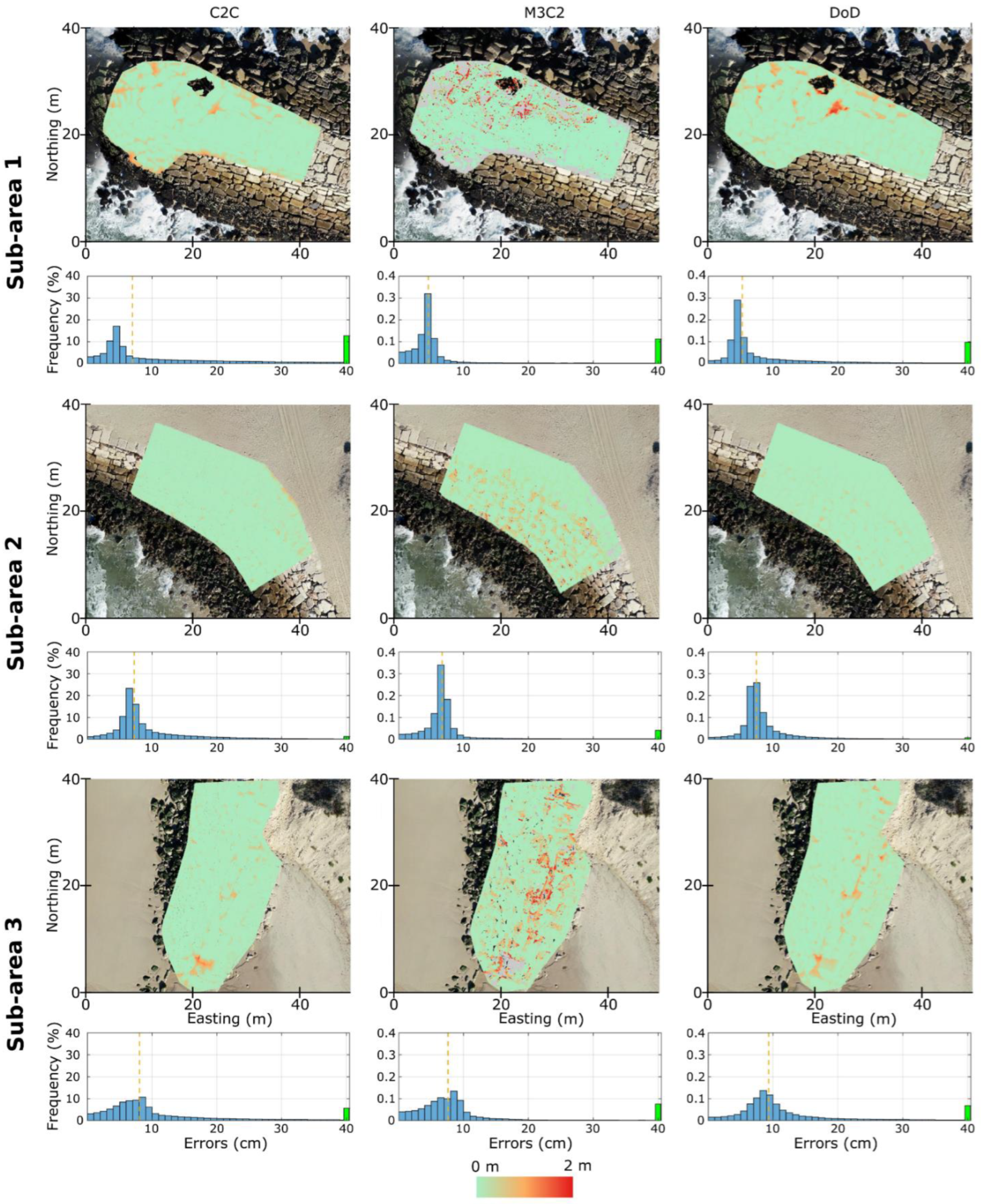
3.2. Comparative Analysis and Statistical Measures of 3D Point Clouds and DSM
4. Discussion
5. Conclusions
Author Contributions
Funding
Institutional Review Board Statement
Informed Consent Statement
Data Availability Statement
Acknowledgments
Conflicts of Interest
References
- CIRIA; CUR; CETMEF. The Rock Manual. The Use of Rock in Hydraulic Engineering, 2nd ed.; C683; CIRIA: London, UK, 2007; ISBN 9780860176831. [Google Scholar]
- U.S. Army Corps of Engineers. Coastal Engineering Manual (EM 1110-2-1100); U.S. Army Corps of Engineers: Washington, DC, USA, 2002. [Google Scholar]
- Kamphuis, J.W. Introduction to Coastal Engineering and Management; World Scientific: Singapore, 2000; ISBN 981-02-3830-4. [Google Scholar]
- Oliveira, J.N.C.; Oliveira, F.S.B.F.; Neves, M.G.; Clavero, M.; Trigo-Teixeira, A.A. Modeling wave overtopping on a seawall with XBeach, IH2VOF, and mase formulas. Water 2020, 12, 2526. [Google Scholar] [CrossRef]
- Reis, M.T.; Neves, M.G.; Lopes, M.R.; Hu, K.; Silva, L.G. Rehabilitation of sines west breakwater: Wave overtopping study. Proc. Inst. Civ. Eng. Marit. Eng. 2011, 164, 15–32. [Google Scholar] [CrossRef] [Green Version]
- Santos, C.J.; Andriolo, U.; Ferreira, J.C. Shoreline response to a sandy nourishment in a wave-dominated coast using video monitoring. Water 2020, 12, 1632. [Google Scholar] [CrossRef]
- Allen, R.T. Concrete in Coastal Structures; Thomas Telford: London, UK, 1998. [Google Scholar]
- Isobe, M. Impact of global warming on coastal structures in shallow water. Ocean Eng. 2013, 71, 51–57. [Google Scholar] [CrossRef]
- Dos Reis, M.T.L.G.V.; Poseiro, P.G.G.; Fortes, C.J.E.M.; Conde, J.M.P.; Didier, E.L.; Sabino, A.M.G.; Grueau, M.A.S.R. Risk management in maritime structures. In Proceedings of the Eighth International Conference on Management Science and Engineering Management: Focused on Computing and Engineering Management, Lisbon, Portugal, 25–27 July 2014; Volume 281, pp. 1179–1190. [Google Scholar]
- Santos, J.A.; Neves, M.D.G.; Silva, L.G. Rubble-mound breakwater inspection in Portugal. In Proceedings of the Coastal Structures 2003, Portland, OR, USA, 26–30 August 2003; pp. 249–261. [Google Scholar]
- Silvestre, C.; Oliveira, P.; Pascoal, A.; Sebastião, L.; Alves, J.; Santos, J.A.; Silva, L.G.; Neves, M.D.G. Inspection and Diagnosis of Sines’ West Breakwater. Coast. Eng. 2005, 4, 3555–3567. [Google Scholar]
- Lemos, R.; Capitão, R.; Fortes, C.; Henriques, M.; Silva, L.G.; Martins, T. A methodology for the evaluation of evolution and risk of breakwaters. Application to Portimão harbor and of Faro-Olhão inlet. J. Integr. Coast. Zone Manag. 2020, 20, 103–119. [Google Scholar] [CrossRef]
- Puente, I.; Sande, J.; González-Jorge, H.; Peña-González, E.; Maciñeira, E.; Martínez-Sánchez, J.; Arias, P. Novel image analysis approach to the terrestrial LiDAR monitoring of damage in rubble mound breakwaters. Ocean Eng. 2014, 91, 273–280. [Google Scholar] [CrossRef]
- Tmušić, G.; Manfreda, S.; Aasen, H.; James, M.R.; Gonçalves, G.; Ben-Dor, E.; Brook, A.; Polinova, M.; Arranz, J.J.; Mészáros, J.; et al. Current practices in UAS-based environmental monitoring. Remote Sens. 2020, 12, 1001. [Google Scholar] [CrossRef] [Green Version]
- Manfreda, S.; Mccabe, M.F.; Miller, P.E.; Lucas, R.; Pajuelo, V.M.; Mallinis, G.; Ben Dor, E.; Helman, D.; Estes, L.; Ciraolo, G.; et al. Use of Unmanned Aerial Systems for Environmental Monitoring. Remote Sens. 2018, 10, 641. [Google Scholar] [CrossRef] [Green Version]
- Andriolo, U.; Gonçalves, G.; Sobral, P.; Fontán-Bouzas, Á.; Bessa, F. Beach-dune morphodynamics and marine macro-litter abundance: An integrated approach with Unmanned Aerial System. Sci. Total Environ. 2020, 749, 141474. [Google Scholar] [CrossRef]
- Duo, E.; Chris Trembanis, A.; Dohner, S.; Grottoli, E.; Ciavola, P. Local-scale post-event assessments with GPS and UAV-based quick-response surveys: A pilot case from the Emilia-Romagna (Italy) coast. Nat. Hazards Earth Syst. Sci. 2018, 18, 2969–2989. [Google Scholar] [CrossRef] [Green Version]
- Duo, E.; Fabbri, S.; Grottoli, E.; Ciavola, P. Uncertainty of drone-derived dems and significance of detected morphodynamics in artificially scraped dunes. Remote Sens. 2021, 13, 1823. [Google Scholar] [CrossRef]
- Fairley, I.; Horrillo-Caraballo, J.; Masters, I.; Karunarathna, H.; Reeve, D.E. Spatial variation in coastal dune evolution in a high tidal range environment. Remote Sens. 2020, 12, 3689. [Google Scholar] [CrossRef]
- Bastos, A.P.; Lira, C.P.; Calvão, J.; Catalão, J.; Andrade, C.; Pereira, A.J.; Taborda, R.; Rato, D.; Pinho, P.; Correia, O. UAV Derived Information Applied to the Study of Slow-changing Morphology in Dune Systems. J. Coast. Res. 2018, 85, 226–230. [Google Scholar] [CrossRef]
- Taddia, Y.; Corbau, C.; Zambello, E.; Pellegrinelli, A. UAVs for structure-from-motion coastal monitoring: A case study to assess the evolution of embryo dunes over a two-year time frame in the po river delta, Italy. Sensors 2019, 19, 1717. [Google Scholar] [CrossRef] [PubMed] [Green Version]
- Luppichini, M.; Bini, M.; Paterni, M.; Berton, A.; Merlino, S. A new beach topography-based method for shoreline identification. Water 2020, 12, 3110. [Google Scholar] [CrossRef]
- Gonçalves, G.; Santos, S.; Duarte, D.; Gomes, J. Monitoring Local Shoreline Changes by Integrating UASs, Airborne LiDAR, Historical Images and Orthophotos. In Proceedings of the 5th International Conference on Geographical Information Systems Theory, Applications and Management, Crete, Greece, 3–5 May 2019; Scitepress—Science and Technology Publications: Setúbal, Portugal; pp. 126–134. [Google Scholar]
- Jaud, M.; Letortu, P.; Théry, C.; Grandjean, P.; Costa, S.; Maquaire, O.; Davidson, R.; Le Dantec, N. UAV survey of a coastal cliff face—Selection of the best imaging angle. Meas. J. Int. Meas. Confed. 2019, 139, 10–20. [Google Scholar] [CrossRef] [Green Version]
- Gómez-Gutiérrez, Á.; Gonçalves, G.R. Surveying coastal cliffs using two UAV platforms (multi-rotor and fixed- wing) and three different approaches for the estimation of volumetric changes. Int. J. Remote Sens. 2020, 41, 8143–8175. [Google Scholar] [CrossRef]
- Gonçalves, G.; Gonçalves, D.; Gómez-gutiérrez, Á.; Andriolo, U.; Pérez-alvárez, J.A. 3d reconstruction of coastal cliffs from fixed-wing and multi-rotor uas: Impact of sfm-mvs processing parameters, image redundancy and acquisition geometry. Remote Sens. 2021, 13, 1222. [Google Scholar] [CrossRef]
- Andriolo, U.; Gonçalves, G.; Sobral, P.; Bessa, F. Spatial and size distribution of macro-litter on coastal dunes from drone images: A case study on the Atlantic coast. Mar. Pollut. Bull. 2021, 169, 112490. [Google Scholar] [CrossRef] [PubMed]
- Duarte, D.; Andriolo, U.; Gonçalves, G. Addressing the Class Imbalance Problem in the Automatic Image Classification of Coastal Litter From Orthophotos Derived From Uas Imagery. ISPRS Ann. Photogramm. Remote Sens. Spat. Inf. Sci. 2020, 3, 439–445. [Google Scholar] [CrossRef]
- Andriolo, U.; Gonçalves, G.; Rangel-Buitrago, N.; Paterni, M.; Bessa, F.; Gonçalves, L.M.S.; Sobral, P.; Bini, M.; Duarte, D.; Fontán-Bouzas, Á.; et al. Drones for litter mapping: An inter-operator concordance test in marking beached items on aerial images. Mar. Pollut. Bull. 2021, 169, 112542. [Google Scholar] [CrossRef] [PubMed]
- Gonçalves, G.; Andriolo, U.; Pinto, L.; Bessa, F. Mapping marine litter using UAS on a beach-dune system: A multidisciplinary approach. Sci. Total Environ. 2020, 706, 135742. [Google Scholar] [CrossRef]
- Gonçalves, G.; Andriolo, U.; Gonçalves, L.; Sobral, P.; Bessa, F. Quantifying Marine Macro Litter Abundance on a Sandy Beach Using Unmanned Aerial Systems and Object-Oriented Machine Learning Methods. Remote Sens. 2020, 12, 2599. [Google Scholar] [CrossRef]
- Taddia, Y.; Corbau, C.; Buoninsegni, J.; Simeoni, U.; Pellegrinelli, A. UAV Approach for Detecting Plastic Marine Debris on the Beach: A Case Study in the Po River Delta (Italy). Drones 2021, 5, 140. [Google Scholar] [CrossRef]
- Andriolo, U.; Garcia-garin, O.; Vighi, M.; Borrell, A.; Gonçalves, G. Beached and Floating Litter Surveys by Unmanned Aerial Vehicles: Operational Analogies and Differences. Remote Sens. 2022, 14, 1336. [Google Scholar] [CrossRef]
- Gonçalves, G.; Andriolo, U. Operational use of multispectral images for macro-litter mapping and categorization by Unmanned Aerial Vehicle. Mar. Pollut. Bull. 2022, 176, 113431. [Google Scholar] [CrossRef] [PubMed]
- Smith, M.W.; Carrivick, J.L.; Quincey, D.J. Structure from motion photogrammetry in physical geography. Prog. Phys. Geogr. 2015, 40, 247–275. [Google Scholar] [CrossRef] [Green Version]
- Taddia, Y.; González-García, L.; Zambello, E.; Pellegrinelli, A. Quality Assessment of Photogrammetric Models for Façade and Building Reconstruction Using DJI Phantom 4 RTK. Remote Sens. 2020, 12, 3144. [Google Scholar] [CrossRef]
- Štroner, M.; Urban, R.; Seidl, J.; Reindl, T.; Brouček, J. Photogrammetry Using UAV-Mounted GNSS RTK: Georeferencing Strategies without GCPs. Remote Sens. 2021, 13, 1336. [Google Scholar] [CrossRef]
- Bosma, C.; Civiel, S.; Verhagen, H.J. Void porosity measurements in coastal structures. In Coastal Engineering 2002; World Scientific Publishing Company: Singapore, 2002; pp. 1411–1423. [Google Scholar] [CrossRef] [Green Version]
- Henriques, M.J.; Fonseca, A.; Roque, D.; Lima, J.N.; Marnoto, J. Assessing the Quality of an UAV-based Orthomosaic and Surface Model of a Breakwater. 2014, pp. 1–16. Available online: https://mycoordinates.org/assessing-the-quality-of-an-uav-based-orthomosaic-and-surface-model-of-a-breakwater/ (accessed on 14 February 2022).
- González-Jorge, H.; Puente, I.; Roca, D.; Martínez-Sánchez, J.; Conde, B.; Arias, P. UAV Photogrammetry Application to the Monitoring of Rubble Mound Breakwaters. J. Perform. Constr. Facil. 2016, 30, 04014194. [Google Scholar] [CrossRef]
- King, S.; Leon, J.; Mulcahy, M.; Jackson, L.A.; Corbett, B. Condition survey of coastal structures using UAV and photogrammetry. In Proceedings of the Australasian Coasts & Ports conference, Cairns, Australia, 21–23 June 2017; pp. 704–710. [Google Scholar]
- Mendes, D.; Pais-Barbosa, J.; Baptista, P.; Silva, P.A.; Bernardes, C.; Pinto, C. Beach Response to a Shoreface Nourishment (Aveiro, Portugal). J. Mar. Sci. Eng. 2021, 9, 1112. [Google Scholar] [CrossRef]
- Andriolo, U.; Mendes, D.; Taborda, R. Breaking wave height estimation from timex images: Two methods for coastal video monitoring systems. Remote Sens. 2020, 12, 204. [Google Scholar] [CrossRef] [Green Version]
- Fernández-Fernández, S.; Ferreira, C.C.; Silva, P.A.; Baptista, P.; Romão, S.; Fontán-Bouzas, Á.; Abreu, T.; Bertin, X. Assessment of dredging scenarios for a tidal inlet in a high-energy coast. J. Mar. Sci. Eng. 2019, 7, 395. [Google Scholar] [CrossRef] [Green Version]
- Ferreira, C.; Silva, P.A.; Fernández-Fernández, S.; Baptista, P.; Abreu, T.; Romão, S.; Fontán-Bouzas, Á.; Bertin, X.; Garrido, C. Wave Climate Definition on Modeling Morphological Changes in Figueira da Foz Coastal System (W Portugal). J. Coast. Res. 2018, 85, 1256–1260. [Google Scholar] [CrossRef]
- Ponte Lira, C.; Silva, A.N.; Taborda, R.; De Andrade, C.F. Coastline evolution of Portuguese low-lying sandy coast in the last 50 years: An integrated approach. Earth Syst. Sci. Data 2016, 8, 265–278. [Google Scholar] [CrossRef] [Green Version]
- Taddia, Y.; Stecchi, F.; Pellegrinelli, A. Coastal Mapping Using DJI Phantom 4 RTK in Post-Processing Kinematic Mode. Drones 2020, 4, 9. [Google Scholar] [CrossRef] [Green Version]
- Rangel, J.M.G.; Gonçalves, G.; Pérez, J.A. The impact of number and spatial distribution of GCPs on the positional accuracy of geospatial products derived from low-cost UASs. Int. J. Remote Sens. 2018, 39, 7154–7171. [Google Scholar] [CrossRef]
- Lague, D.; Brodu, N.; Leroux, J. Accurate 3D comparison of complex topography with terrestrial laser scanner: Application to the Rangitikei canyon (N-Z). ISPRS J. Photogramm. Remote Sens. 2013, 82, 10–26. [Google Scholar] [CrossRef] [Green Version]
- Höhle, J.; Höhle, M. Accuracy assessment of digital elevation models by means of robust statistical methods. ISPRS J. Photogramm. Remote Sens. 2009, 64, 398–406. [Google Scholar] [CrossRef] [Green Version]
- Gonçalves, G.R.; Pérez, J.A.; Duarte, J. Accuracy and effectiveness of low cost UASs and open source photogrammetric software for foredunes mapping. Int. J. Remote Sens. 2018, 39, 5059–5077. [Google Scholar] [CrossRef]
- Medjkane, M.; Maquaire, O.; Costa, S.; Roulland, T.; Letortu, P.; Fauchard, C.; Antoine, R.; Davidson, R. High-resolution monitoring of complex coastal morphology changes: Cross-efficiency of SfM and TLS-based survey (Vaches-Noires cliffs, Normandy, France). Landslides 2018, 15, 1097–1108. [Google Scholar] [CrossRef]
- Lin, Y.-C.; Cheng, Y.-T.; Zhou, T.; Ravi, R.; Hasheminasab, S.M.; Flatt, J.E.; Troy, C.; Habib, A. Evaluation of UAV LiDAR for mapping coastal environments. Remote Sens. 2019, 11, 2893. [Google Scholar] [CrossRef] [Green Version]
- Tu, Y.H.; Johansen, K.; Aragon, B.; Stutsel, B.M.; Angel, Y.; Camargo, O.A.L.; Al-Mashharawi, S.K.M.; Jiang, J.; Ziliani, M.G.; McCabe, M.F. Combining Nadir, Oblique, and Façade Imagery Enhances Reconstruction of Rock Formations Using Unmanned Aerial Vehicles. IEEE Trans. Geosci. Remote Sens. 2021, 59, 9987–9999. [Google Scholar] [CrossRef]
- Rossi, P.; Mancini, F.; Dubbini, M.; Mazzone, F.; Capra, A. Combining nadir and oblique uav imagery to reconstruct quarry topography: Methodology and feasibility analysis. Eur. J. Remote Sens. 2017, 50, 211–221. [Google Scholar] [CrossRef] [Green Version]
- Han, S.; Jiang, Y.; Bai, Y. Fast-PGMED: Fast and Dense Elevation Determination for Earthwork Using Drone and Deep Learning. J. Constr. Eng. Manag. 2022, 148, 04022008. [Google Scholar] [CrossRef]
- Shang, Z.; Shen, Z. Real-time 3D reconstruction on construction site using visual SLAM and UAV. Constr. Res. Congr. Constr. Inf. Technol.-Sel. Pap. Constr. Res. Congr. 2018, 2018, 305–315. [Google Scholar] [CrossRef] [Green Version]
- Valero, E.; Bosché, F.; Forster, A. Automatic segmentation of 3D point clouds of rubble masonry walls, and its application to building surveying, repair and maintenance. Autom. Constr. 2018, 96, 29–39. [Google Scholar] [CrossRef]


| Parameters | Unmanned Aerial System | Terrestrial Laser Scanner | |
|---|---|---|---|
| Whole structure (6630 m2) | Number of points | 11.3 × 10⁶ | 41.3 × 10⁶ |
| Mean surface density (points/m2) | 1.7 × 10³ | 6.2 × 10³ | |
| Data gaps (%) | 0 | 16.8 | |
| Sub-area 1 (560 m2) | Number of points | 1.0 × 10⁶ | 15.2 × 10⁶ |
| Mean surface density (points/m2) | 1.8 × 10³ | 27.2 × 10³ | |
| Data gaps (%) | 0 | 1.4 | |
| Sub-area 2 (530 m2) | Number of points | 0.9 × 10⁶ | 0.7 × 10⁶ |
| Mean surface density (points/m2) | 1.6 × 10³ | 1.3 × 10³ | |
| Data gaps (%) | 0 | 0 | |
| Sub-area 3 (600 m2) | Number of points | 1.2 × 10⁶ | 21.8 × 10⁶ |
| Mean surface density (points/m2) | 2.0 × 10³ | 36.4 × 10³ | |
| Data gaps (%) | 0 | 0.8 |
| Approach | Sub-Area | Mean (cm) | Median (cm) | Std (cm) | NMAD (cm) | RMSE (cm) | RRMSE (cm) |
|---|---|---|---|---|---|---|---|
| C2C | 1 | 17.2 | 7.0 | 21.1 | 6.4 | 27.2 | 18.4 |
| 2 | 10.0 | 7.2 | 7.9 | 2.3 | 12.7 | 10.3 | |
| 3 | 12.9 | 8.1 | 15.3 | 5.0 | 20.0 | 13.8 | |
| M3C2 | 1 | 16.8 | 4.6 | 36.0 | 1.6 | 39.8 | 16.9 |
| 2 | 10.2 | 6.7 | 16.5 | 1.3 | 19.4 | 10.3 | |
| 3 | 14.4 | 7.6 | 26.8 | 3.5 | 30.4 | 14.8 | |
| DoD | 1 | 14.9 | 5.3 | 23.8 | 2.3 | 28.1 | 15.0 |
| 2 | 9.0 | 7.4 | 6.0 | 1.5 | 10.8 | 9.1 | |
| 3 | 14.5 | 9.3 | 16.1 | 3.8 | 21.7 | 15.0 |
Publisher’s Note: MDPI stays neutral with regard to jurisdictional claims in published maps and institutional affiliations. |
© 2022 by the authors. Licensee MDPI, Basel, Switzerland. This article is an open access article distributed under the terms and conditions of the Creative Commons Attribution (CC BY) license (https://creativecommons.org/licenses/by/4.0/).
Share and Cite
Gonçalves, D.; Gonçalves, G.; Pérez-Alvávez, J.A.; Andriolo, U. On the 3D Reconstruction of Coastal Structures by Unmanned Aerial Systems with Onboard Global Navigation Satellite System and Real-Time Kinematics and Terrestrial Laser Scanning. Remote Sens. 2022, 14, 1485. https://doi.org/10.3390/rs14061485
Gonçalves D, Gonçalves G, Pérez-Alvávez JA, Andriolo U. On the 3D Reconstruction of Coastal Structures by Unmanned Aerial Systems with Onboard Global Navigation Satellite System and Real-Time Kinematics and Terrestrial Laser Scanning. Remote Sensing. 2022; 14(6):1485. https://doi.org/10.3390/rs14061485
Chicago/Turabian StyleGonçalves, Diogo, Gil Gonçalves, Juan Antonio Pérez-Alvávez, and Umberto Andriolo. 2022. "On the 3D Reconstruction of Coastal Structures by Unmanned Aerial Systems with Onboard Global Navigation Satellite System and Real-Time Kinematics and Terrestrial Laser Scanning" Remote Sensing 14, no. 6: 1485. https://doi.org/10.3390/rs14061485
APA StyleGonçalves, D., Gonçalves, G., Pérez-Alvávez, J. A., & Andriolo, U. (2022). On the 3D Reconstruction of Coastal Structures by Unmanned Aerial Systems with Onboard Global Navigation Satellite System and Real-Time Kinematics and Terrestrial Laser Scanning. Remote Sensing, 14(6), 1485. https://doi.org/10.3390/rs14061485