
A Decrease in the Daily Maximum Temperature during Global Warming Hiatus Causes a Delay in Spring Phenology in the China–DPRK–Russia Cross-Border Area


Abstract
:
1. Introduction
2. Materials and Methods
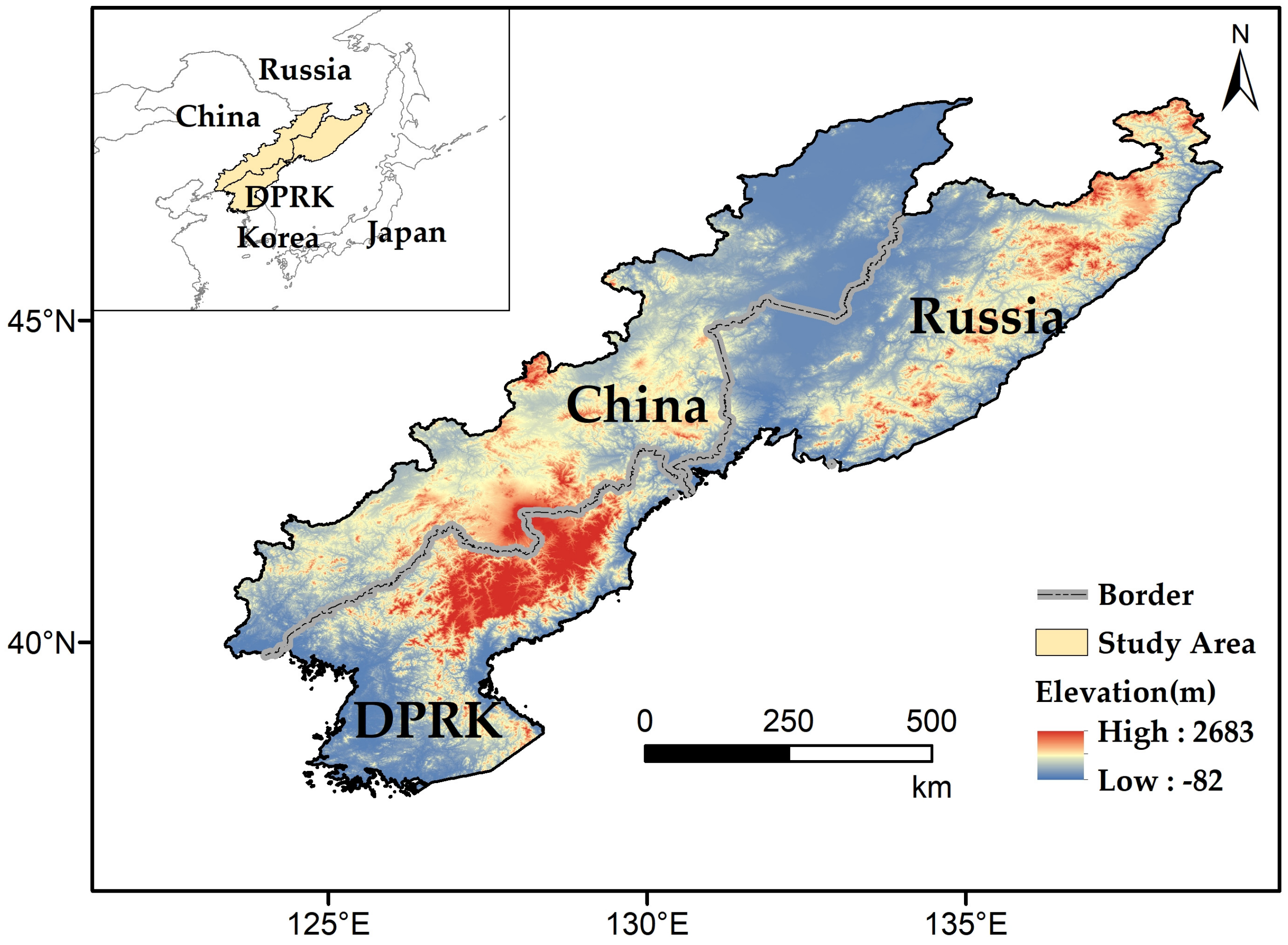
2.1. Study Area
2.2. Data
2.2.1. NDVI Data
2.2.2. Climate Data
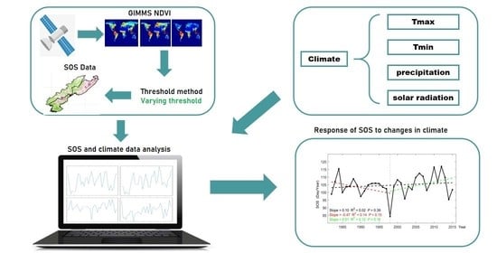
2.3. Methods
2.3.1. Extraction of SOS
2.3.2. Trend Analysis
2.3.3. Correlation Analysis of SOS and Climate Factors
3. Results and Discussion
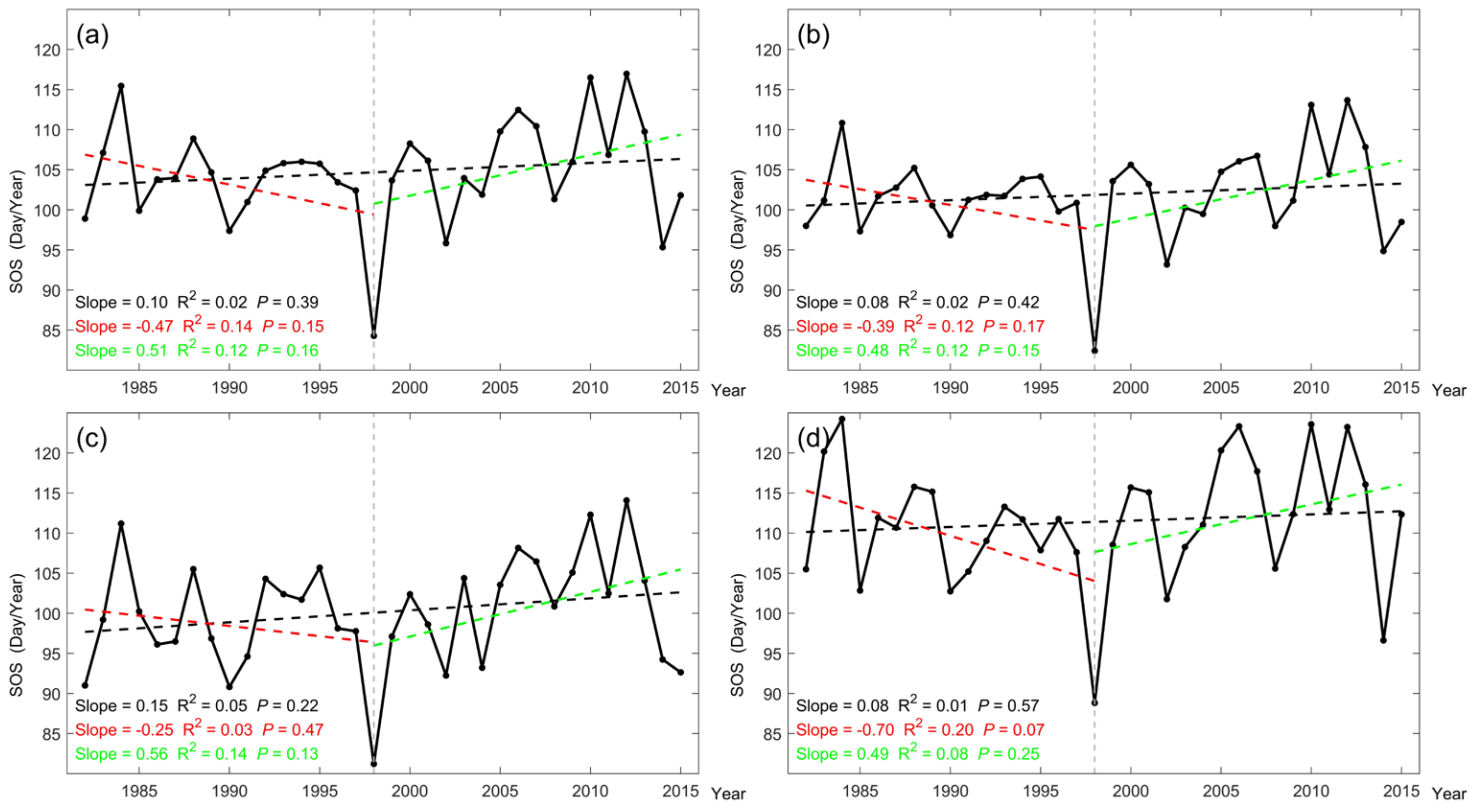
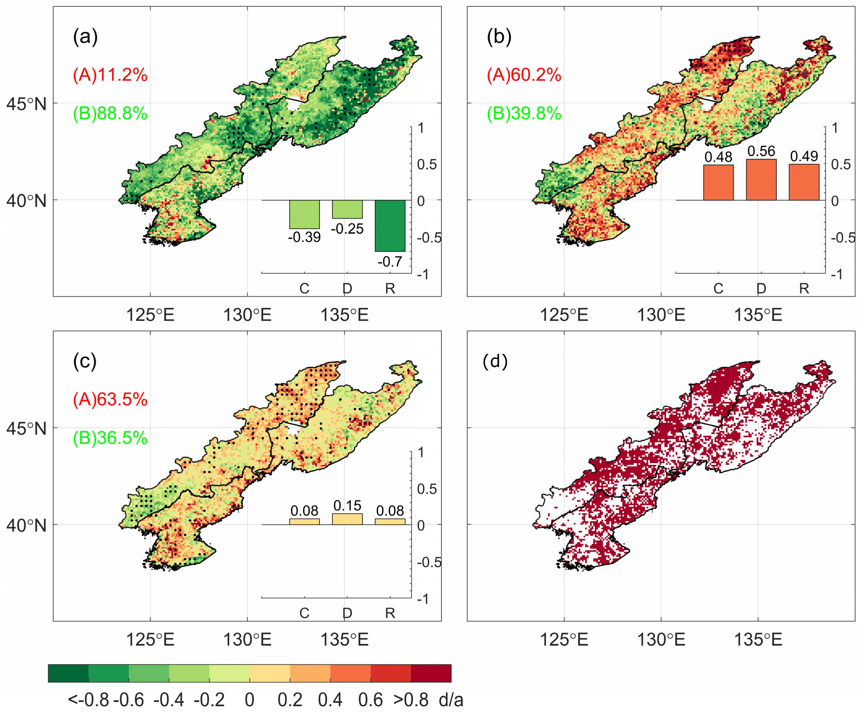
3.1. The Spatiotemporal Pattern of Spring Phenology
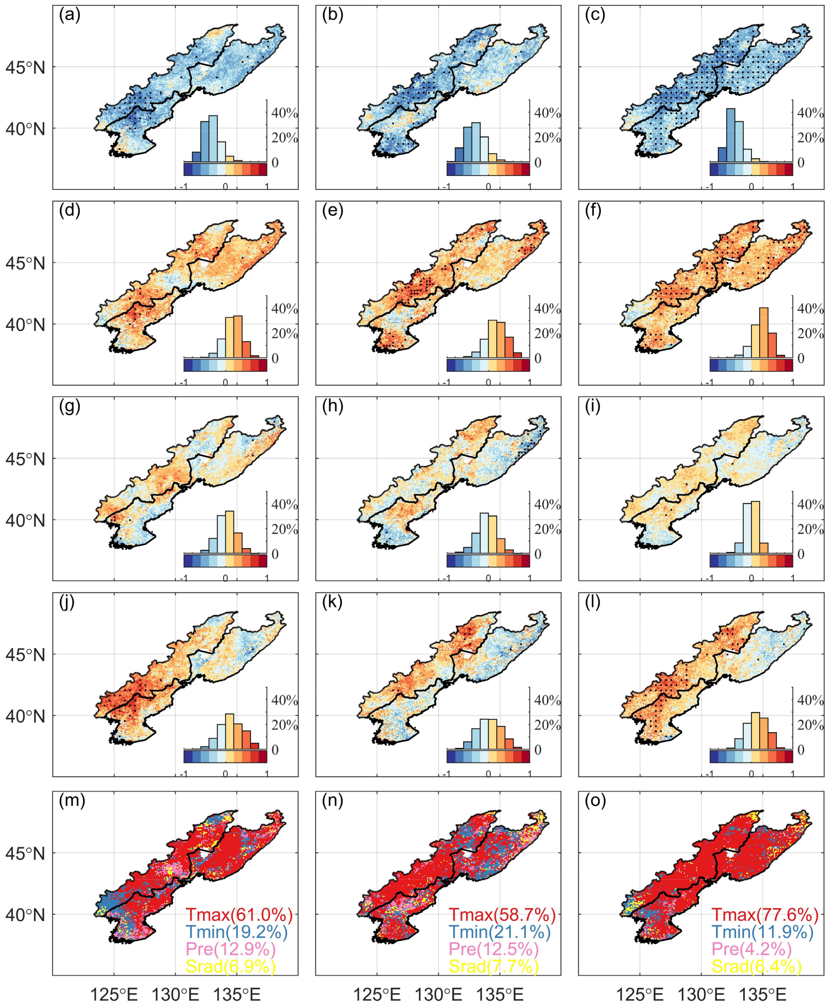
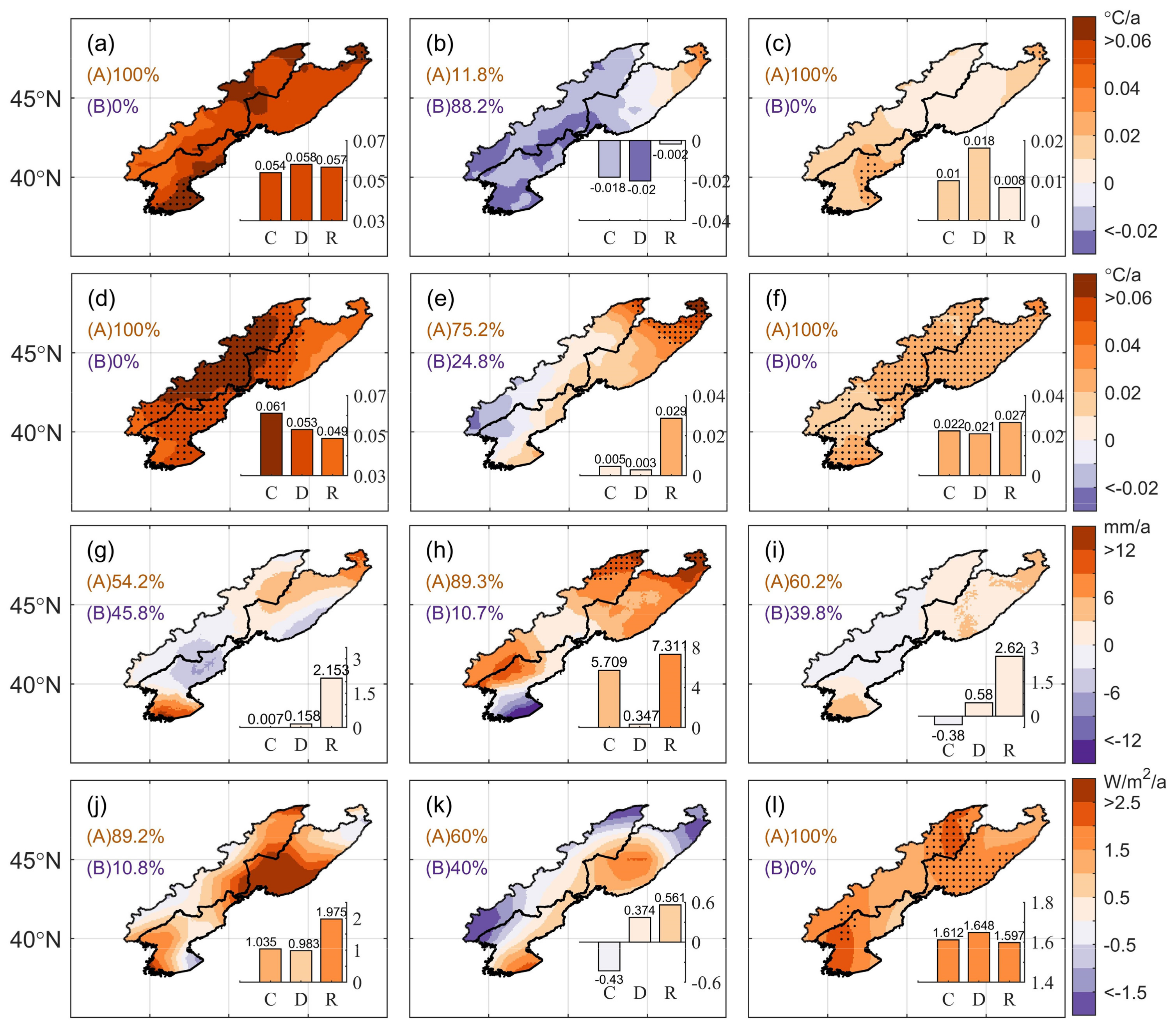
3.2. Impact of Climate Change on SOS
4. Conclusions
Author Contributions
Funding
Data Availability Statement
Acknowledgments
Conflicts of Interest
References
- Henebry, G.M.; Beurs, K.M.D. Remote Sensing of Land Surface Phenology: A Prospectus; Springer: Dordrecht, The Netherlands, 2013; pp. 385–411. [Google Scholar]
- Rodriguez-Galiano, V.F.; Dash, J.; Atkinson, P.M. Characterising the Land Surface Phenology of Europe Using Decadal MERIS Data. Remote Sens. 2015, 7, 9390–9409. [Google Scholar] [CrossRef] [Green Version]
- Piao, S.; Liu, Q.; Chen, A.; Janssens, I.; Fu, Y.; Dai, J.; Liu, L.; Lian, X.; Shen, M.; Zhu, X. Plant phenology and global climate change: Current progresses and challenges. Glob. Chang. Biol. 2019, 25, 1922–1940. [Google Scholar] [CrossRef] [PubMed]
- Myneni, R.; Keeling, C.D.; Tucker, C.J.; Asrar, G.; Nemani, R. Increased plant growth in the northern high latitudes from 1981 to 1991. Nature 1997, 386, 698–702. [Google Scholar] [CrossRef]
- Jochner, S.; Menzel, A. Does flower phenology mirror the slowdown of global warming? Ecol. Evol. 2015, 5, 2284–2295. [Google Scholar] [CrossRef]
- Pearson, R.G.; Phillips, S.J.; Loranty, M.M.; Beck, P.S.A.; Damoulas, T.; Knight, S.J.; Goetz, S.J. Shifts in Arctic vegetation and associated feedbacks under climate change. Nat. Clim. Chang. 2013, 3, 673–677. [Google Scholar] [CrossRef]
- Thackeray, S.J.; Henrys, P.A.; Hemming, D.; Bell, J.R.; Botham, M.S.; Burthe, S.; Helaouët, P.; Johns, D.G.; Jones, I.D.; Leech, D.I.; et al. Phenological sensitivity to climate across taxa and trophic levels. Nature 2016, 535, 241–245. [Google Scholar] [CrossRef] [Green Version]
- Zeng, Z.; Piao, S.; Li, L.Z.X.; Zhou, L.; Ciais, P.; Wang, T.; Li, Y.; Lian, X.; Wood, E.F.; Friedlingstein, P.; et al. Climate mitigation from vegetation biophysical feedbacks during the past three decades. Nat. Clim. Chang. 2017, 7, 432–436. [Google Scholar] [CrossRef]
- Lang, W.; Chen, X.; Qian, S.; Liu, G.; Piao, S. A new process-based model for predicting autumn phenology: How is leaf senescence controlled by photoperiod and temperature coupling? Agric. For. Meteorol. 2019, 268, 124–135. [Google Scholar] [CrossRef]
- Schwartz, M.D. Green-wave phenology. Nature 1998, 394, 839–840. [Google Scholar] [CrossRef]
- Ahas, R.; Jaagus, J.; Aasa, A. The phenological calendar of Estonia and its correlation with mean air temperature. Int. J. Biometeorol. 2000, 44, 159–166. [Google Scholar] [CrossRef]
- Menzel, A.; Fabian, P. Growing season extended in Europe. Nature 1999, 397, 659. [Google Scholar] [CrossRef]
- Peñuelas, J.; Filella, I. Responses to a Warming World. Science 2001, 294, 793–795. [Google Scholar] [CrossRef]
- Tucker, C.J.; Slayback, D.; Pinzon, J.E.; Los, S.; Myneni, R.; Taylor, M.G. Higher northern latitude normalized difference vegetation index and growing season trends from 1982 to 1999. Int. J. Biometeorol. 2001, 45, 184–190. [Google Scholar] [CrossRef]
- Zhou, L.; Tucker, C.J.; Kaufmann, R.K.; Slayback, D.; Shabanov, N.V.; Myneni, R.B. Variations in northern vegetation activity inferred from satellite data of vegetation index during 1981 to 1999. J. Geophys. Res. Atmos. 2001, 106, 20069–20083. [Google Scholar] [CrossRef]
- Lucht, W.; Prentice, I.C.; Myneni, R.B.; Sitch, S.; Friedlingstein, P.; Cramer, W.; Bousquet, P.; Buermann, W.; Smith, B. Climatic Control of the High-Latitude Vegetation Greening Trend and Pinatubo Effect. Science 2002, 296, 1687–1689. [Google Scholar] [CrossRef] [Green Version]
- Kimball, J.S.; McDonald, K.C.; Running, S.W.; Frolking, S.E. Satellite radar remote sensing of seasonal growing seasons for boreal and subalpine evergreen forests. Remote Sens. Environ. 2004, 90, 243–258. [Google Scholar] [CrossRef]
- Keeling, C.D.; Chin, J.F.S.; Whorf, T.P. Increased activity of northern vegetation inferred from atmospheric CO2 measurements. Nature 1996, 382, 146–149. [Google Scholar] [CrossRef]
- Fitter, A.H.; Fitter, R.S.R. Rapid Changes in Flowering Time in British Plants. Science 2002, 296, 1689–1691. [Google Scholar] [CrossRef]
- Roetzer, T.; Wittenzeller, M.; Haeckel, H.; Nekovar, J. Phenology in central Europe-differences and trends of spring phenophases in urban and rural areas. Int. J. Biometeorol. 2000, 44, 60–66. [Google Scholar] [CrossRef]
- Menzel, A.; Estrella, N.; Fabian, P. Spatial and temporal variability of the phenological seasons in Germany from 1951 to 1996. Glob. Change Biol. 2001, 7, 657–666. [Google Scholar]
- Sparks, T.H.; Roy, D.B.; Dennis, R.L.H. The influence of temperature on migration of Lepidoptera into Britain. Glob. Chang. Biol. 2005, 11, 507–514. [Google Scholar] [CrossRef]
- Chmielewski, F.-M.; Müller, A.; Bruns, E. Climate changes and trends in phenology of fruit trees and field crops in Germany, 1961–2000. Agric. For. Meteorol. 2004, 121, 69–78. [Google Scholar] [CrossRef]
- Richardson, A.D.; Bailey, A.S.; Denny, E.G.; Martin, C.W.; O’Keefe, J. Phenology of a northern hardwood forest canopy. Glob. Chang. Biol. 2006, 12, 1174–1188. [Google Scholar] [CrossRef] [Green Version]
- Xin-Bo, Z.; Jian-Ru, R.; Dan-Er, Z. Phenological observations onLarix principis-rupprechtii Mayr. in primary seed orchard. J. For. Res. 2001, 12, 201–204. [Google Scholar] [CrossRef]
- Piao, S.; Tan, J.; Chen, A.; Fu, Y.; Ciais, P.; Liu, Q.; Janssens, I.; Vicca, S.; Zeng, Z.; Jeong, S.-J.; et al. Leaf onset in the northern hemisphere triggered by daytime temperature. Nat. Commun. 2015, 6, 6911. [Google Scholar] [CrossRef] [Green Version]
- Shen, M.; Piao, S.; Chen, X.; An, S.; Fu, Y.H.; Wang, S.; Cong, N.; Janssens, I.A. Strong impacts of daily minimum temperature on the green-up date and summer greenness of the Tibetan Plateau. Glob. Chang. Biol. 2016, 22, 3057–3066. [Google Scholar] [CrossRef]
- Li, R.; Luo, T.; Mölg, T.; Zhao, J.; Li, X.; Cui, X.; Du, M.; Tang, Y. Leaf unfolding of Tibetan alpine meadows captures the arrival of monsoon rainfall. Sci. Rep. 2016, 6, 20985. [Google Scholar] [CrossRef]
- Shen, M.; Zhang, G.; Cong, N.; Wang, S.; Kong, W.; Piao, S. Increasing altitudinal gradient of spring vegetation phenology during the last decade on the Qinghai-Tibetan Plateau. Agric. For. Meteorol. 2014, 189, 71–80. [Google Scholar] [CrossRef]
- Yan, X.; Boyer, T.; Trenberth, K.; Karl, T.R.; Xie, S.; Nieves, V.; Tung, K.; Roemmich, D. The global warming hiatus: Slowdown or redistribution? Earth’s Future 2016, 4, 472–482. [Google Scholar] [CrossRef]
- IPCC. Climate Change 2013: The Physical Science Basis. Contribution of Working Group I to the Fifth Assessment Report of the Intergovernmental Panel on Climate Change; Cambridge Univ. Press: Cambridge, UK, 2013; 1535p. [Google Scholar]
- Jeong, S.J.; Chang-Hoi, H.O.; Gim, H.J.; Brown, M.E. Phenology shifts at start vs. end of growing season in temperate vegetation over the northern hemisphere for the period 1982–2008. Glob. Change Biol. 2011, 17, 2385–2399. [Google Scholar] [CrossRef]
- Park, H.; Jeong, S.-J.; Ho, C.-H.; Park, C.-E.; Kim, J. Slowdown of spring green-up advancements in boreal forests. Remote Sens. Environ. 2018, 217, 191–202. [Google Scholar] [CrossRef]
- Wang, X.; Xiao, J.; Li, X.; Cheng, G.; Ma, M.; Zhu, G.; Arain, M.A.; Black, T.A.; Jassal, R.S. No trends in spring and autumn phenology during the global warming hiatus. Nat. Commun. 2019, 10, 1–10. [Google Scholar] [CrossRef]
- Piao, S.; Fang, J.; Zhou, L.; Ciais, P.; Zhu, B. Variations in satellite-derived phenology in China’s temperate vegetation. Glob. Change Biol. 2006, 12, 672–685. [Google Scholar] [CrossRef]
- Shen, X.; Liu, B.; Jiang, M.; Wang, Y.; Wang, L.; Zhang, J.; Lu, X. Spatiotemporal Change of Marsh Vegetation and Its Response to Climate Change in China From 2000 to 2019. J. Geophys. Res. Biogeosci. 2021, 126, e2020JG006154. [Google Scholar] [CrossRef]
- Shen, X.; Liu, B.; Xue, Z.; Jiang, M.; Lu, X.; Zhang, Q. Spatiotemporal variation in vegetation spring phenology and its response to climate change in freshwater marshes of Northeast China. Sci. Total Environ. 2019, 666, 1169–1177. [Google Scholar] [CrossRef]
- Shen, X.; Liu, B.; Henderson, M.; Wang, L.; Wu, Z.; Wu, H.; Jiang, M.; Lu, X. Asymmetric effects of daytime and nighttime warming on spring phenology in the temperate grasslands of China. Agric. For. Meteorol. 2018, 259, 240–249. [Google Scholar] [CrossRef]
- Zhou, L.; Kaufmann, R.K.; Tian, Y.; Myneni, R.B.; Tucker, C.J. Relation between interannual variations in satellite measures of northern forest greenness and climate between 1982 and 1999. J. Geophys. Res. Atmos. 2003, 108, ACL-3. [Google Scholar] [CrossRef] [Green Version]
- Myneni, R.B.; Dong, J.; Tucker, C.J.; Kaufmann, R.K.; Kauppi, P.E.; Liski, J.; Zhou, L.; Alexeyev, V.; Hughes, M.K. A large carbon sink in the woody biomass of Northern forests. Proc. Natl. Acad. Sci. USA 2001, 98, 14784–14789. [Google Scholar] [CrossRef] [Green Version]
- Slayback, D.A.; Pinzon, J.E.; Los, S.O.; Tucker, C.J. Northern hemisphere photosynthetic trends 1982–99. Glob. Chang. Biol. 2003, 9, 1–15. [Google Scholar] [CrossRef]
- Shen, M.; Tang, Y.; Chen, J.; Zhu, X.; Zheng, Y. Influences of temperature and precipitation before the growing season on spring phenology in grasslands of the central and eastern Qinghai-Tibetan Plateau. Agric. For. Meteorol. 2011, 151, 1711–1722. [Google Scholar] [CrossRef]
- Piao, S.; Cui, M.; Chen, A.; Wang, X.; Ciais, P.; Liu, J.; Tang, Y. elevation and temperature dependence of change in the spring vegetation green-up date from 1982 to 2006 in the Qinghai-Xizang Plateau. Agric. For. Meteorol. 2011, 151, 1599–1608. [Google Scholar] [CrossRef]
- Ma, X.; Zhen, S.; Deng, J.; Feng, Q.; Huang, X. Vegetationphenology dynamics and its response to climate changeon the Tibetan Plateau. Acta Prataculturae Sin. 2016, 25, 13–21. [Google Scholar]
- Li Liu, L.; Zhang, Y.; Ding, M.; Li, S.; Chen, Q. Elevation-dependent alpine grassland phenology on the Tibetan Plateau. Geogr. Res. 2017, 36, 26–36. [Google Scholar]
- Wang, H.; Ge, Q.; Dai, J.; Tao, Z. Geographical pattern in first bloom variability and its relation to temperature sensitivity in the USA and China. Int. J. Biometeorol. 2014, 59, 961–969. [Google Scholar] [CrossRef]
- Cayan, D.R.; Dettinger, M.D.; Kammerdiener, S.A.; Caprio, J.M.; Peterson, D.H. Changes in the Onset of Spring in the Western United States. Bull. Am. Meteorol. Soc. 2001, 82, 399–415. [Google Scholar] [CrossRef] [Green Version]
- Lin, S.; Ge, Q.; Wang, H. Spatiotemporal change in leaf-out phenology of typicalEuropean tree species and its response to climate change. Chin. J. Appl. Ecol. 2021, 32, 788–798. [Google Scholar]
- Picard, G.; Quegan, S.; Delbart, N.; Lomas, M.R.; Toan, T.; Woodward, F.I. Bud-burst modelling in Siberia and its impact on quantifying the carbon budget. Glob. Chang. Biol. 2005, 11, 2164–2176. [Google Scholar] [CrossRef] [Green Version]
- Zheng, D.; Wallin, D.O.; Hao, Z. Rates and patterns of landscape change between 1972 and 1988 in the Changbai Mountain area of China and North Korea. Landsc. Ecol. 1997, 12, 241–254. [Google Scholar] [CrossRef]
- Tang, L.; Shao, G.; Piao, Z.; Dai, L.; Jenkins, M.A.; Wang, S.; Wu, G.; Wu, J.; Zhao, J. Forest degradation deepens around and within protected areas in East Asia. Biol. Conserv. 2010, 143, 1295–1298. [Google Scholar] [CrossRef]
- Lu, P.; Yu, Q.; He, Q. Plant Phenology Response to Climate Change. Acta Ecol. Sin. 2006, 26, 923–929. [Google Scholar]
- Zhang, H.; Li, Q.; Liu, J.; Shang, J.; Du, X.; Zhao, L.; Wang, N.; Dong, T. Crop classification and acreage estimation in North Korea using phenology features. GIScience Remote Sens. 2017, 54, 1–26. [Google Scholar] [CrossRef]
- Deng, G.; Zhang, H.; Guo, X.; Shan, Y.; Ying, H.; Rihan, W.; Li, H.; Han, Y. Asymmetric Effects of Daytime and Nighttime Warming on Boreal Forest Spring Phenology. Remote Sens. 2019, 11, 1651. [Google Scholar] [CrossRef] [Green Version]
- Meng, L.; Zhou, Y.; Li, X.; Asrar, G.R.; Mao, J.; Wanamaker, A.D.; Wang, Y. Divergent responses of spring phenology to daytime and nighttime warming. Agric. For. Meteorol. 2019, 281, 107832. [Google Scholar] [CrossRef]
- Fu, Y.H.; Liu, Y.; De Boeck, H.J.; Menzel, A.; Nijs, I.; Peaucelle, M.; Peñuelas, J.; Piao, S.; Janssens, I. Three times greater weight of daytime than of night-time temperature on leaf unfolding phenology in temperate trees. New Phytol. 2016, 212, 590–597. [Google Scholar] [CrossRef] [Green Version]
- Zhang, H.; Jin, Y.; Shen, X.; Li, G.; Zhou, D. Rising Air Temperature and Its Asymmetry under Different Vegetation Regions in China. Sci. Geogr. Sin. 2018, 38, 272–283. [Google Scholar]
- Zhang, P.; Shao, G.; Zhao, G.; Le Master, D.C.; Parker, G.R.; Dunning, J.B., Jr.; Li, Q. China’s forest policy for the 21st century. Science 2000, 288, 2135–2136. [Google Scholar] [CrossRef] [Green Version]
- Wang, X.; Piao, S.; Xu, X.; Ciais, P.; MacBean, N.; Myneni, R.B.; Li, L. Has the advancing onset of spring vegetation green-up slowed down or changed abruptly over the last three decades? Glob. Ecol. Biogeogr. 2015, 24, 621–631. [Google Scholar] [CrossRef]


| Year | Tmax/Contribution | Tmin/Contribution | Pre/Contribution | Srad/Contribution | |
|---|---|---|---|---|---|
| China | 1982–1998 | −0.36 (59.4%) | 0.16 (21.1%) | 0.08 (11.4%) | 0.25 (8.1%) |
| 1998–2015 | −0.40 (72.4%) | 0.25 (15.5%) | 0.03 (7.7%) | 0.18 (4.5%) | |
| 1982–2015 | −0.45 (83.1%) | 0.26 (9.2%) | 0.05 (1.7%) | 0.26 (6.0%) | |
| DPRK | 1982–1998 | −0.32 (48.9%) | 0.20 (25.3%) | −0.04 (19.9%) | 0.22 (6.0%) |
| 1998–2015 | −0.30 (53.8%) | 0.13 (18.3%) | −0.02 (17.4%) | −0.06 (10.4%) | |
| 1982–2015 | −0.33 (65.7%) | 0.19 (18.5%) | −0.02 (10.1%) | 0.17 (5.7%) | |
| Russia | 1982–1998 | −0.33 (71.4%) | 0.19 (12.8%) | 0.01 (9.6%) | −0.06 (6.2%) |
| 1998–2015 | −0.25 (45.5%) | 0.16 (30.0%) | −0.11 (14.7%) | −0.12 (9.9%) | |
| 1982–2015 | −0.39 (79.5%) | 0.49 (10.2%) | −0.06 (2.9%) | −0.06 (7.3%) |
Publisher’s Note: MDPI stays neutral with regard to jurisdictional claims in published maps and institutional affiliations. |
© 2022 by the authors. Licensee MDPI, Basel, Switzerland. This article is an open access article distributed under the terms and conditions of the Creative Commons Attribution (CC BY) license (https://creativecommons.org/licenses/by/4.0/).
Share and Cite
Su, M.; Huang, X.; Xu, Z.; Zhu, W.; Lin, Z. A Decrease in the Daily Maximum Temperature during Global Warming Hiatus Causes a Delay in Spring Phenology in the China–DPRK–Russia Cross-Border Area. Remote Sens. 2022, 14, 1462. https://doi.org/10.3390/rs14061462
Su M, Huang X, Xu Z, Zhu W, Lin Z. A Decrease in the Daily Maximum Temperature during Global Warming Hiatus Causes a Delay in Spring Phenology in the China–DPRK–Russia Cross-Border Area. Remote Sensing. 2022; 14(6):1462. https://doi.org/10.3390/rs14061462
Chicago/Turabian StyleSu, Minshu, Xiao Huang, Zhen Xu, Weihong Zhu, and Zhehao Lin. 2022. "A Decrease in the Daily Maximum Temperature during Global Warming Hiatus Causes a Delay in Spring Phenology in the China–DPRK–Russia Cross-Border Area" Remote Sensing 14, no. 6: 1462. https://doi.org/10.3390/rs14061462
APA StyleSu, M., Huang, X., Xu, Z., Zhu, W., & Lin, Z. (2022). A Decrease in the Daily Maximum Temperature during Global Warming Hiatus Causes a Delay in Spring Phenology in the China–DPRK–Russia Cross-Border Area. Remote Sensing, 14(6), 1462. https://doi.org/10.3390/rs14061462