Manifold-Based Multi-Deep Belief Network for Feature Extraction of Hyperspectral Image

Abstract

Deep belief networks (DBNs) have been widely applied in hyperspectral imagery (HSI) processing. However, the original DBN model fails to explore the prior knowledge of training samples which limits the discriminant capability of extracted features for classification. In this paper, we proposed a new deep learning method, termed manifold-based multi-DBN (MMDBN), to obtain deep manifold features of HSI. MMDBN designed a hierarchical initialization method that initializes the network by local geometric structure hidden in data. On this basis, a multi-DBN structure is built to learn deep features in each land-cover class, and it was used as the front-end of the whole model. Then, a discrimination manifold layer is developed to improve the discriminability of extracted deep features. To discover the manifold structure contained in HSI, an intrinsic graph and a penalty graph are constructed in this layer by using label information of training samples. After that, the deep manifold features can be obtained for classification. MMDBN not only effectively extracts the deep features from each class in HSI, but also maximizes the margins between different manifolds in low-dimensional embedding space. Experimental results on Indian Pines, Salinas, and Botswana datasets reach 78.25%, 90.48%, and 97.35% indicating that MMDBN possesses better classification performance by comparing with some state-of-the-art methods.

1. Introduction

Hyperspectral sensors can capture images in hundreds of narrow and continuous bands which provide fine spectral details for different ground objects, and hyperspectral image (HSI) has been widely used for various research fields, such as environmental science, geological science, urban planning, and precision agriculture [1,2,3,4]. In recent years, the analysis of HSI data has gained substantial attention and become an increasingly active research topic [5,6,7,8]. In real applications, it is a key task to classify each pixel in hyperspectral data [9,10,11]. However, the high dimensionality of HSI data generally leads to a problem named curse-of-dimensionality. While dimensionality reduction (DR) is an effective tool that can tackle this problem, it explores the transformation process from high-dimensional space to low-dimensional space to obtain embedding features [12,13].

In general, the DR methods can be categorized as feature selection (FS) and feature extraction (FE) [14,15]. The former is tried to search a subset of original variables for removing irrelevant or redundant features, while the latter projects data into low-dimensional embedding space and preserves most intrinsic information [16,17,18,19]. This paper mainly focuses on FE algorithms for dimensionality reduction of HSI.

The FE methods are divided into unsupervised, supervised, and semi-supervised ones [20,21]. Unsupervised FE algorithms learn low-dimensional features without exploring label information of training sets [22,23]. A number of unsupervised approaches have been proposed; such methods include principal component analysis (PCA) [24], locality preserving projections (LPP) [25,26], locally linear embedding (LLE) [27], neighborhood preserving embedding (NPE) [28], Laplacian eigenmaps (LE) [29], and local tangent space alignment (LTSA) [30]. However, the unsupervised nature limits the discriminant capability of embedding features for classification [31]. Supervised FE methods exploit prior knowledge of training samples to obtain discriminant features in low-dimensional space for classification [32,33], such as linear discriminant analysis (LDA) [34], locality sensitive discriminant analysis (LSDA) [35], local geometric structure Fisher analysis (LGSFA) [36], and marginal Fisher analysis (MFA) [37]. Although the aforementioned FE approaches may achieve good performance in some scenes, they heavily depend on shallow-based descriptors, which will limit the applicability of those methods in difficult scenes. The shallow features usually cannot deal with the nonlinear relationship between collected spectral information and corresponding land covers [38,39]. Therefore, extracting deep discriminant features is considered to be of great significance in HSI classification.

Recently, deep learning (DL) has been explored as an effective FE strategy to address nonlinear problems and it has shown the advantages in different fields such as natural language processing and computer vision [40,41,42,43]. Motivated by these encouraging applications, DL has been introduced into the classification of HSI [44,45,46,47]. Compared with the traditional shallow descriptors-based FE method, DL techniques can obtain discriminant information from original spectral features with hierarchical layers [48,49,50,51]. Chen et al. [52] designed a stacked autoencoder (SAE)-based method to classify the hyperspectral data by directly using spectral information in the DL model, and then learned features are classified by logistic regression. Chen et al. [53] extracted the deep features of HSI using convolutional neural network (CNN), and obtained high classification performance by spatial–spectral feature extraction. Li et al. [54] developed the manifold-based maximization margin discriminant network (M${}^3$DNet) to enhance the feature extraction ability of DL models. Although aforementioned deep models effectively explore deep features to enhance classification performance, they fail to consider the intrinsic manifold structure of HSI when constructing network models, which limits the discriminant ability of extracted features.

To address the above issues, a novel FE method termed manifold-based multi-deep belief network (MMDBN) is proposed by fusing deep network and manifold learning. MMDBN developed a new network initialization method based on local geometric structure among samples, and then built a multi-DBN model by training multiple DBNs with samples from each class to learn intrinsic information in different classes. After that, deep features extracted from the multi-DBN model are exploited to construct a discrimination manifold layer. In the manifold layer, a penalty graph and an intrinsic graph are explored to reveal the manifold structure of deep features for HSI data, which can further enhance the interclass separability and intraclass compactness in low-dimensional embedding space.

The contributions of the proposed approach are concluded as follows:

• A hierarchical initialization strategy is designed to utilize the local geometric structure to initialize the network;
• A multi-DBN structure is proposed to learn deep features from samples in each class, and the extracted abstract features are conducive to representing the deep information in hyperspectral data;
• A discrimination manifold layer is constructed by using the prior knowledge of training samples, and this will reveal the intrinsic manifold structure of deep features and bring the benefit to improve the discriminant capability of embedding features.

The remainder of this paper is organized as follows: A brief description of RBM, DBN, and graph embedding framework are presented in Section 2. Section 3 describes the proposed algorithm in detail. Section 4 gives experimental results to demonstrate the effectiveness of the MMDBN. We summarize this paper and provide recommendations for future work in Section 5.

2. Related Works

Let us denote a hyperspectral dataset by $X=[x_1,x_2,x_3,\cdots ,x_n]\in {\Re }^{D\times N}$, where N is the number of pixels and D indicates the number of spectral bands. The class label of $x_i$ is denoted by $l(x_i)=\{1,2,\cdots ,c\}$, and c is the class number of land covers. The purpose of FE is to learn a low-dimensional space $Z=[z_1,z_2,z_3,\cdots ,z_n]\in {\Re }^{d\times N}$, where d$(d\ll D)$ is the dimension of embedding features.

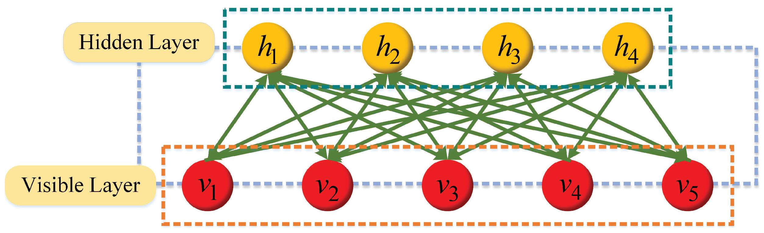
2.1. Restricted Boltzmann Machine (RBM)

RBM consists of visible a layer and a hidden layer. The visible layer is responsible for input, and the hidden layer learns high-level semantic features from input data. The visible unit and hidden unit are binary variables whose state is 1 or 0. The whole network is a bipartite graph, and there is no joining edge inside the visible layer or hidden layer, which exists between the visible unit $v=[v_1,\cdots ,v_m,\cdots ,v_k]$ and the hidden unit $h=[h_1,\cdots ,h_m,\cdots ,h_k]$. Figure 1 displays the network structure of RBM.

As an energy-based model, the joint configuration energy of visible unit v and hidden unit h for RBM is defined as follows:

$$E(v,h;\theta )=-\sum _m{b}_m{v}_m-\sum _n{a}_n{h}_n-\sum _{mn}{w}_{mn}{v}_m{h}_n$$

(1)

where $\theta =(w_{mn},a_n,b_m)$ is the parameter of RBM, $a_n$ and $b_m$ define the bias vectors of the hidden unit and visible unit, respectively, and $w_{mn}$ is the weight between visible unit $v_m$ and hidden unit $h_n$.

The joint probability distribution of v and h is calculated by

$$P(v,h;\theta )=\frac{1}{Z(\theta )}{e}^{-E(v,h;\theta )}$$

(2)

in which $Z(\theta )={\displaystyle \sum _v}{\displaystyle \sum _h}E(v,h;\theta )$ is the normalization factor.

The likelihood function of v and h are given as

$$P(h_n=1|v)=g(\sum _{m=1}{w}_{mn}{v}_m+a_n)$$

(3)

$$P(v_m=1|h)=g(\sum _{n=1}{w}_{mn}{h}_n+b_m)$$

(4)

where $g(x)=1/(1+exp(-x))$ is the logistic function.

The RBM model is trained by iteration, and the parameter $\theta =(w_{mn},a_n,b_m)$ can be obtained through the following gradient descent algorithm:

$$\theta =\theta +\eta \times \frac{\partial ln\left[{\displaystyle \prod _{m=1}^k}p(v|\theta )\right]}{\partial \theta }$$

(5)

where $\eta$ is a learning rate. With high-dimensional data, the gradient descent method is difficult to solve the model expectation. However, the training efficiency of RBM can greatly improve by using the contrastive divergence (CD) algorithm [55] as

$${(v_m{h}_n)}_{{}_{data}}-{(v_m{h}_n)}_{{}_{rec}}=\frac{\partial lnp(v|\theta )}{\partial w_{mn}}$$

(6)

where ${(•)}_{{}_{data}}$ indicates the mathematical expectation of training data, and ${(•)}_{{}_{rec}}$ represents the expectation of the reconstructed model. Then, the updated criteria for obtaining the DBN weight and bias are defined as follows:

$$\Delta w_{mn}=\eta ({(v_m{h}_n)}_{{}_{data}}-{(v_m{h}_n)}_{{}_{rec}})$$

(7)

$$\Delta a_m=\eta ({(v_m)}_{{}_{data}}-{(v_m)}_{{}_{rec}})$$

(8)

$$\Delta b_n=\eta ({(h_n)}_{{}_{data}}-{(h_n)}_{{}_{rec}})$$

(9)

After that, the parameters of RBM can be adjusted to the appropriate values to avoid the local optimal solution. RBM has a strong feature learning ability, and it can be used for information extraction. However, the performance of RBM for FE is limited when it is applied to complex nonlinear data.

2.2. Deep Belief Network (DBN)

To improve the representation ability of a single RBM, a DBN model is established by stacking multiple RBMs together. Thus, the DBN can explore a deep hierarchical representation of training samples. Figure 2 shows the structure of DBN.

As in Figure 2, the two adjacent layers of DBN can be considered as a single RBM. Every RBM is trained by the greedy layer-wise unsupervised learning, and an RBM does not consider other RBMs during its learning process [56].

2.3. Graph Embedding (GE)

The GE framework is designed to unify most classical DR approaches [37]. GE explores the desirable geometrical or statistical properties through an intrinsic graph $G(X,W)$ and avoids undesirable characteristics by a penalty graph $G_p(X,W^p)$, where X represents the vertex set of a graph. Both G and $G_P$ are undirected weighted graphs, W and $W^p$ are the weight matrices of two graphs, in which $w_{ij}$ measures the similarity between vertices $x_i$ and $x_j$ in intrinsic graph, and $w_{ij}^p$ calculates the dissimilarity of vertices $x_i$ and $x_j$ in penalty graph.

The similarity relationship between vertex pairs should be preserved in low-dimensional embedding space, and the objective function can be designed as

$$\begin{array}{c}\underset{Y^{T}HY=h}{argmin}\frac{1}{2}{\displaystyle \sum _{i=1}^n}{\displaystyle \sum _{j=1}^n}{\parallel y_i-y_j\parallel }^2{w}_{ij}=tr(Y^T(D-W)Y)=tr(Y^{T}LY)\hfill \end{array}$$

(10)

where h is a constant, D is a diagonal matrix, and $D_{ii}={\displaystyle \sum _{j=1}^N}{w}_{ij}$, L and H are Laplacian matrices of graph G and $G_p$. H is a constraint matrix for scale normalization, i.e., $H=L^p=D^p-W^p$, $D_{ii}^p={\displaystyle \sum _{j=1}^N}{w}_{ij}^p$.

3. Proposed Method

In this section, a manifold-based multi-deep belief network (MMDBN) is proposed to extract deep discriminant features for HSI classification. $X=[X_1,\cdots ,X_i,\cdots ,X_c]$ represents the hyperspectral dataset, where $X_i=[x_i^1,\cdots ,x_i^j,\cdots ,x_i^{N_i}]\in {\Re }^{D\times N_i}$ indicates the samples from the i-th class, and $N_i$ is the number of samples in it. $Y=[Y_1,\cdots ,Y_i,\cdots ,Y_c]$ represents the deep features extracted by multi-DBN structure, and $Y_i=[y_i^1,\cdots ,y_i^j,\cdots ,y_i^{N_i}]\in {\Re }^{D^{\prime }\times N_i}$ represents the features of corresponding class, where $D^{\prime }$ is the dimension of deep features. The output of MMDBN can be denoted as $z_i^j=A^T{y}_i^j$, where $A\in {\Re }^{D^{\prime }\times d}$ is the projection matrix and d is the dimension of low-dimensional features.

At first, MMDBN develops a local geometric structure-based initialization method and constructs a multi-DBN structure to train a DBN model for each class, then the deep features of different classes will be extracted with the corresponding DBN model. To further analyze the deep features extracted from the $(L-1)$-th layer, we designed a discrimination manifold layer as the last layer of the whole network. In this layer, the label information of each pixel is introduced as the prior knowledge to discover the manifold structure contained within hyperspectral data, and the layer separates the intermanifold samples while compacting the intramanifold samples, which increases the margins among different manifolds. Figure 3 displays the process of the MMDBN.

3.1. Local Geometric Structure-Based Network Initialization

Different from traditional DBN that initializes the network by random initialization, MMDBN develops a hierarchical initialization strategy based on the manifold structure in HSI.

Assume a DBN model consists of L layers, for i-th training labeled sample at l-th ($1\le l\le L$) layer, the output and input are $h_i^l$ and $v_i^l$, respectively. MMDBN builds a neighbor graph $G_n$ in each layer, $v_i^l$ is connected to samples from the same class, and the weights $s_{ij}^l$ are represented as

$$s_{ij}^l=exp(-{∥v_i^l-v_j^l∥}^2/\phantom{-{∥v_i^l-v_j^l∥}^{2}2{(t_i)}^2}2{(t_i)}^2)$$

(11)

where $s_{ij}^l$ is determined by the spectral Euclidean distance between the j-th and i-th training samples, and $t_i=\frac{1}{n}{\displaystyle \sum _{j=1}^n}∥v_i^l-v_j^l∥$ is the heat kernel parameter.

Given that $v_i^l$ and $v_j^l$ are neighbor points, we expect that the relationship can be maintained between $h_i^l$ and $h_j^l$. The corresponding objective function is represented by

$$R(M_l)=min(\frac{1}{2}\sum _{i=1}^N\sum _{j=1}^N{∥M_l{v}_i^l-M_l{v}_j^l∥}^2{s}_{ij}^l)$$

(12)

where $M_l$ is the network parameters matrix of layer l.

By some algebraic operations, Equation (12) can be reformulated as

$$\begin{array}{c}\frac{1}{2}{\displaystyle \sum _{i=1}^N}{\displaystyle \sum _{j=1}^N}{∥M_l{v}_i^l-M_l{v}_j^l∥}^2{s}_{ij}^l\hfill \\ =\frac{1}{2}tr({\displaystyle \sum _{i=1}^N}{\displaystyle \sum _{j=1}^N}(M_l{v}_i^l{s}_{ij}^l{(v_i^l)}^T{M}_l^T-2M_l{v}_i^l{s}_{ij}^l{(v_j^l)}^T{M}_l^T-M_l{v}_j^l{s}_{ij}^l{(v_j^l)}^T{M}_l^T))\hfill \\ =tr(M_l{V}^l(D^l-S^l){(V^l)}^T{M}_l^T)\hfill \\ =tr(M_l{V}^l{L}_l{(V^l)}^T{M}_l^T)\hfill \end{array}$$

(13)

in which $S^l={[s_{ij}^l]}_{i,j=1}^N$, $D^l=diag([{\displaystyle \sum _{j=1}^N}{s}_{ij}^l{]}_{i=1}^N)$.

To reduce the influence of scaling factors in the projection, a constraint $M_l{v}^l{(v^l)}^T{M}_l^T=I$ is imposed on the following objective function:

$$\left\{\begin{array}{c}min(tr(M_l{V}^l{L}_l{(V^l)}^T{M}_l^T))\\ s.t.M_l{V}^l{(V^l)}^T{M}_l^T=I\end{array}\right.$$

(14)

By introducing the Lagrange multiplier method, the optimization program of Equation (14) is transformed to tackle a generalized eigenvalue issue:

$$V^l{L}_l{(V^l)}^T{M}_l^T=\lambda V^l{(V^l)}^T{M}_l^T$$

(15)

where $M_l$ consists of d smallest eigenvalues of Equation (15) corresponding to eigenvectors.

3.2. Multi-DBN Structure

In order to extract deep features for each class in hyperspectral image, we designed a multi-DBN structure to fully extract the information in each class. As illustrated in Figure 3, the 1st to $(L-1)$-th layers in MMDBN belong to a multi-DBN structure. According to the properties of HSI, Gaussian distribution is introduced to model the input data, which realizes real-valued RBM instead of binary RBM [57,58]. The energy function and conditional probability distributions are defined as follows:

$$\begin{array}{c}E(v,h;\theta )=-{\displaystyle \sum _{m=1}}\frac{{(v_m^i-b_m^i)}^2}{2{({\sigma }_m^i)}^2}-{\displaystyle \sum _{n=1}}{a}_n^i{h}_n^i-{\displaystyle \sum _{m=1}}{\displaystyle \sum _{n=1}}{w}_{mn}^i\frac{v_m^i}{{\sigma }_m^i}{h}_n^i\hfill \end{array}$$

(16)

$$P(h_n^i|v_i;\theta )=g(\sum _{m=1}{w}_{mn}^i{v}_m^i+a_n^i)$$

(17)

$$P(v_n^i|h_i;\theta )=N(b_m^i+{\sigma }_m^i\sum _{j=1}{h}_n^i{w}_{mn}^i,{({\sigma }_m^i)}^2)$$

(18)

where ${\sigma }_i$ is the standard deviation of Gaussian visible units, and $N(\mu ,{\sigma }^2)$ is the Gaussian distribution with mean $\mu$ and variance $\sigma$.

The multi-DBN structure extracts features from the perspective of deep learning, and the features obtained from the $(L-1)$-th layer contain deep abstract information for hyperspectral data. To improve the discriminative capability of extracted features, MMDBN explores the manifold structure in HSI using label information.

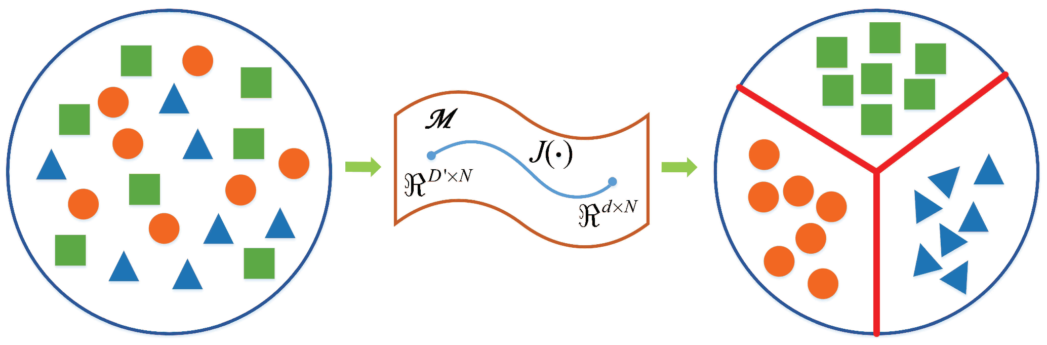
3.3. Discrimination Manifold Layer

The discrimination manifold layer allows the proposed method to discover the manifold structure in deep features, so that the extracted features can maintain large margins between different manifolds in low-dimensional embedding space. Figure 4 displays the illustration of the discrimination manifold layer.

The motivation of designing the discrimination manifold layer is to keep local geometric neighboring relation and label information in low-dimensional embedded space. To achieve this goal, it constructs the intra-DBN graph $G_w$ and the inter-DBN graph $G_b$ to explore the discriminant manifold structure from deep features. The weights between $y_i$ and $y_j$ for $G_w$ is represented by

$$w_{ij}^w=\left\{\begin{array}{c}exp(-\frac{{∥y_i-y_j∥}^2}{2{(t_i)}^2}),y_i\in N_{{}_w}(y_j)or{y}_j\in N_w(y_i)\hfill \\ 0,otherwise\hfill \end{array}\right.$$

(19)

For graph $G_b$, the weight is defined as

$$w_{ij}^b=\left\{\begin{array}{c}exp(-\frac{{∥y_i-y_j∥}^2}{2{(t_i)}^2}),y_i\in N_b(y_j)or{y}_j\in N_b(y_i)\hfill \\ 0,otherwise\hfill \end{array}\right.$$

(20)

where $N_w(y_i)$ is the $k_w$ intra-DBN neighbors of $y_i$ and $N_b(y_i)$ indicates the $k_b$ inter-DBN neighbors of $y_i$.

The purpose of the discrimination manifold layer is to separate deep features extracted from different DBNs and compact features learned from the same DBN. The objective functions are represented as

$$J_1(A)=\sum _{i=1}^N\sum _{j=1}^N{∥A^T{y}_i-A^T{y}_j∥}^2{w}_{ij}^w$$

(21)

$$J_2(A)=\sum _{i=1}^N\sum _{j=1}^N{∥A^T{y}_i-A^T{y}_j∥}^2{w}_{ij}^b$$

(22)

With some mathematical operations, Equations (21) and (22) can be reduced as

$$\begin{array}{c}{\displaystyle \sum _{i=1}^N}{\displaystyle \sum _{j=1}^N}{∥A^T{y}_i-A^T{y}_j∥}^2{w}_{ij}^w\hfill \\ =tr({\displaystyle \sum _{i=1}^N}{\displaystyle \sum _{j=1}^N}(A^T{y}_i{w}_{ij}^w{(y_i)}^{T}A-2A^T{y}_i{w}_{ij}^w{(y_j)}^{T}A-A^T{y}_j{w}_{ij}^w{(y_j)}^{T}A))\hfill \\ =tr(A^{T}Y(D^w-W^w)Y^{T}A)\hfill \\ =tr(A^{T}Y{L}_1{Y}^{T}A)\hfill \end{array}$$

(23)

$$\begin{array}{c}{\displaystyle \sum _{i=1}^N}{\displaystyle \sum _{j=1}^N}{∥A^T{y}_i-A^T{y}_j∥}^2{w}_{ij}^b\hfill \\ =tr({\displaystyle \sum _{i=1}^N}{\displaystyle \sum _{j=1}^N}(A^T{y}_i{w}_{ij}^b{(y_i)}^{T}A-2A^T{y}_i{w}_{ij}^b{(y_j)}^{T}A-A^T{y}_j{w}_{ij}^b{(y_j)}^{T}A))\hfill \\ =tr(A^{T}Y(D^b-W^b)Y^{T}A)\hfill \\ =tr(A^{T}Y{L}_2{Y}^{T}A)\hfill \end{array}$$

(24)

where $W^w={[w_{ij}^w]}_{i,j=1}^N$, $D^w=diag([{\displaystyle \sum _{j=1}^N}{w}_{ij}^w{]}_{i=1}^N)$, $W^b={[w_{ij}^b]}_{i,j=1}^N$, $D^b=diag([{\displaystyle \sum _{j=1}^N}{w}_{ij}^b{]}_{i=1}^N)$.

As discussed above, the discriminant manifold layer not only preserves the local geometric structure of HSI, but also maximizes the margins between different manifolds. Therefore, it possesses a discriminant capability at low-dimensional space, and the optimization of the following objective functions is an acceptable criterion for selecting an appropriate projection matrix:

$$\left\{\begin{array}{c}mintr(A^{T}Y{L}_1{Y}^{T}A)\\ maxtr(A^{T}Y{L}_2{Y}^{T}A)\end{array}\right.$$

(25)

The optimization problem of the multi-objective function in Equation (25) can be equivalent to

$$J(A)=min\frac{tr(A^{T}Y{L}_1{Y}^{T}A)}{tr(A^{T}Y{L}_2{Y}^{T}A)}$$

(26)

Then, the optimization solution can be formulated by Lagrange multiplier method into the following form:

$$\frac{\partial }{\partial A}tr(A^{T}Y{L}_1{Y}^{T}A-\lambda (A^{T}Y{L}_2{Y}^{T}A))=0$$

(27)

Based on the above mathematical transformation, Equation (27) can be further simplified as

$$Y{L}_1{Y}^{T}A=\lambda Y{L}_2{Y}^{T}A$$

(28)

where the optimal projection matrix $A=[a_1,a_2,\cdots ,a_d]$ consists of d eigenvectors corresponding to the d minimum eigenvalues of Equation (28). The low-dimensional embedding features are given as

$$Z=A^{T}Y\in {\Re }^{d\times N}$$

(29)

4. Experimental Results and Analysis

In this section, three real HSI datasets, Indian Pines, Salinas, and Botswana, are introduced to evaluate the effectiveness of the proposed MMDBN.

4.1. Experiment Datasets

Indian Pines dataset [59]: This dataset is a scene of Northwest Indiana acquired by the AVIRIS sensor. It contains 684 × 453 pixels with 220 bands, and its spatial resolution is 20 m. There are 200 radiance channels remaining after removing water vapor and atmospheric effect. It has 16 classes of land covers in total, and its false-color image and ground truth with detailed type information are given in Figure 5. Brackets list the sample size of each class.

Salinas dataset [59]: The second dataset was captured in Salinas Valley, Southern California through the AVIRIS sensor. The set is composed of 224 spectral channels after the 20 bands were removed due to the noise and water absorption. The spatial size of this dataset is up to 512 × 217 pixels, and its geometric resolution is 3.7 m. There are sixteen land cover types and the ground truth with corresponding classes are displayed in Figure 6.

Botswana dataset [59]: This dataset is a scene of Botswana Okavango Delta, South Africa collected by the Hyperion sensor on NASA EO-1 satellite on 31 May 2001. The size of the image is 1476 × 256 pixels and the spatial resolution is 30 m. A total of 145 spectral bands are utilized for the experiments after removing 20 channels seriously affected by noise. Figure 7 exhibits its false-color image and ground truth.

4.2. Experimental Setup

In all experiments, each HSI dataset was randomly divided into training and test set. Meanwhile, we set 10 training samples per class for small classes such as $Grass/pasture-mowed$, $Oats$, and $Alfalfa$ in Indian Pines dataset. A low-dimensional embedding space was constructed through DR method with the training samples, while the test set was mapped into the embedding space. Then, the K-nearest neighborhood (KNN) classifier with Euclidean distance was employed for classification. After that, $kappa$ coefficient ($Kappa$), average accuracy (AA), overall accuracy (OA), and classification accuracy for each class (CA) were introduced to investigate the performance of different DR approaches. Under each condition, the experiment was repeated 10 times to obtain a result with mean and standard deviation (STD). Experiments in this paper were completed on a computer with MATLAB 2014b, 32 GB memory, and i7-7800X CPU. The deep learning toolbox in MATLAB was used as a toolkit to develop the code of MMDBN.

4.3. Parameter Sensitivity Analysis

To evaluate the influence of parameters on the performance for MMDBN, 10%, 2%, and 10% samples in Indian Pines, Salinas, and Botswana datasets were randomly selected in each class of ground object for training, and the remaining samples were utilized for test.

4.3.1. Evaluation of the Model with Embedding Dimension

In this subsection, a series of experiments were designed to analyze the influence of embedding dimension for all FE algorithms. Figure 8 displays the OAs with different embedding dimensions.

As shown in Figure 8, the OAs of all algorithms first improve with the increase of embedding dimension, because there is more information that can be used for classification. However, the classification results for most algorithms tend to be stable or even reduced when the dimension reaches a certain degree, for the reason that valuable information contained in embedding features is close to saturation. Compared with other approaches, MMDBN achieved the best performance on all datasets, because it fuses multi-DBN structure and discrimination manifold layer to extract deep manifold features, which possesses a good discriminant ability for HSI classification. Based on the above analysis, we chose 30 as the feature dimension to achieve satisfactory performance. For LDA, the embedding dimension was set to $c-1$, in which c is the class number in HSI dataset.

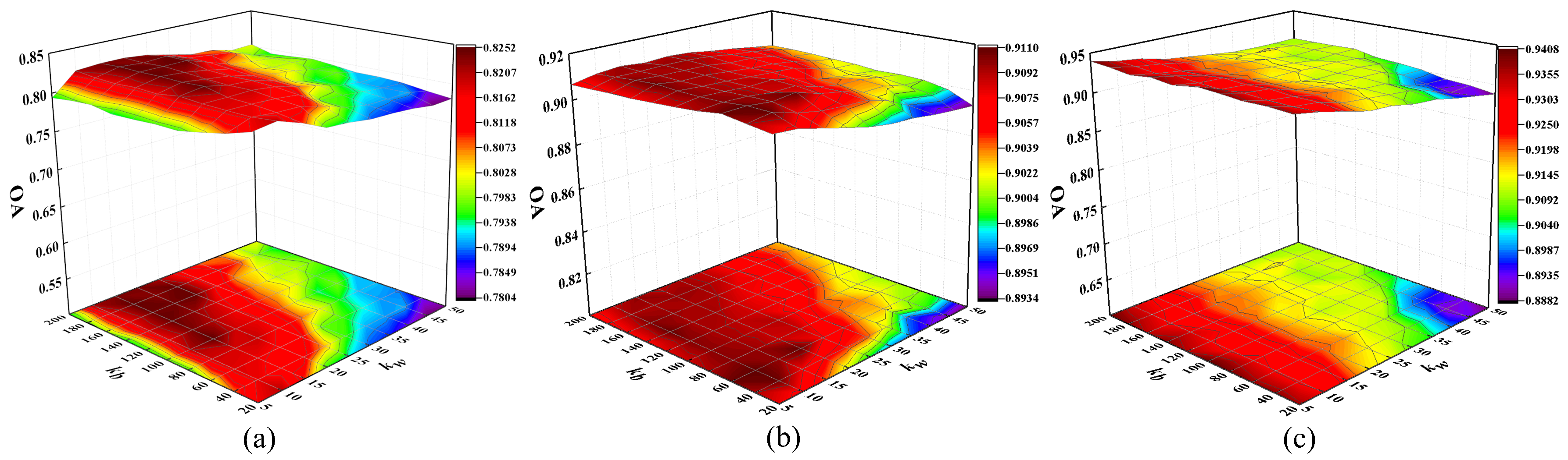
4.3.2. Evaluation of the Model with Different Value of Neighbors in Discrimination Manifold Layer

This subsection investigates the relationship between different number of interclass and intraclass neighbors and classification performance for the MMDBN method. In the experiment, parameters $k_b$ and $k_w$ are tuned with $\{20,40,60,\cdots ,200\}$ and $\{5,10,15,\cdots ,50\}$, respectively. The OAs with different values of $k_w$ and $k_b$ are shown in Figure 9.

From Figure 9, the OA improves and then stabilizes with the increase of $k_b$, because a large number of interclass neighbor points are conduciveto explore the discriminative structure for maximizing the manifold margins of HSI data. Meanwhile, an appropriate size of $k_w$ can discover the local manifold structure and compact samples from the same class. For three HSI datasets, we set the parameters $k_w$ and $k_b$ to 10 and 100, respectively.

4.3.3. Evaluation of the Model with Different Number of Model Layers

To analyze the impact with the number of layers on the performance of MMDBN, experiments were repeated ten times to obtain a result of OA with mean and standard deviation at each condition, and the relationship between the number of layers and the OAs on three HSI datasets are displayed in Figure 10.

As illustrated in Figure 10, the number of hidden layers within the multi-DBN structure plays a significant role in feature extraction of hyperspectral data. It can be easily observed that when the value of L is 3 or 4, the proposed approach will achieve better classification performance. This is because the parameter number in MMDBN increases dramatically with the increase of layer number, which easily leads to overfitting of limited training data. To obtain better classification results, the number of layers in MMDBN algorithm was set to 4 in three datasets.

4.3.4. Evaluation of the Model with Different Number of Nodes

To set a proper number of hidden nodes for the proposed model, we investigated the performance of MMDBN with a different number of nodes, and the nodes within each layer were tuned with $\{30,60,90,\cdots ,300\}$. Figure 11 shows the relationship between the node number in each layer and the classification accuracies.

According to Figure 11, nodes number has a considerable impact on the classification results of MMDBN. It can be easily observed that the OA first raises and then reduces. This indicates that too many nodes will bring negative effects for classification, and a high number of nodes will make the model redundant or even cause overlearning when limited training samples are available. Based on the above analysis, the optimal number of nodes is 60 for the three HSI datasets.

4.4. Comparisons with Other State-of-the-Art DR Methods

To evaluate the effectiveness of MMDBN, we compared it with several state-of-the-art DR approaches; such methods include Baseline, PCA [24], LDA [29], LPP [26], NPE [28], LGSFA [36], and MFA [37], and Baseline denotes that the test set is classified through KNN classifier without the process of DR. The cross-validation was adopted to obtain the optimal parameters for all methods. The number of neighbor points for LPP and NPE was chosen as 9. The numbers of intraclass and interclass neighbor points for LGSFA and MFA were set to 9 and 180, respectively.

In order to analyze the classification performance of each method with different size of training set, we selected $n_i(n_i=10,20,30,40,50,60,80,100)$ samples in each class for training, and the rest of the samples were set for test samples.

Table 1. The classification results of different DR algorithms for Indian Pines dataset (overall accuracy ± Std (%)).

Algorithm	${\mathit{n}}_{\mathit{i}}=10$	${\mathit{n}}_{\mathit{i}}=20$	${\mathit{n}}_{\mathit{i}}=30$	${\mathit{n}}_{\mathit{i}}=40$	${\mathit{n}}_{\mathit{i}}=50$	${\mathit{n}}_{\mathit{i}}=60$	${\mathit{n}}_{\mathit{i}}=80$	${\mathit{n}}_{\mathit{i}}=100$
Baseline	49.98 ± 1.91	55.49 ± 1.78	57.50 ± 2.12	58.99 ± 0.26	61.07 ± 0.50	61.51 ± 1.71	62.62 ± 0.91	63.74 ± 0.87
PCA	50.62 ± 2.41	55.04 ± 1.93	57.26 ± 0.82	58.70 ± 0.95	60.26 ± 0.20	61.89 ± 1.38	62.09 ± 1.01	63.45 ± 0.88
LDA	50.15 ± 2.22	51.18 ± 0.79	58.01 ± 1.16	62.24 ± 1.13	65.23 ± 1.03	66.44 ± 1.16	69.30 ± 0.94	71.01 ± 1.18
NPE	49.10 ± 2.02	53.09 ± 2.62	53.58 ± 0.90	56.99 ± 1.03	58.48 ± 0.43	59.98 ± 1.48	60.42 ± 0.65	61.72 ± 0.92
LPP	26.98 ± 6.92	45.73 ± 1.77	55.57 ± 1.07	57.18 ± 0.85	58.99 ± 0.43	60.68 ± 1.27	62.18 ± 0.67	64.04 ± 0.80
MFA	48.48 ± 1.77	54.11 ± 2.72	57.25 ± 1.24	58.50 ± 0.69	60.20 ± 0.85	62.49 ± 1.22	62.76 ± 1.22	65.67 ± 0.96
LGSFA	45.49 ± 3.47	56.71 ± 1.22	62.61 ± 1.33	67.18 ± 0.58	70.11 ± 1.61	71.84 ± 0.64	74.23 ± 0.98	75.63 ± 0.76
MMDBN	55.95 ± 3.65	64.06 ± 2.37	67.80 ± 2.21	71.21 ± 1.12	73.47 ± 0.92	75.30 ± 1.14	77.35 ± 0.69	78.25 ± 1.39

,

Table 2. The classification results of different DR algorithms for Salinas dataset (overall accuracy ± Std (%)).

Algorithm	${\mathit{n}}_{\mathit{i}}=10$	${\mathit{n}}_{\mathit{i}}=20$	${\mathit{n}}_{\mathit{i}}=30$	${\mathit{n}}_{\mathit{i}}=40$	${\mathit{n}}_{\mathit{i}}=50$	${\mathit{n}}_{\mathit{i}}=60$	${\mathit{n}}_{\mathit{i}}=80$	${\mathit{n}}_{\mathit{i}}=100$
Baseline	79.56 ± 2.45	81.91 ± 0.46	83.18 ± 1.07	83.42 ± 0.62	84.73 ± 0.90	84.81 ± 0.49	84.91 ± 1.01	85.20 ± 0.43
PCA	79.19 ± 2.39	82.89 ± 0.60	83.44 ± 0.85	83.82 ± 0.71	84.07 ± 0.77	84.37 ± 0.83	84.70 ± 0.78	84.93 ± 0.30
LDA	83.03 ± 1.72	84.06 ± 1.23	85.48 ± 0.94	87.62 ± 0.70	88.02 ± 1.02	88.85 ± 0.50	88.92 ± 0.89	89.09 ± 0.65
NPE	58.35 ± 3.17	81.28 ± 1.54	85.14 ± 1.06	85.43 ± 0.79	85.89 ± 0.98	86.15 ± 1.03	86.57 ± 1.11	86.68 ± 0.48
LPP	77.15 ± 2.60	81.83 ± 0.75	82.32 ± 0.66	83.05 ± 0.66	83.52 ± 0.91	83.91 ± 0.77	84.17 ± 0.81	84.50 ± 0.27
MFA	84.34 ± 1.93	86.57 ± 1.03	86.66 ± 0.37	86.91 ± 0.71	87.31 ± 0.81	87.58 ± 0.60	87.92 ± 1.44	88.66 ± 0.60
LGSFA	86.64 ± 1.01	87.20 ± 0.86	87.41 ± 0.49	87.89 ± 0.91	88.24 ± 0.88	88.36 ± 0.73	88.51 ± 0.87	89.62 ± 0.45
MMDBN	86.82 ± 2.10	88.44 ± 0.84	89.02 ± 0.81	89.31 ± 0.94	89.61 ± 0.77	89.95 ± 0.57	90.11 ± 0.52	90.48 ± 0.38

and

Table 3. The classification results of different DR algorithms for Botswana dataset (overall accuracy ± Std (%)).

Algorithm	${\mathit{n}}_{\mathit{i}}=10$	${\mathit{n}}_{\mathit{i}}=20$	${\mathit{n}}_{\mathit{i}}=30$	${\mathit{n}}_{\mathit{i}}=40$	${\mathit{n}}_{\mathit{i}}=50$	${\mathit{n}}_{\mathit{i}}=60$	${\mathit{n}}_{\mathit{i}}=80$	${\mathit{n}}_{\mathit{i}}=100$
Baseline	82.91 ± 0.98	86.71 ± 0.71	87.87 ± 0.64	88.83 ± 0.35	90.03 ± 0.64	90.36 ± 0.44	91.21 ± 0.72	91.49 ± 0.48
PCA	81.14 ± 1.50	84.86 ± 0.66	87.26 ± 0.86	87.79 ± 0.89	88.00 ± 0.78	88.78 ± 0.40	89.12 ± 0.33	90.01 ± 0.55
LDA	24.67 ± 6.19	83.19 ± 1.33	90.38 ± 0.56	91.75 ± 0.78	92.64 ± 0.32	93.28 ± 0.40	93.76 ± 0.67	94.40 ± 0.58
NPE	78.17 ± 1.41	83.62 ± 1.03	86.12 ± 0.62	86.95 ± 1.06	87.51 ± 0.58	88.40 ± 0.39	88.74 ± 0.18	89.72 ± 0.65
LPP	21.40 ± 0.50	79.21 ± 2.31	85.41 ± 0.65	87.47 ± 0.15	88.34 ± 1.05	88.79 ± 0.82	89.12 ± 0.61	90.10 ± 0.88
MFA	88.05 ± 1.44	90.17 ± 0.30	91.65 ± 0.29	92.41 ± 0.85	92.74 ± 0.93	93.61 ± 0.77	94.32 ± 0.41	95.25 ± 0.31
LGSFA	78.75 ± 3.49	88.16 ± 0.77	91.36 ± 0.71	93.30 ± 0.68	93.58 ± 0.43	94.13 ± 0.63	95.47 ± 0.52	96.00 ± 0.43
MMDBN	87.12 ± 1.69	91.55 ± 1.04	93.16 ± 0.51	94.67 ± 0.39	95.70 ± 0.30	95.91 ± 0.40	96.35 ± 0.52	97.35 ± 0.28

report the mean OA with STD for different DR approaches on three HSI datasets.

As shown in Table 1, Table 2 and Table 3, the OAs of all methods raise with the increase in the sample size of the training set. The experiment results of supervised learning methods outperform unsupervised learning methods in most conditions, the reason is that prior knowledge of training data brings benefits to improve the discriminative ability of extracted features. The proposed approach produces the best classification results among all DR methods, especially when there are a few available training samples. This is because the MMDBN not only extracts deep abstract features, but also explores a discrimination manifold layer to reveal the manifold structure within HSI.

To investigate the classification performance of MMDBN on different types of land covers, 10%, 2%, and 10% samples in each class were randomly selected from three datasets for training.

Table 4. Classification results of each class samples via different DR methods for Indian Pines dataset (%).

Class	Samples		DR with KNN Classifier
	Train	Test	Baseline	PCA	LDA	NPE	LPP	MFA	LGSFA	MMDBN
1	10	36	61.11 ± 16.97	61.11 ± 16.97	48.33 ± 15.23	60.00 ± 20.00	49.44 ± 16.63	43.06 ± 14.06	53.61 ± 7.17	68.61 ± 8.27
2	143	1285	53.32 ± 2.23	53.18 ± 2.28	66.80 ± 1.57	50.87 ± 1.98	55.69 ± 2.50	55.27 ± 1.76	63.53 ± 2.46	72.94 ± 1.75
3	83	747	50.15 ± 2.41	49.95 ± 2.38	55.91 ± 1.91	46.78 ± 2.86	52.65 ± 2.70	49.91 ± 2.33	54.92 ± 2.27	68.08 ± 3.34
4	24	213	33.36 ± 5.54	33.46 ± 5.52	39.68 ± 7.74	32.63 ± 5.06	36.64 ± 4.15	31.89 ± 4.96	31.98 ± 5.22	49.17 ± 4.33
5	49	434	82.63 ± 2.39	82.54 ± 2.31	86.88 ± 0.81	78.94 ± 3.27	82.45 ± 2.29	81.18 ± 1.65	85.68 ± 1.71	90.14 ± 1.74
6	73	657	89.55 ± 2.30	89.46 ± 2.33	91.56 ± 2.78	86.44 ± 2.72	88.41 ± 2.44	89.44 ± 3.05	90.71 ± 2.88	94.33 ± 2.95
7	10	18	89.44 ± 4.86	89.44 ± 4.84	91.67 ± 7.52	90.00 ± 4.38	88.89 ± 5.86	88.89 ± 6.42	89.44 ± 7.61	91.11 ± 4.69
8	48	430	91.96 ± 2.00	91.89 ± 1.94	94.39 ± 2.82	91.45 ± 2.31	88.32 ± 1.36	90.70 ± 2.01	91.64 ± 2.22	97.39 ± 1.18
9	10	10	71.00 ± 18.53	70.00 ± 19.44	77.00 ± 12.52	61.00 ± 13.70	72.00 ± 14.76	72.00 ± 12.29	77.00 ± 14.94	82.00 ± 11.98
10	98	874	64.97 ± 4.34	64.80 ± 4.31	71.53 ± 3.15	62.67 ± 4.15	66.09 ± 3.23	64.04 ± 3.09	68.73 ± 3.78	74.75 ± 3.21
11	246	2209	69.82 ± 1.52	69.79 ± 1.47	75.13 ± 1.10	67.20 ± 1.79	71.47 ± 1.96	71.66 ± 1.50	74.17 ± 1.96	82.13 ± 1.41
12	60	533	41.69 ± 2.29	41.50 ± 2.32	60.73 ± 2.60	39.10 ± 2.98	43.11 ± 2.92	44.92 ± 2.15	54.22 ± 2.47	74.95 ± 4.59
13	21	184	87.14 ± 6.00	87.19 ± 5.99	96.27 ± 2.75	81.35 ± 8.06	85.20 ± 7.49	88.60 ± 7.11	92.06 ± 6.45	97.51 ± 2.28
14	127	1138	89.75 ± 1.89	89.70 ± 1.87	92.88 ± 2.25	89.52 ± 2.15	89.81 ± 2.02	89.18 ± 2.42	91.97 ± 2.26	94.02 ± 1.72
15	39	347	35.98 ± 2.93	35.81 ± 2.78	52.46 ± 3.44	30.38 ± 3.02	34.16 ± 3.99	37.63 ± 5.32	43.44 ± 3.74	55.58 ± 3.48
16	10	83	88.19 ± 3.25	88.18 ± 3.25	85.30 ± 3.00	87.71 ± 3.40	85.30 ± 3.05	83.74 ± 3.37	84.70 ± 2.73	88.43 ± 4.79
OA			67.71 ± 0.48	67.61 ± 0.48	74.80 ± 0.87	65.28 ± 0.63	68.47 ± 0.91	68.25 ± 0.63	72.43 ± 0.93	81.56 ± 0.87
AA			68.75 ± 1.76	68.63 ± 1.87	74.16 ± 1.96	66.00 ± 1.93	68.10 ± 1.96	67.63 ± 1.91	71.74 ± 1.65	80.07 ± 1.66
Kappa			0.63 ± 0.01	0.63 ± 0.01	0.71 ± 0.01	0.60 ± 0.01	0.64 ± 0.01	0.64 ± 0.01	0.69 ± 0.01	0.78 ± 0.01
FE time (s)			-	0.03	0.03	0.31	0.11	0.13	13.08	26.08
Classification time (s)			0.41	0.36	0.32	0.33	0.32	0.31	0.62	0.38

,

Table 5. Classification results of each class samples via different DR methods for Salinas dataset (%).

Class	Samples		DR with KNN Classifier
	Train	Test	Baseline	PCA	LDA	NPE	LPP	MFA	LGSFA	MMDBN
1	41	1968	97.27 ± 0.58	97.27 ± 0.58	99.58 ± 0.55	96.70 ± 0.69	98.81 ± 0.42	98.45 ± 0.63	99.67 ± 0.26	99.22 ± 0.35
2	75	3651	99.37 ± 0.30	99.37 ± 0.30	99.92 ± 0.04	99.25 ± 0.32	99.60 ± 0.21	99.67 ± 0.31	99.83 ± 0.18	99.90 ± 0.10
3	40	1936	95.77 ± 2.40	95.76 ± 2.40	98.14 ± 1.17	94.84 ± 2.45	98.19 ± 1.12	96.25 ± 1.90	97.83 ± 1.16	98.81 ± 1.17
4	28	1366	99.23 ± 0.86	99.23 ± 0.86	99.43 ± 0.31	99.11 ± 0.95	99.44 ± 0.51	99.63 ± 0.22	99.55 ± 0.21	99.48 ± 0.38
5	54	2624	99.22 ± 0.86	96.21 ± 0.84	98.19 ± 0.46	95.35 ± 0.70	97.10 ± 0.85	96.50 ± 1.69	98.10 ± 0.56	98.35 ± 0.59
6	80	3879	99.59 ± 0.19	99.59 ± 0.19	99.87 ± 0.12	99.46 ± 0.22	99.69 ± 0.14	99.78 ± 0.09	99.88 ± 0.08	99.89 ± 0.08
7	72	3507	99.12 ± 0.20	99.12 ± 0.20	99.75 ± 0.15	98.98 ± 0.24	99.25 ± 0.22	99.57 ± 0.20	99.82 ± 0.08	99.63 ± 0.19
8	226	11,045	71.64 ± 0.82	71.62 ± 0.79	76.53 ± 1.96	69.91 ± 1.35	73.86 ± 1.46	75.81 ± 2.59	80.05 ± 2.23	83.53 ± 1.55
9	125	6078	98.13 ± 0.45	98.14 ± 0.45	99.81 ± 0.22	97.64 ± 0.60	99.45 ± 0.20	99.60 ± 0.21	99.88 ± 0.12	99.80 ± 0.16
10	66	3212	86.17 ± 3.36	86.18 ± 3.36	95.85 ± 0.67	84.47 ± 3.38	91.92 ± 2.23	91.96 ± 2.48	94.99 ± 0.72	95.75 ± 0.94
11	22	1046	89.00 ± 4.50	88.97 ± 4.49	95.25 ± 2.76	88.18 ± 4.18	94.69 ± 2.45	92.33 ± 3.49	96.04 ± 2.76	95.98 ± 2.63
12	39	1888	99.06 ± 1.12	99.06 ± 1.12	99.56 ± 0.41	98.81 ± 1.19	99.62 ± 0.50	99.69 ± 0.22	99.95 ± 0.10	99.99 ± 0.02
13	19	897	97.77 ± 0.86	97.77 ± 0.86	98.76 ± 0.92	97.51 ± 0.86	98.20 ± 0.74	98.37 ± 0.63	98.97 ± 0.60	98.61 ± 0.77
14	22	1048	90.57 ± 2.13	90.57 ± 2.13	94.40 ± 1.82	90.01 ± 2.20	92.44 ± 2.33	93.09 ± 2.34	94.28 ± 1.75	94.71 ± 1.96
15	146	7122	59.91 ± 1.59	59.87 ± 1.55	67.17 ± 2.02	57.73 ± 1.70	65.08 ± 1.84	66.56 ± 2.81	67.82 ± 2.69	63.60 ± 2.55
16	10	83	93.97 ± 3.00	93.96 ± 3.00	98.60 ± 0.60	91.72 ± 3.21	96.96 ± 1.95	98.06 ± 0.84	98.64 ± 0.47	98.89 ± 0.35
OA			83.39 ± 0.29	86.38 ± 0.28	89.93 ± 0.30	85.34 ± 0.41	88.55 ± 0.36	89.11 ± 0.60	90.73 ± 0.31	91.96 ± 0.32
AA			92.05 ± 0.46	92.04 ± 0.46	95.05 ± 0.19	91.23 ± 0.50	94.02 ± 0.34	94.08 ± 0.38	95.32 ± 0.14	95.40 ± 0.16
Kappa			0.85 ± 0.00	0.85 ± 0.00	0.89 ± 0.00	0.84 ± 0.00	0.87 ± 0.00	0.88 ± 0.01	0.90± 0.00	0.90 ± 0.00
FE time (s)			-	0.05	0.03	0.26	0.13	0.15	3.91	19.49
Classification time (s)			2.51	2.38	2.31	2.36	2.34	2.29	3.38	5.39

and

Table 6. Classification results of each class samples via different DR methods for Botswana dataset (%).

Class	Samples		DR with KNN Classifier
	Train	Test	Baseline	PCA	LDA	NPE	LPP	MFA	LGSFA	MMDBN
1	27	243	99.91 ± 0.18	99.21 ± 0.18	100.00 ± 0.00	99.88 ± 0.28	99.96 ± 0.13	99.83 ± 0.53	99.88 ± 0.28	99.92 ± 0.26
2	11	90	86.70 ± 8.03	86.81 ± 7.98	96.15 ± 2.50	81.99 ± 9.75	82.86 ± 6.78	93.96 ± 5.75	95.60 ± 4.63	95.28 ± 4.86
3	26	225	94.97 ± 2.31	94.98 ± 2.31	97.74 ± 1.52	91.67 ± 3.84	96.24 ± 3.35	98.46 ± 0.68	98.41 ± 1.61	98.37 ± 1.40
4	22	193	93.28 ± 2.72	93.28 ± 2.72	96.94 ± 2.60	91.23 ± 2.34	96.41 ± 1.73	97.85 ± 1.25	97.95 ± 1.74	98.05 ± 1.49
5	27	242	75.94 ± 4.08	75.86 ± 4.10	85.52 ± 5.47	74.44 ± 3.92	75.36 ± 5.62	79.83 ± 5.17	85.02 ± 5.67	88.66 ± 4.76
6	27	242	59.54 ± 4.60	59.62 ± 4.55	75.73 ± 5.08	55.15 ± 3.07	59.33 ± 5.90	72.76 ± 5.54	75.02 ± 4.59	79.50 ± 4.68
7	26	233	97.03 ± 0.94	96.99 ± 1.02	98.87 ± 0.69	96.11 ± 1.34	97.90 ± 0.74	97.77 ± 1.26	98.60 ± 0.54	99.04 ± 0.54
8	21	182	94.10 ± 3.78	94.21 ± 3.72	94.10 ± 3.02	92.46 ± 3.65	91.42 ± 4.17	98.09 ± 1.79	93.66 ± 3.99	96.94 ± 2.22
9	32	282	77.47 ± 3.36	77.57 ± 3.41	83.45 ± 5.10	73.98 ± 3.65	74.12 ± 5.19	84.97 ± 2.88	86.66 ± 6.09	88.45 ± 3.38
10	25	223	84.04 ± 3.98	83.99 ± 3.88	90.18 ± 4.36	81.51 ± 4.82	83.62 ± 4.85	88.58 ± 5.01	89.77 ± 3.45	91.46 ± 3.59
11	31	274	89.49 ± 3.99	89.42 ± 3.94	90.66 ± 3.07	88.62 ± 4.13	87.16 ± 3.94	90.15 ± 4.61	91.20 ± 4.03	92.95 ± 3.77
12	19	162	92.24 ± 2.87	92.30 ± 2.89	88.51 ± 3.75	91.80 ± 2.11	91.93 ± 2.90	91.62 ± 3.06	91.93 ± 4.33	93.98 ± 2.17
13	27	241	86.01 ± 4.76	86.01 ± 4.75	88.91 ± 4.02	83.40 ± 5.77	86.72 ± 4.38	90.71 ± 3.19	89.50 ± 2.93	91.77 ± 2.77
14	10	85	98.00 ± 1.84	98.00 ± 1.84	93.18 ± 5.68	98.12 ± 1.86	96.94 ± 1.14	97.06 ± 2.17	94.71 ± 4.38	95.77 ± 3.10
OA			86.77 ± 1.84	86.78 ± 0.70	90.85 ± 0.58	84.71 ± 0.66	86.22 ± 0.57	90.75 ± 0.85	91.41 ± 0.50	94.01 ± 0.72
AA			87.77 ± 0.90	87.78 ± 0.89	91.43 ± 0.83	85.74 ± 0.81	87.14 ± 0.70	91.55 ± 0.83	91.99 ± 0.70	93.58 ± 0.78
Kappa			0.86 ± 0.01	0.86 ± 0.01	0.91 ± 0.01	0.83 ± 0.01	0.85 ± 0.01	0.90 ± 0.1	0.91 ± 0.01	0.92 ± 0.01
FE time (s)			-	0.01	0.03	0.06	0.05	0.35	3.13	3.70
Classification time (s)			0.06	0.07	0.03	0.04	0.04	0.03	0.09	0.04

list the classification accuracy of each class for different methods on HSI datasets, and corresponding classification maps are shown in Figure 12, Figure 13 and Figure 14, respectively.

As illustrated in Table 4, Table 5 and Table 6, the proposed approach achieves better classification results on most classes of three datasets, especially for the Indian Pines dataset. Compared with other methods without a multi-manifold model, MMDBN needs longer FE time because it learns the intrinsic information of each type of land cover by constructing a multi-DBN structure. However, it is acceptable owing to the competitive results of MMDBN. As displayed in Figure 12, Figure 13 and Figure 14, it is clear that the proposed approach generated more homogenous regions in classification maps than comparison methods. The results show that the MMDBN extracts the deep discriminant features of each class, and maximizes the manifold margins among different classes.

4.5. Comparisons with Some Deep Learning Methods

To further compare the performance of MMDBN with deep learning models, ANN [43], CNN [53], SAE [52], M${}^3$DNet [54], and MDBN were introduced as compared algorithms. MDBN means the multi-DBN structure without the discrimination manifold layer, and we set the parameters of each model empirically to achieve the best performance in each condition.

In experiments, the training set contained $n_i(n_i=20,40,60,80,100)$ samples randomly selected in each class, and the test set consisted of the remaining samples. The average OA with STD for different methods is given in

Table 7. The classification results for different deep learning methods (overall accuracy ± Std (%)).

	Algorithm	${\mathit{n}}_{\mathit{i}}$ = 20	${\mathit{n}}_{\mathit{i}}$ = 40	${\mathit{n}}_{\mathit{i}}$ = 60	${\mathit{n}}_{\mathit{i}}$ = 80	${\mathit{n}}_{\mathit{i}}$ = 100
Indian Pines	ANN	49.06 ± 4.38	56.79 ± 4.11	60.86 ± 5.82	81.78 ± 5.63	66.21 ± 4.07
	SAE	56.06 ± 2.37	65.22 ± 1.27	68.99 ± 1.85	71.24 ± 1.74	73.52 ± 1.01
	CNN	60.47 ± 2.11	68.19 ± 3.31	74.26 ± 2.82	76.76 ± 3.13	78.11 ± 2.52
	M${}^3$DNet	53.01 ± 2.59	60.89 ± 3.05	64.70 ± 4.15	65.39 ± 4.14	68.94 ± 2.74
	MDBN	56.05 ± 1.66	60.04 ± 1.14	63.96 ± 0.94	64.58 ± 0.87	65.02 ± 0.85
	MMDBN	64.06 ± 2.37	71.21 ± 1.12	75.30 ± 1.14	77.35 ± 0.69	78.25 ± 1.39
Salinas	ANN	83.12 ± 1.60	85.77 ± 1.16	87.03 ± 1.25	88.22 ± 1.04	88.25 ± 1.11
	SAE	83.95 ± 0.98	86.42 ± 1.05	87.82 ± 0.47	88.77 ± 0.79	88.74 ± 0.80
	CNN	78.55 ± 3.05	85.16 ± 2.32	86.03 ± 2.27	84.88 ± 4.71	89.02 ± 3.00
	M${}^3$DNet	83.96 ± 1.40	86.39 ± 1.16	87.50 ± 1.11	88.13 ± 1.75	88.53 ± 0.89
	MDBN	82.80 ± 1.44	83.23 ± 1.23	86.15 ± 0.55	86.41 ± 0.52	85.84 ± 0.67
	MMDBN	88.38 ± 1.66	89.31 ± 0.94	89.95 ± 0.57	90.11 ± 0.52	90.48 ± 0.38
Botswana	ANN	86.95 ± 1.62	88.53 ± 1.01	89.54 ± 1.28	91.00 ± 1.73	91.53 ± 1.04
	SAE	88.51 ± 1.61	91.53 ± 0.51	92.92 ± 0.90	93.64 ± 0.74	94.38 ± 0.54
	CNN	87.42 ± 4.82	92.66 ± 3.65	94.04 ± 3.50	96.45 ± 1.93	97.14 ± 2.17
	M${}^3$DNet	88.60 ± 1.66	90.11 ± 1.04	91.46 ± 1.00	92.69 ± 1.15	92.85 ± 0.73
	MDBN	89.21 ± 0.79	91.58 ± 0.59	93.39 ± 0.65	94.02 ± 0.55	94.33 ± 0.67
	MMDBN	91.55 ± 1.04	94.67 ± 0.39	95.91 ± 0.40	96.35 ± 0.52	97.35 ± 0.28

.

From Table 7, the classification accuracies of different deep learning models on three datasets are improved as the training samples increased, because a larger size of the training set can bring rich discriminant information for extracted features. Different from traditional deep learning methods, MMDBN initializes the network by exploring the local geometric structure. Meanwhile, it designs a multi-DBN structure to learn intrinsic information of different classes, and then improves the separability of features by constructing a discrimination manifold layer. As a result, the proposed approach achieves the best results in most cases. Compared with MDBN, the competitive performance of MMDBN shows the effectiveness of the discrimination manifold layer, and it can compact samples for the same class and separate samples for different classes; this is conducive to extracting discriminant features for land cover classification.

To investigate the running time of different deep learning methods, we randomly selected 10%, 2%, and 10% samples per class from three datasets for training and the rest of the data were chosen as a test set.

Table 8. Classification accuracy (%) and running time (seconds) of different deep learning models.

Dataset	Algorithm	Classification Accuracy (%)		Running Time (s)
		OA	Kappa	Train	Test
Indian Pines	ANN	66.11	60.65	301.25	0.06
	SAE	73.93	69.66	288.26	0.04
	CNN	80.41	77.70	568.03	5.51
	M${}^3$DNet	68.82	63.93	635.21	0.04
	MDBN	69.06	64.67	13.08	0.62
	MMDBN	81.50	78.61	26.08	0.38
Salinas	ANN	87.84	86.45	222.69	0.18
	SAE	89.62	88.44	197.23	0.14
	CNN	90.98	89.96	328.66	43.05
	M${}^3$DNet	88.03	88.03	429.70	0.18
	MDBN	87.45	86.03	3.91	3.38
	MMDBN	91.79	90.85	19.49	5.39
Botswana	ANN	86.52	85.38	36.11	0.03
	SAE	90.75	89.98	28.03	0.01
	CNN	92.73	92.11	125.05	2.03
	M${}^3$DNet	88.90	87.97	63.99	0.01
	MDBN	90.34	89.53	3.13	0.09
	MMDBN	94.06	93.56	3.70	0.04

lists Kappas, OAs, and running times for different methods on three datasets.

The running times of MDBN and MMDBN are significantly less than other deep learning models under the training phase. While in the test phase, the subsequent classification process of MMDBN needs to explore the k-nearest neighbors of extracted features, so it takes a longer time than some comparison methods.

5. Conclusions

The deep belief network (DBN) model is an unsupervised deep learning method and it fails to discover manifold structure in HSI. This paper proposes a novel FE method called MMDBN, which combines manifold learning and deep learning to address these issues. MMDBN extracts the deep abstract features contained in various land covers by constructing a multi-DBN structure. Then, under the GE framework, it designs the discrimination manifold layer for supervised learning, which can separate interclass samples while compactingintraclass samples. As a result, the proposed approach effectively extracts discriminant features and significantly improves classification accuracy for hyperspectral data. Experiment results on Indian Pines, Salinas, and Botswana HSI datasets show that the proposed MMDBN has a better ability for feature extraction than some state-of-the-art DR methods.

In the future, we are interested in exploring the spatial information of hyperspectral data to solve the limitation of MMDBN only considering spectral information, and designing the spectral–spatial combined deep manifold networks to further improve the classification performance of the MMDBN model.

References

1. Zhong, Z.L.; Li, J.; Clausi, D.A.; Wong, A. Generative Adversarial Networks and Conditional Random Fields for Hyperspectral Image Classification. IEEE Trans. Cybern. 2020, 50, 3318–3329. [Google Scholar] [CrossRef] [PubMed] [Green Version]
2. Luo, F.L.; Zhang, L.P.; Du, B. Dimensionality Reduction with Enhanced Hybrid-graph Discriminant Learning for Hyperspectral Image Classification. IEEE Trans. Geosci. Remote Sens. 2020, 58, 5336–5353. [Google Scholar] [CrossRef]
3. Zhong, Y.F.; Wang, X.Y.; Xu, Y.; Wang, S.Y.; Jia, T.Y.; Hu, X.; Zhao, J.; Wei, L.F.; Zhang, L.P. Mini-UAV-Borne Hyperspectral Remote Sensing: From Observation and Processing to Applications. IEEE Geosci. Remote Sens. Mag. 2018, 6, 46–62. [Google Scholar] [CrossRef]
4. Kuras, A.; Brell, M.; Rizzi, J.; Burud, I. Hyperspectral and Lidar Data Applied to the Urban Land Cover Machine Learning and Neural-Network-Based Classification: A Review. Remote Sens. 2021, 13, 3393. [Google Scholar] [CrossRef]
5. Vali, A.; Comai, S.; Matteucci, M. Deep Learning for Land Use and Land Cover Classification Based on Hyperspectral and Multispectral Earth Observation Data: A Review. Remote Sens. 2020, 12, 2495. [Google Scholar] [CrossRef]
6. Peng, J.T.; Li, L.Q.; Tang, Y.Y. Maximum Likelihood Estimation-Based Joint Sparse Representation for the Classification of Hyperspectral Remote Sensing Images. IEEE Trans. Neural Netw. Learn. Syst. 2019, 30, 1790–1802. [Google Scholar] [CrossRef] [PubMed]
7. Gao, H.M.; Yang, Y.; Li, C.M.; Gao, L.R.; Zhang, B. Multiscale Residual Network With Mixed Depthwise Convolution for Hyperspectral Image Classification. IEEE Trans. Geosci. Remote Sens. 2021, 59, 3396–3408. [Google Scholar] [CrossRef]
8. Zhang, X.R.; Gao, Z.Y.; Jiao, L.C.; Zhou, H.Y. Multifeature Hyperspectral Image Classification With Local and Nonlocal Spatial Information via Markov Random Field in Semantic Space. IEEE Trans. Geosci. Remote Sens. 2018, 56, 1409–1424. [Google Scholar] [CrossRef] [Green Version]
9. Su, H.J.; Zhao, B.; Du, Q.; Du, P.J. Kernel Collaborative Representation With Local Correlation Features for Hyperspectral Image Classification. IEEE Trans. Geosci. Remote Sens. 2019, 57, 1230–1241. [Google Scholar] [CrossRef]
10. Hong, D.F.; Yokoya, N.; Chanussot, J.; Zhu, X.X. An Augmented Linear Mixing Model to Address Spectral Variability for Hyperspectral Unmixing. IEEE Trans. Image Process. 2019, 28, 1923–1938. [Google Scholar] [CrossRef] [Green Version]
11. Jiao, C.Z.; Chen, C.; McGarvey, R.G.; Bohlman, S.; Jiao, L.C. Multiple Instance Hybrid Estimator for Hyperspectral Target Characterization and Sub-pixel Target Detection. ISPRS J. Photogramm. Remote Sens. 2018, 146, 235–250. [Google Scholar] [CrossRef] [Green Version]
12. Luo, F.L.; Du, B.; Zhang, L.P.; Zhang, L.F.; Tao, D.C. Feature Learning Using Spatial-Spectral Hypergraph Discriminant Analysis for Hyperspectral Image. IEEE Trans. Cybern. 2019, 49, 2406–2419. [Google Scholar] [CrossRef] [PubMed]
13. Huang, H.; Shi, G.Y.; He, H.B.; Duan, Y.L.; Luo, F.L. Dimensionality Reduction of Hyperspectral Imagery Based on Spatial-spectral Manifold Learning. IEEE Trans. Cybern. 2020, 50, 2604–2616. [Google Scholar] [CrossRef] [Green Version]
14. Luo, F.L.; Zhang, L.P.; Zhou, X.C.; Guo, T.; Cheng, Y.X.; Yin, T.L. Sparse-Adaptive Hypergraph Discriminant Analysis for Hyperspectral Image Classification. IEEE Geosci. Remote Sens. Lett. 2020, 17, 1082–1086. [Google Scholar] [CrossRef]
15. Li, Z.Y.; Huang, H.; Zhang, Z. Deep Manifold Reconstruction Neural Network for Hyperspectral Image Classification. IEEE Geosci. Remote Sens. Lett. 2022, 19, 5502105. [Google Scholar] [CrossRef]
16. Zhang, L.F.; Zhang, Q.; Du, B.; Huang, X.; Tang, Y.Y.; Tao, D.C. Simultaneous Spectral-Spatial Feature Selection and Extraction for Hyperspectral Images. IEEE Trans. Cybern. 2018, 48, 16–28. [Google Scholar] [CrossRef] [Green Version]
17. Feng, J.; Jiao, L.C.; Liu, F.; Sun, T.; Zhang, X.R. Unsupervised feature selection based on maximum information and minimum redundancy for hyperspectral images. Pattern Recognit. 2016, 51, 295–309. [Google Scholar] [CrossRef]
18. Zhu, Z.; Jia, S.; He, S.; Sun, Y.W.; Ji, Z.; Shen, L.L. Three-dimensional Gabor feature extraction for hyperspectral imagery classification using a memetic framework. Inf. Sci. 2015, 298, 274–287. [Google Scholar] [CrossRef]
19. Su, H.J.; Zhao, B.; Du, Q.; Du, P.J.; Xue, Z.H. Multi-feature dictionary learning for collaborative representation classification of hyperspectral imagery. IEEE Trans. Geosci. Remote Sens. 2018, 56, 2467–2484. [Google Scholar] [CrossRef]
20. Zabalza, J.; Ren, J.C.; Zheng, J.B.; Han, J.W.; Zhao, H.M.; Li, S.T.; Marshall, S. Novel Two-Dimensional Singular Spectrum Analysis for Effective Feature Extraction and Data Classification in Hyperspectral Imaging. IEEE Trans. Geosci. Remote Sens. 2015, 53, 4418–4433. [Google Scholar] [CrossRef] [Green Version]
21. Hong, D.F.; Yokoya, N.; Ge, N.; Chanussot, J.; Zhu, X.X. Learnable Manifold Alignment (LeMA): A Semi-supervised Cross-modality Learning Framework for Land Cover and Land Use Classification. ISPRS J. Photogramm. Remote Sens. 2019, 147, 193–205. [Google Scholar] [CrossRef] [PubMed]
22. Zhang, M.Y.; Gong, M.G.; Mao, Y.S.; Li, J.; Wu, Y. Unsupervised Feature Extraction in Hyperspectral Images Based on Wasserstein Generative Adversarial Network. IEEE Trans. Geosci. Remote Sens. 2019, 57, 2669–2688. [Google Scholar] [CrossRef]
23. Wei, X.L.; Li, W.; Zhang, M.M.; Li, Q.L. Medical Hyperspectral Image Classification Based on End-to-End Fusion. IEEE Trans. Instrum. Meas. 2019, 68, 4481–4492. [Google Scholar] [CrossRef]
24. Seghouane, A.; Iqbal, A. The adaptive block sparse PCA and its application to multi-subject FMRI data analysis using sparse mCCA. Signal Process. 2018, 153, 311–320. [Google Scholar] [CrossRef]
25. Shi, G.Y.; Huang, H.; Liu, J.M.; Li, Z.Y.; Wang, L.H. Spatial-Spectral Multiple Manifold Discriminant Analysis for Dimensionality Reduction of Hyperspectral Imagery. Remote Sens. 2018, 11, 2414. [Google Scholar] [CrossRef] [Green Version]
26. Deng, Y.J.; Li, H.C.; Pan, L.; Shao, L.Y.; Du, Q.; Emery, W.J. Modified Tensor Locality Preserving Projection for Dimensionality Reduction of Hyperspectral Images. IEEE Geosci. Remote Sens. Lett. 2018, 15, 277–281. [Google Scholar] [CrossRef]
27. Roweis, S.T.; Saul, L.K. Nonlinear Dimensionality Reduction by Locally Linear Embedding. Science 2000, 290, 2323–2326. [Google Scholar] [CrossRef] [Green Version]
28. Lu, G.F.; Jin, Z.; Zou, J. Face recognition using discriminant sparsity neighborhood preserving embedding. Knowl.-Based Syst. 2012, 31, 119–127. [Google Scholar] [CrossRef]
29. Li, W.; Zhang, L.P.; Zhang, L.F.; Du, B. GPU Parallel Implementation of Isometric Mapping for Hyperspectral Classification. IEEE Geosci. Remote Sens. Lett. 2017, 14, 1532–1539. [Google Scholar] [CrossRef]
30. Su, Z.Q.; Tang, B.P.; Liu, Z.R.; Qin, Y. Multi-fault diagnosis for rotating machinery based on orthogonal supervised linear local tangent space alignment and least square support vector machine. Neurocomputing 2015, 157, 208–222. [Google Scholar] [CrossRef]
31. Zhong, P.; Gong, Z.Q.; Li, S.T. Learning to Diversify Deep Belief Networks for Hyperspectral Image Classification. IEEE Trans. Geosci. Remote Sens. 2017, 55, 3516–3530. [Google Scholar] [CrossRef]
32. Datta, A.; Ghosh, S.; Ghosh, A. Supervised Feature Extraction of Hyperspectral Images Using Partitioned Maximum Margin Criterion. IEEE Geosci. Remote Sens. Lett. 2017, 14, 82–86. [Google Scholar] [CrossRef]
33. Condessa, F.; Dias, J.B.; Kovacevic, J. Supervised Hyperspectral Image Classification With Rejection. IEEE J. Sel. Top. Appl. Earth Obs. Remote Sens. 2016, 9, 2321–2332. [Google Scholar] [CrossRef]
34. Li, W.; Du, Q. Laplacian Regularized Collaborative Graph for Discriminant Analysis of Hyperspectral Imagery. IEEE Trans. Geosci. Remote Sens. 2016, 11, 7066–7076. [Google Scholar] [CrossRef]
35. Yu, H.Y.; Gao, L.R.; Li, W.; Du, Q.; Zhang, B. Locality Sensitive Discriminant Analysis for Group Sparse Representation-Based Hyperspectral Imagery Classification. IEEE Geosci. Remote Sens. Lett. 2017, 14, 1358–1362. [Google Scholar] [CrossRef]
36. Luo, F.L.; Huang, H.; Duan, Y.L.; Liu, J.M.; Liao, Y.H. Local geometric structure feature for dimensionality reduction of hyperspectral imagery. Remote Sens. 2017, 9, 790. [Google Scholar] [CrossRef] [Green Version]
37. Yan, S.C.; Xu, D.; Zhang, B.Y.; Zhang, H.J.; Yang, Q.; Lin, S. Graph embedding and extensions: A general framework for dimensionality reduction. IEEE Trans. Pattern Anal. Mach. Intell. 2007, 29, 40–51. [Google Scholar] [CrossRef] [Green Version]
38. Jiao, L.C.; Liang, M.M.; Chen, H.; Yang, S.Y.; Liu, H.Y.; Cao, X.H. Deep Fully Convolutional Network-Based Spatial Distribution Prediction for Hyperspectral Image Classification. IEEE Trans. Geosci. Remote Sens. 2017, 55, 5585–5599. [Google Scholar] [CrossRef]
39. Xu, Y.H.; Du, B.; Zhang, F.; Zhang, L.P. Hyperspectral image classification via a random patches network. ISPRS J. Photogramm. Remote Sens. 2018, 142, 344–357. [Google Scholar] [CrossRef]
40. Song, W.W.; Li, S.T.; Fang, L.Y.; Lu, T. Hyperspectral Image Classification With Deep Feature Fusion Network. IEEE Trans. Geosci. Remote Sens. 2018, 56, 3173–3184. [Google Scholar] [CrossRef]
41. Li, Z.Y.; Huang, H.; Zhang, Z.; Pan, Y.S. Manifold Learning-Based Semisupervised Neural Network for Hyperspectral Image Classification. IEEE Trans. Geosci. Remote Sens. 2022, 60, 5508712. [Google Scholar] [CrossRef]
42. Li, S.T.; Song, W.W.; Fang, L.Y.; Chen, Y.S.; Ghamisi, P.; Benediktsson, J.A. Deep Learning for Hyperspectral Image Classification: An Overview. IEEE Trans. Geosci. Remote Sens. 2019, 57, 6690–6709. [Google Scholar] [CrossRef] [Green Version]
43. Zhang, L.; Li, H.; Kong, X.G. Evolving feedforward artificial neural networks using a two-stage approach. Neurocomputing 2019, 360, 25–36. [Google Scholar] [CrossRef]
44. Li, W.; Wu, G.D.; Du, Q. Transferred Deep Learning for Anomaly Detection in Hyperspectral Imagery. IEEE Geosci. Remote Sens. Lett. 2017, 14, 597–601. [Google Scholar] [CrossRef]
45. Zhong, Z.L.; Li, J.; Luo, Z.M.; Chapman, M. Spectral–spatial Residual Network for Hyperspectral Image Classification: A 3-D Deep Learning Framework. IEEE Trans. Geosci. Remote Sens. 2018, 56, 847–858. [Google Scholar] [CrossRef]
46. Wang, L.Z.; Zhang, J.B.; Liu, P.; Choo, K.K.R.; Huang, F. Spectral–spatial multi-feature-based deep learning for hyperspectral remote sensing image classification. Soft Comput. 2017, 21, 213–221. [Google Scholar] [CrossRef]
47. Hong, D.F.; Gao, L.R.; Yao, J.; Zhang, B.; Plaza, A.; Chanussot, J. Graph Convolutional Networks for Hyperspectral Image Classification. IEEE Trans. Geosci. Remote Sens. 2020, 59, 5966–5978. [Google Scholar] [CrossRef]
48. Pan, B.; Shi, Z.W.; Xu, X. MugNet: Deep learning for hyperspectral image classification using limited samples. ISPRS J. Photogramm. Remote Sens. 2018, 145, 108–119. [Google Scholar] [CrossRef]
49. Mou, L.C.; Ghamisi, P.; Zhu, X.X. Deep Recurrent Neural Networks for Hyperspectral Image Classification. IEEE Trans. Geosci. Remote Sens. 2017, 55, 3639–3655. [Google Scholar] [CrossRef] [Green Version]
50. Rasti, B.; Hong, D.F.; Hang, R.L.; Ghamisi, P.; Kang, X.D.; Benediktsson, J.A. Feature Extraction for Hyperspectral Imagery: The Evolution from Shallow to Deep: Overview and Toolbox. IEEE Geosci. Remote Sens. Mag. 2020, 8, 60–88. [Google Scholar] [CrossRef]
51. Zhang, M.M.; Li, W.; Du, Q.; Gao, L.R.; Zhang, B. Feature Extraction for Classification of Hyperspectral and LiDAR Data Using Patch-to-Patch CNN. IEEE Trans. Cybern. 2020, 50, 100–111. [Google Scholar] [CrossRef] [PubMed]
52. Chen, Y.S.; Lin, Z.H.; Zhao, X.; Wang, G.; Gu, Y.F. Deep Learning-Based Classification of Hyperspectral Data. IEEE J. Sel. Top. Appl. Earth Obs. Remote Sens. 2014, 7, 2094–2107. [Google Scholar] [CrossRef]
53. Chen, Y.S.; Jiang, H.L.; Li, C.Y.; Jia, X.P.; Ghamisi, P. Deep Feature Extraction and Classification of Hyperspectral Images Based on Convolutional Neural Networks. IEEE Trans. Geosci. Remote Sens. 2016, 54, 6232–6251. [Google Scholar] [CrossRef] [Green Version]
54. Li, Z.Y.; Huang, H.; Li, Y.; Pan, Y.S. M3DNet: A manifold-based discriminant feature learning network for hyperspectral imagery. Expert Syst. Appl. 2020, 144, 113089. [Google Scholar] [CrossRef]
55. Chen, D.D.; Lv, J.C.; Yi, Z. Graph Regularized Restricted Boltzmann Machine. IEEE Trans. Neural Netw. Learn. Syst. 2018, 29, 2651–2659. [Google Scholar] [CrossRef]
56. Zhou, S.S.; Chen, Q.C.; Wang, X.L. Fuzzy deep belief networks for semi-supervised sentiment classification. Neurocomputing 2013, 131, 312–322. [Google Scholar] [CrossRef]
57. Bengio, Y.; Courville, A.; Vincent, P. Representation Learning: A Review and New Perspectives. IEEE Trans. Pattern Anal. Mach. Intell. 2013, 35, 1798–1828. [Google Scholar] [CrossRef]
58. Salakhutdinov, R.; Hinton, G. Using deep belief nets to learn covariance kernels for Gaussian processes. Proc. Adv. Neural Inf. Process. Syst. 2008, 20, 1249–1256. [Google Scholar]
59. Hyperspectral Data Set. Available online: http://www.ehu.eus/ccwintco/index.php?title=Hyperspectral_\Remote_Sensing_Scenes (accessed on 26 January 2022).
Figure 1. The network structure of RBM.
Remotesensing 14 01484 g001
Figure 2. The structure of DBN.
Remotesensing 14 01484 g002
Figure 3. Process of the proposed multi-DBN-manifold structure.
Remotesensing 14 01484 g003
Figure 4. Schematic diagram of the discrimination manifold layer.
Remotesensing 14 01484 g004
Figure 5. Indian Pines hyperspectral image. (a) False-color image. (b) Ground-truth map.
Remotesensing 14 01484 g005
Figure 6. Salinas hyperspectral image. (a) False-color image. (b) Ground-truth map.
Remotesensing 14 01484 g006
Figure 7. Botswana hyperspectral image. (a) False-color image. (b) Ground-truth map.
Remotesensing 14 01484 g007
Figure 8. Classification results of MMDBN with different dimensions on the (a) Indian Pines, (b) Salinas, and (c) Botswana datasets.
Remotesensing 14 01484 g008
Figure 9. Classification results of MMDBN with different values of k w and k b on (a) Indian Pines, (b) Salinas, and (c) Botswana datasets.
Remotesensing 14 01484 g009
Figure 10. Classification accuracies with numbers of layers on MMDBN.
Remotesensing 14 01484 g010
Figure 11. Classification accuracies with numbers of nodes on MMDBN.
Remotesensing 14 01484 g011
Figure 12. Classification results of different approaches for Indian pines dataset. (a) Ground truth; (b) Training samples; (c) Baseline; (d) PCA; (e) LDA; (f) NPE; (g) LPP; (h) MFA; (i) LGSFA; (j) MMDBN.
Remotesensing 14 01484 g012
Figure 13. Classification results of different approaches for Salinas dataset. (a) Ground truth; (b) Training samples; (c) Baseline; (d) PCA; (e) LDA; (f) NPE; (g) LPP; (h) MFA; (i) LGSFA; (j) MMDBN.
Remotesensing 14 01484 g013
Figure 14. Classification results of different approaches for Botswana dataset. (a) Ground truth; (b) Training samples; (c) Baseline; (d) PCA; (e) LDA; (f) NPE; (g) LPP; (h) MFA; (i) LGSFA; (j) MMDBN.
Remotesensing 14 01484 g014