
Mixed Structure with 3D Multi-Shortcut-Link Networks for Hyperspectral Image Classification


Abstract
:1. Introduction
2. Related Work
2.1. Shortcut Link
2.2. ResNet in HSI Classification
3. Methods
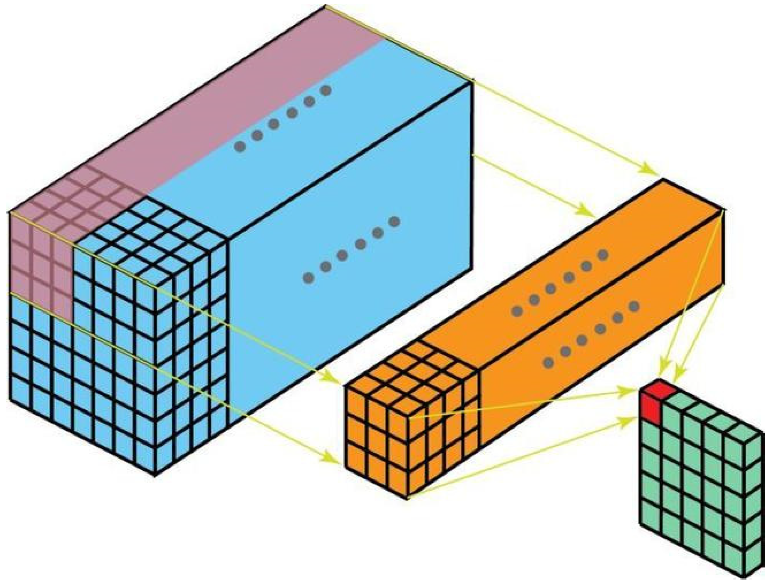
3.1. Three-Dimensional CNN
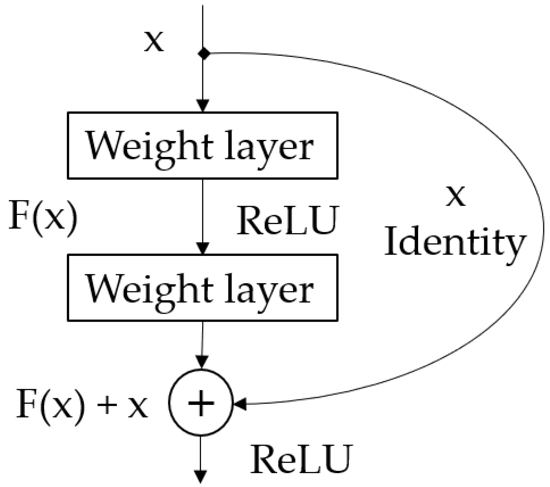
3.2. Residual Networks (ResNets)
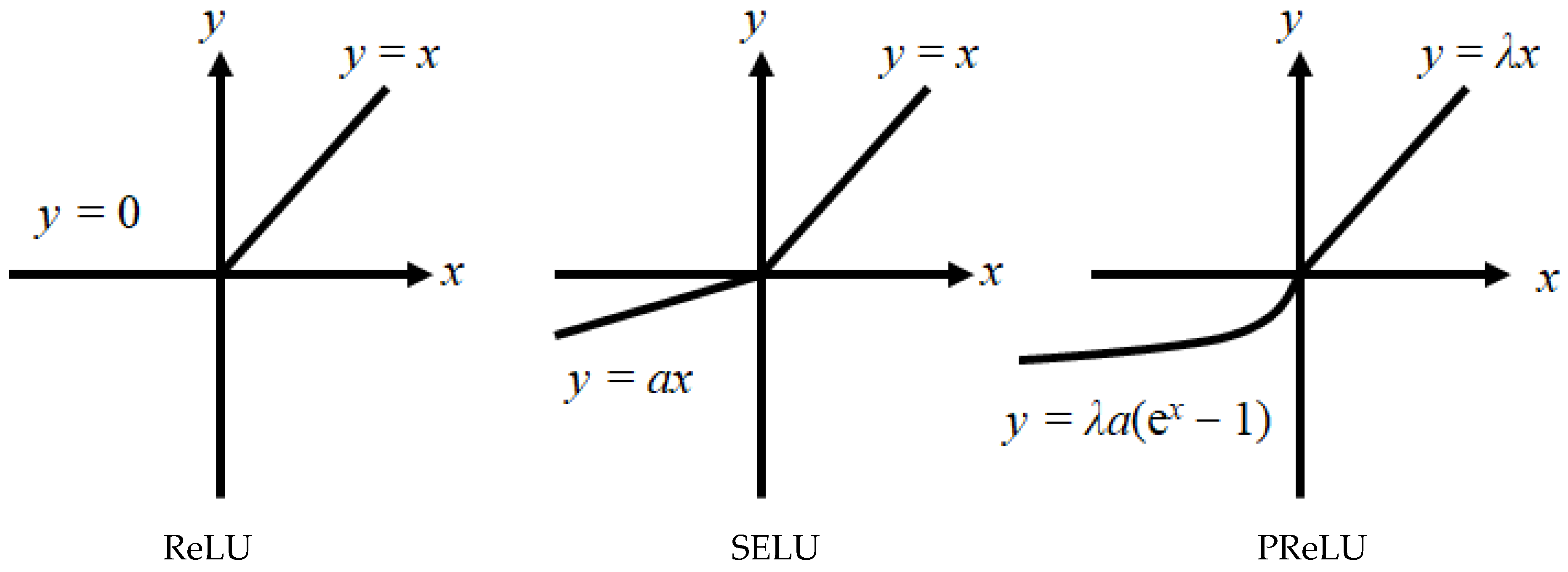
3.3. Activation Function
3.4. Loss Function
3.5. Multi-Shortcut-Link Networks (MSLNs)
3.5.1. Analysis of a Multi-Shortcut Link
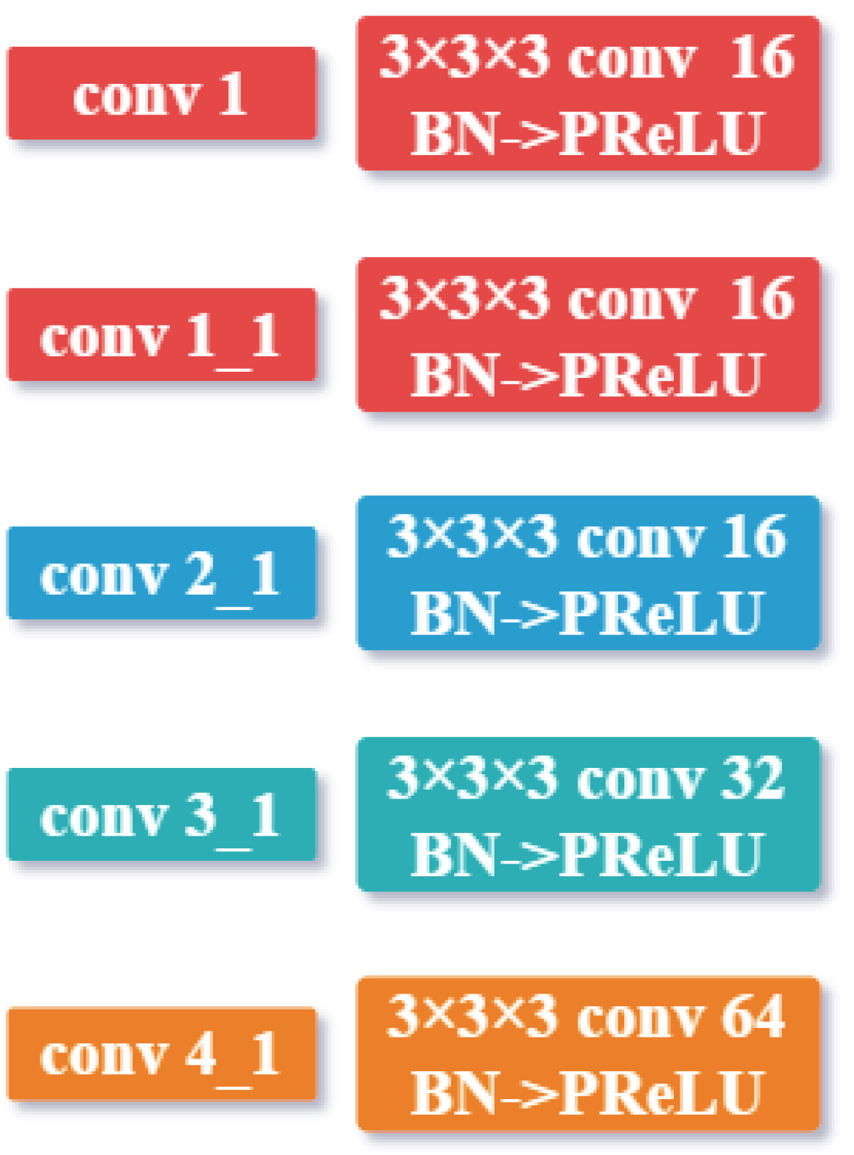
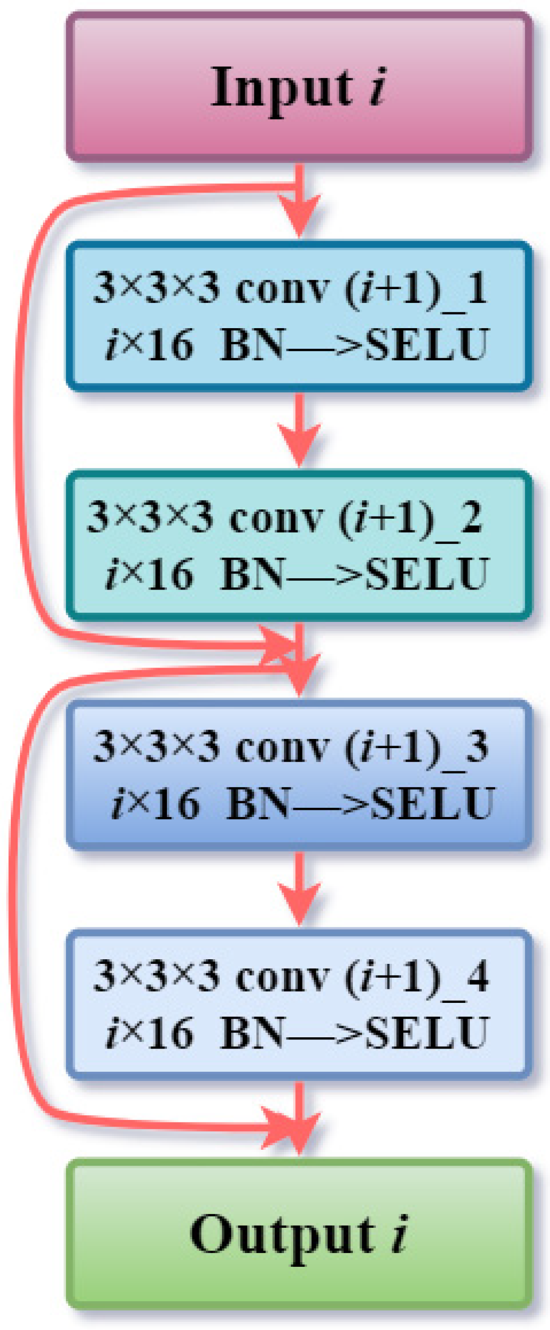
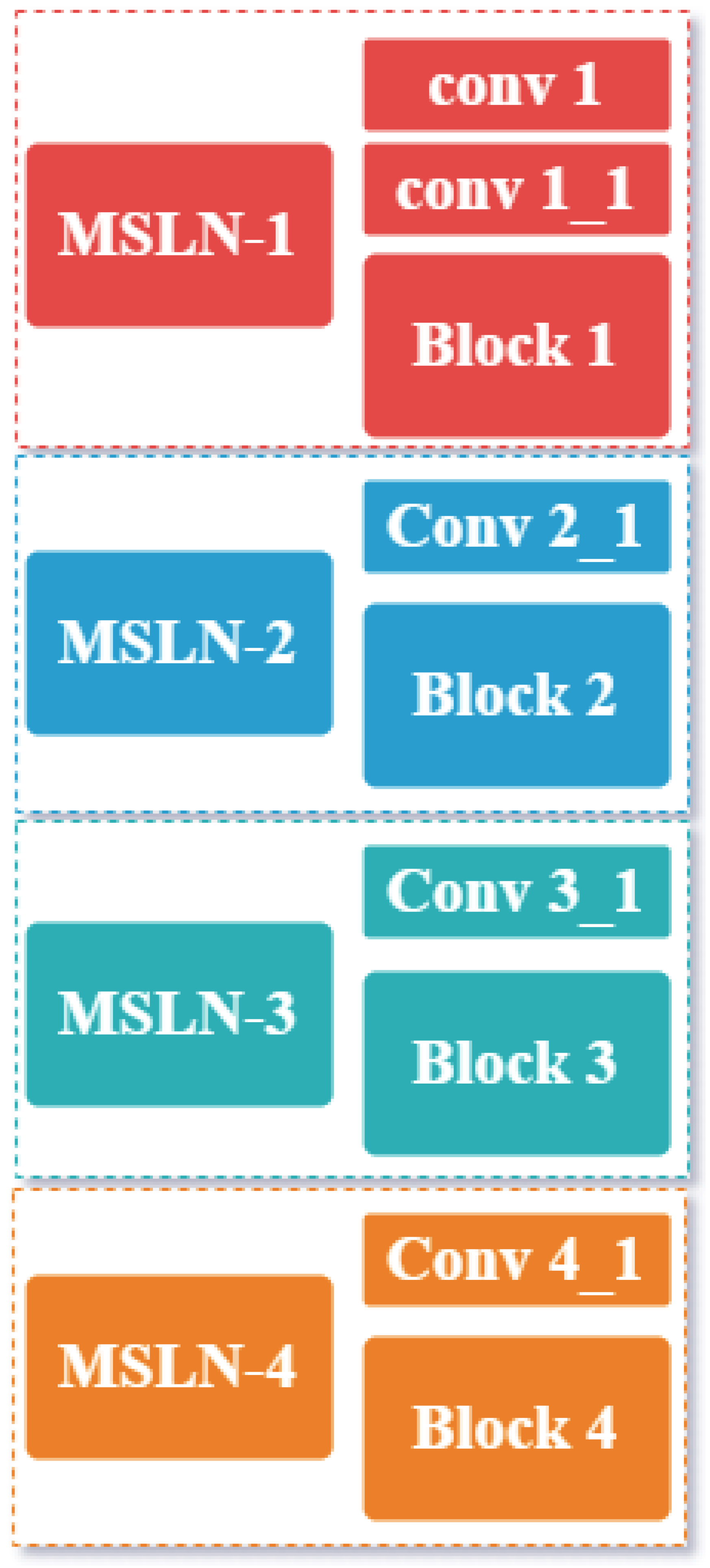
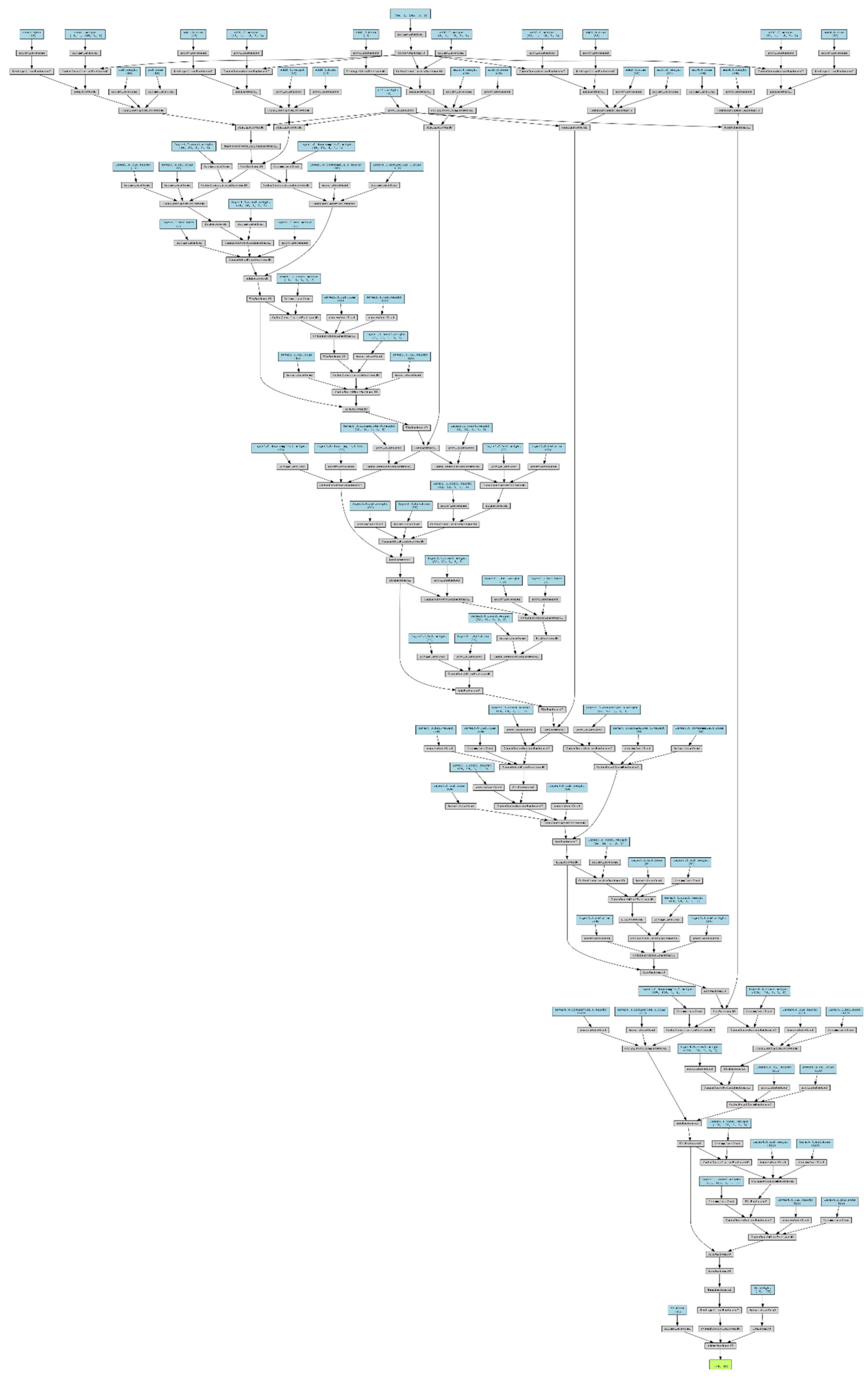
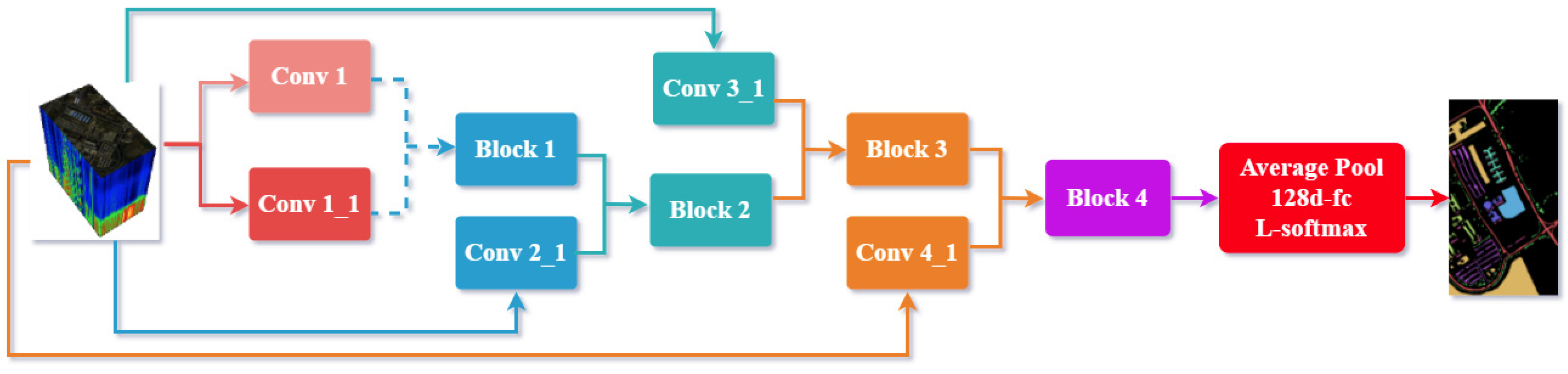
3.5.2. Structure of an MSLN
4. Datasets Results and Analysis
4.1. Hyperspectral Test Datasets
- (1)
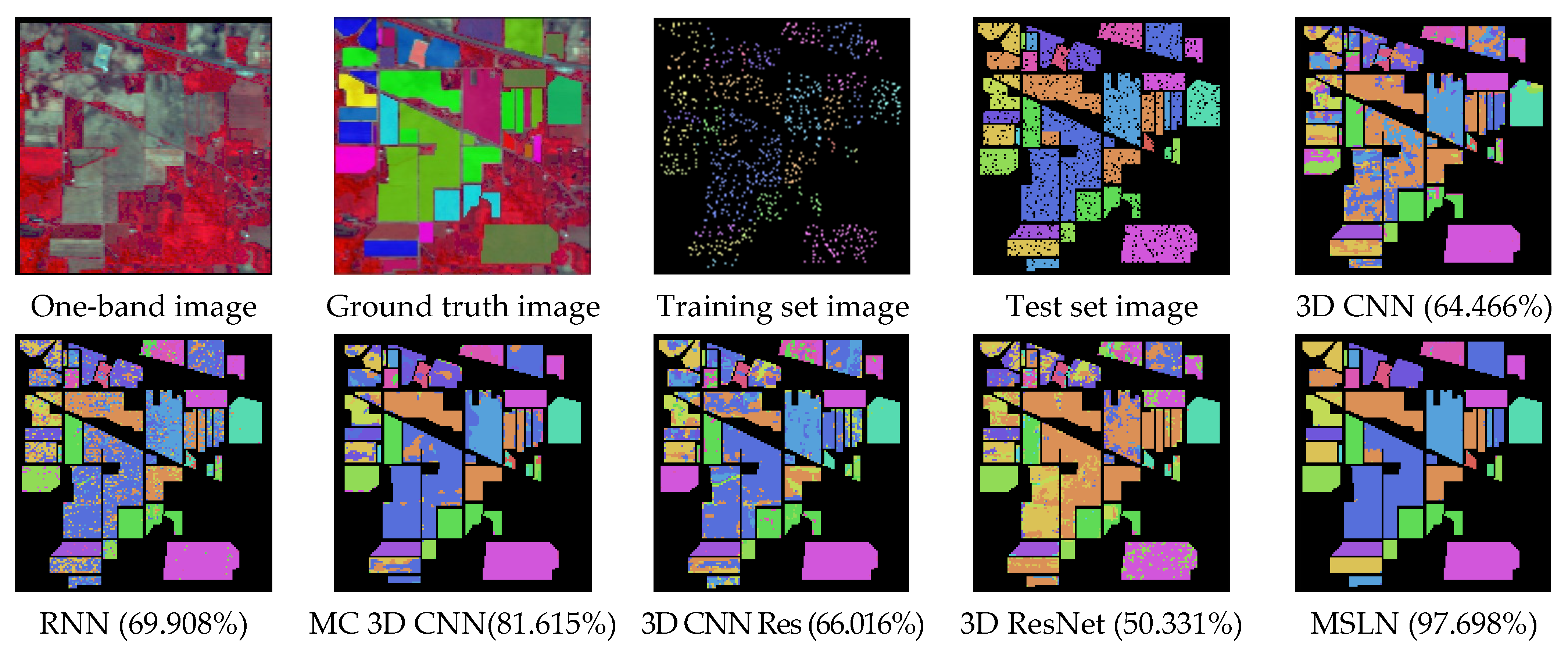
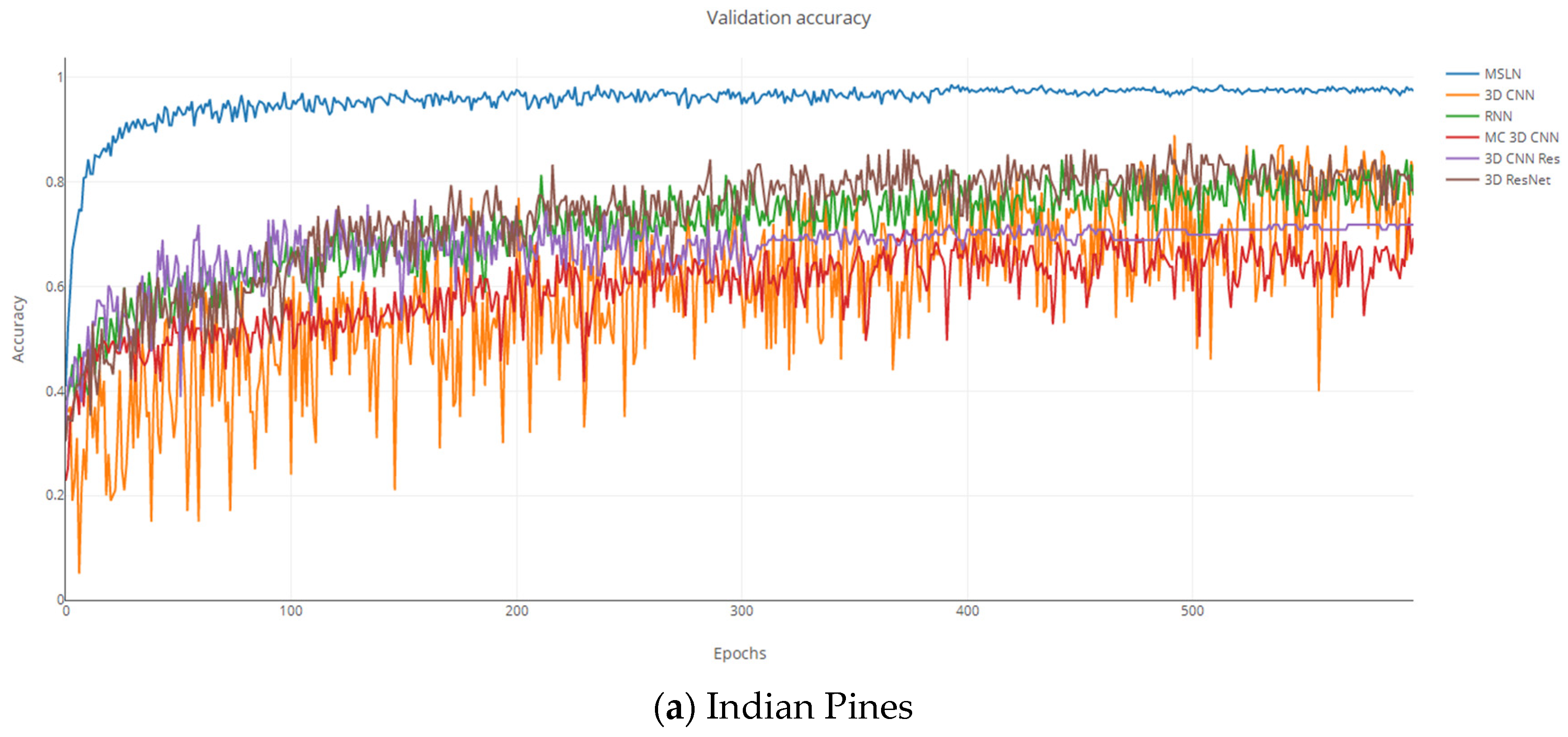
- Indian Pines (IP) Dataset
- (2)
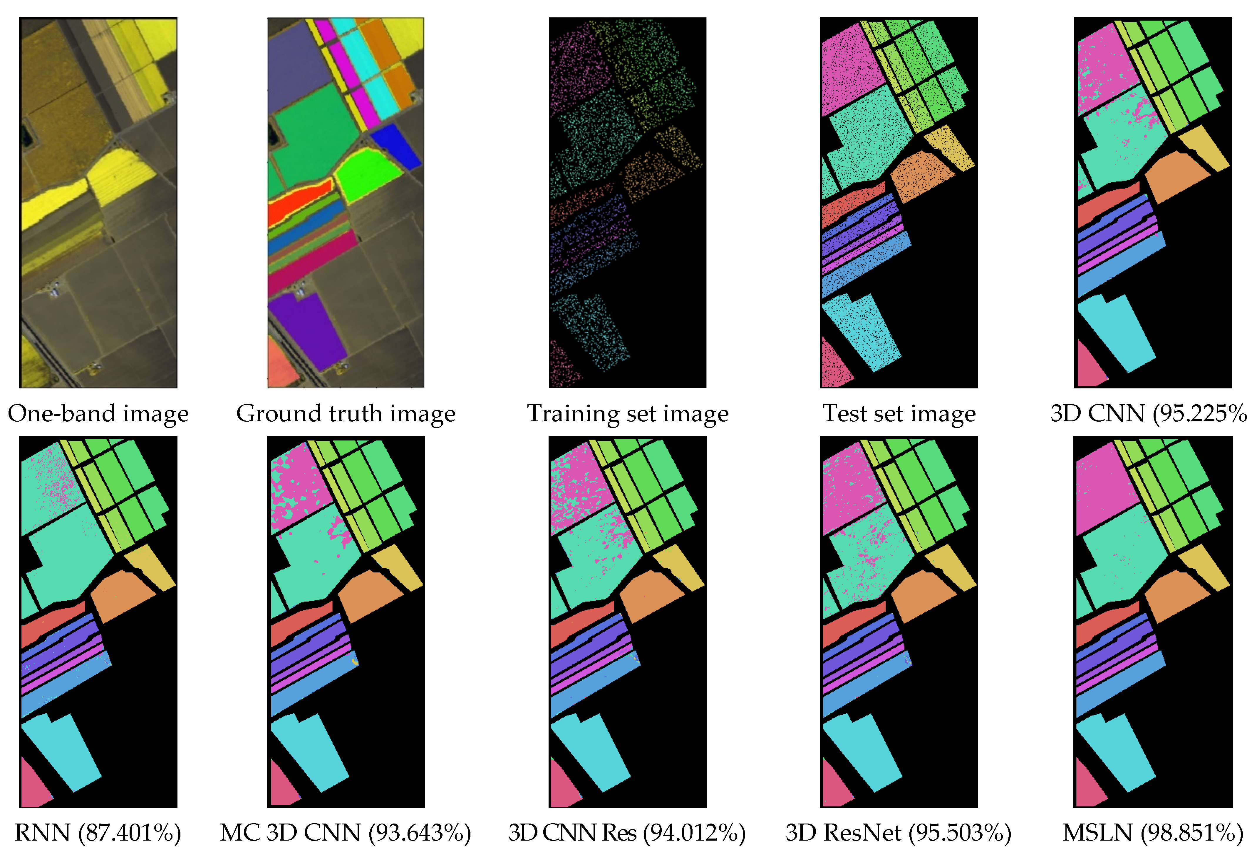
- Salinas (S) Dataset
- (3)
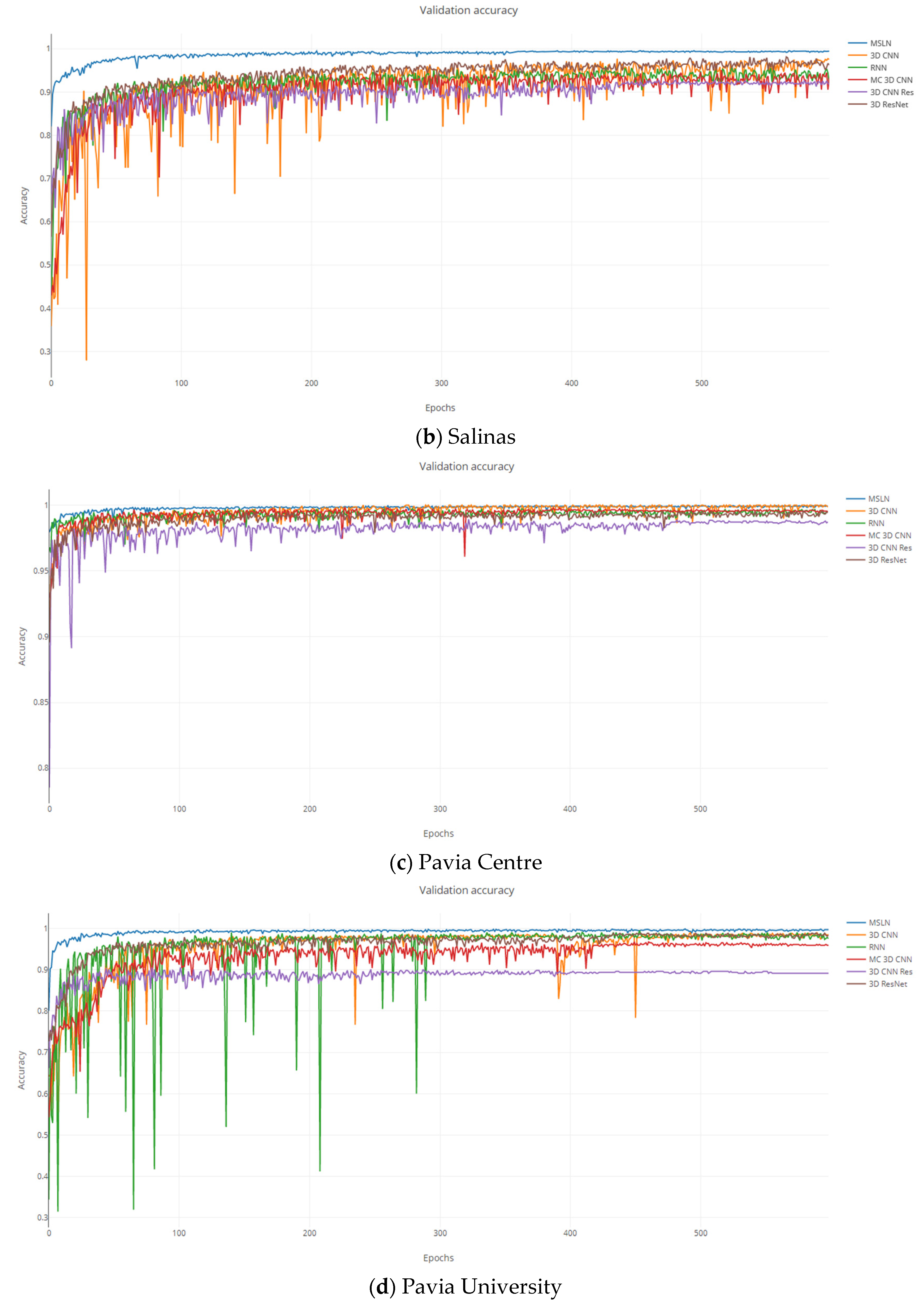
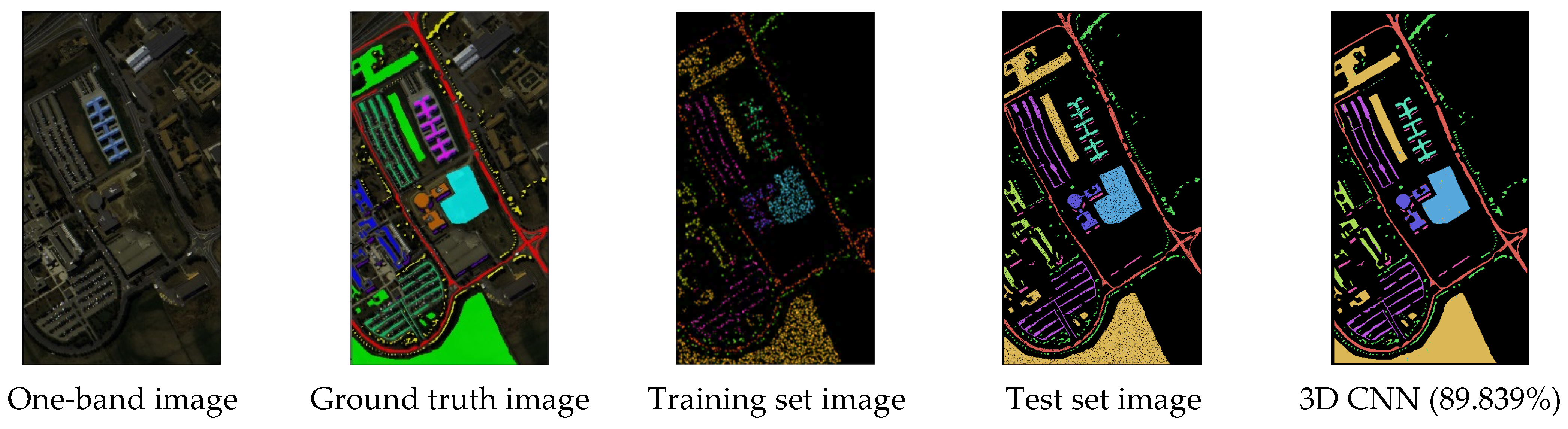
- Pavia Centre (PC) and Pavia University (PU) Datasets
- (4)
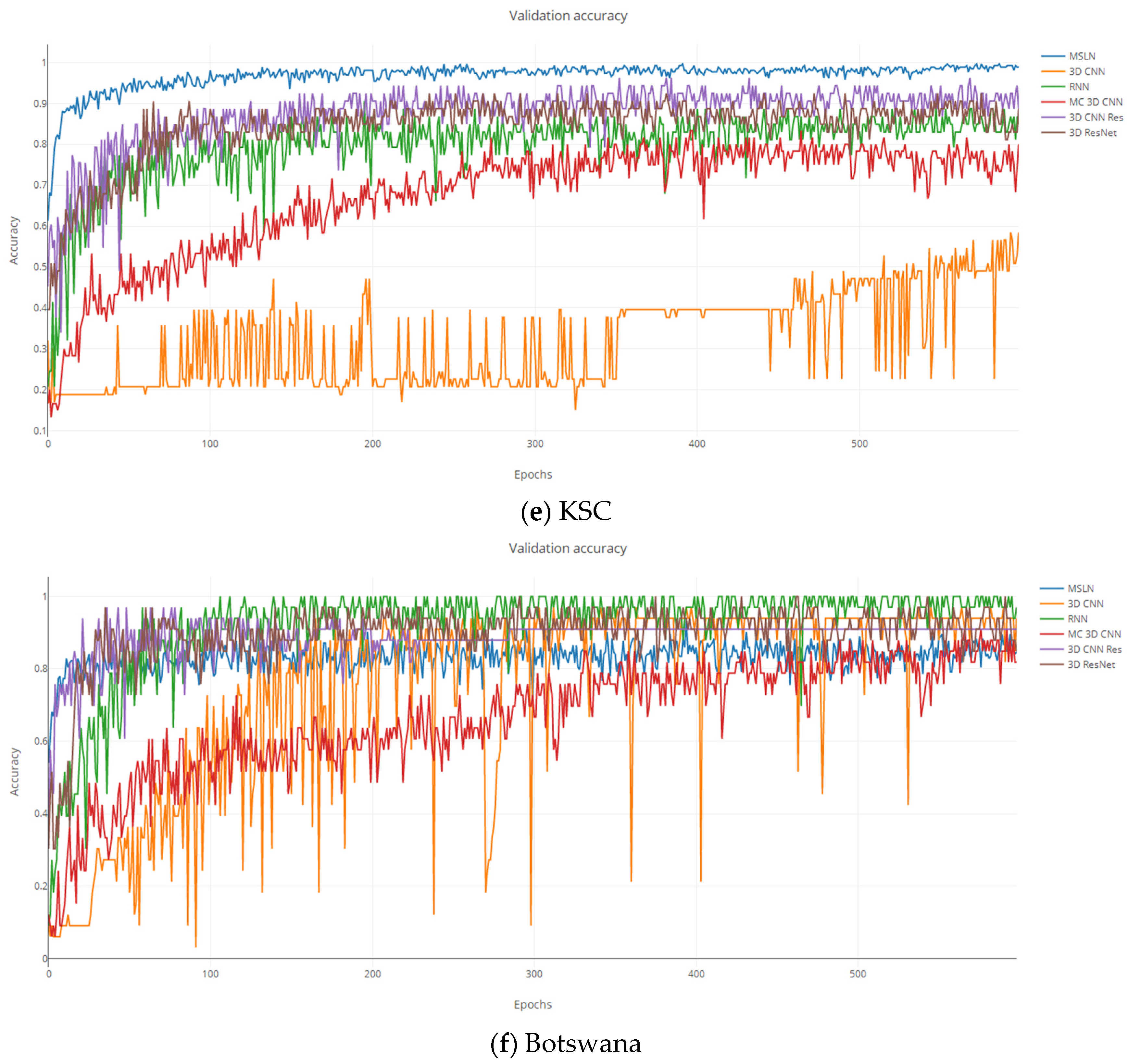
- Kennedy Space Center (KSC) Dataset
- (5)
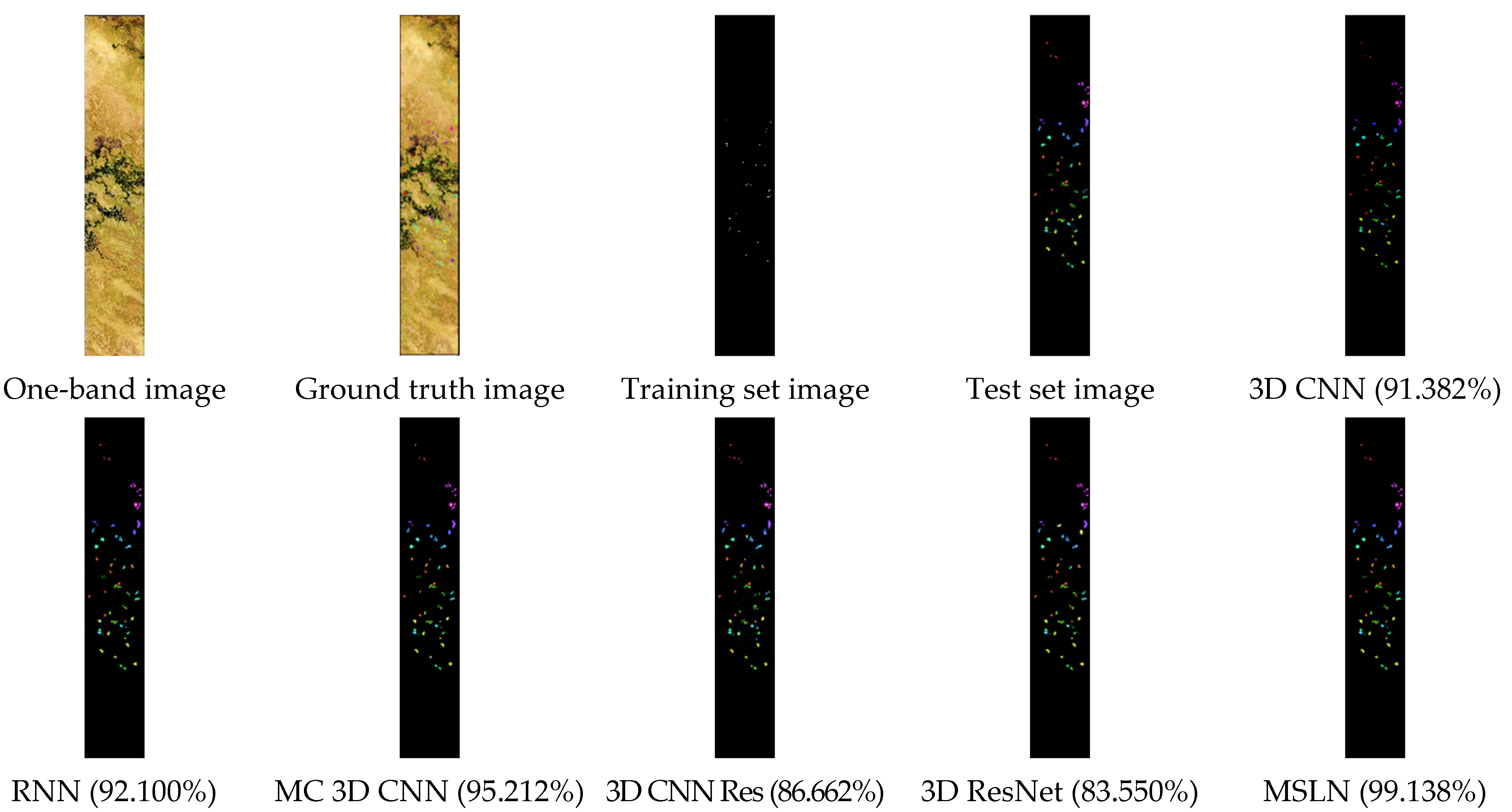
- Botswana (B) Dataset
4.2. Results and Analysis
5. Conclusions
Author Contributions
Funding
Institutional Review Board Statement
Informed Consent Statement
Conflicts of Interest
List of Acronyms
| HSI | Hyperspectral image |
| SVM | Support vector machine |
| ELM | Extreme learning machine |
| ANN | Artificial neural network |
| SAE | Stack autoencoding |
| DBN | Deep belief network |
| RNN | Recurrent neural network |
| CNN | Convolutional neural network |
| ResNet | Residual network |
| ResU | Residual unit |
| MSLN | Multi-shortcut-link network |
| ReLU | Rectified linear unit |
| SELU | Self-exponential linear unit |
| PReLU | Parametric rectified linear unit |
| MC 3D CNN | Multiscale 3D CNN |
| 3D CNN Res | 3D CNN residual |
| AA | Average accuracy |
| OA | Overall accuracy |
References
- Li, S.; Song, W.; Fang, L.; Chen, Y.; Ghamisi, P.; Benediktsson, J.A. Deep Learning for Hyperspectral Image Classification: An Overview. IEEE Trans. Geosci. Remote Sens. 2019, 57, 6690–6709. [Google Scholar] [CrossRef] [Green Version]
- Sun, L.; Wu, F.; He, C.; Zhan, T.; Liu, W.; Zhang, D. Weighted Collaborative Sparse and L1/2 Low-Rank Regularizations with Superpixel Segmentation for Hyperspectral Unmixing. IEEE Geosci. Remote Sens. Lett. 2020, 19, 1–5. [Google Scholar]
- Maes, W.H.; Steppe, K. Perspectives for remote sensing with unmanned aerial vehicles in precision agriculture. Trends Plant Sci. 2019, 24, 152–164. [Google Scholar] [CrossRef]
- Sun, H.; Zheng, X.; Lu, X.; Wu, S. Spectral-Spatial Attention Network for Hyperspectral Image Classification. IEEE Trans. Geosci. Remote Sens. 2019, 58, 3232–3245. [Google Scholar] [CrossRef]
- Shimoni, M.; Haelterman, R.; Perneel, C. Hypersectral Imaging for Military and Security Applications: Combining Myriad Processing and Sensing Techniques. IEEE Geosci. Remote Sens. Mag. 2019, 7, 101–117. [Google Scholar] [CrossRef]
- Yokoya, N.; Chan, J.C.; Segl, K. Potential of Resolution-Enhanced Hyperspectral Data for Mineral Mapping Using Simulated EnMAP and Sentinel-2 Images. Remote Sens. 2016, 8, 172. [Google Scholar] [CrossRef] [Green Version]
- Wu, H.; Lin, A.; Clarke, K.C.; Shi, W.; Cardenas-Tristan, A.; Tu, Z. A comprehensive quality assessment framework for linear features from Volunteered Geographic Information. Int. J. Geogr. Inf. Sci. 2021, 35, 1826–1847. [Google Scholar] [CrossRef]
- Lin, A.; Sun, X.; Wu, H.; Luo, W.; Wang, D.; Zhong, D.; Wang, Z.; Zhao, L.; Zhu, J. Identifying urban building function by integrating remote sensing imagery and POI data. IEEE J. Sel. Top. Appl. Earth Obs. Remote Sens. 2021, 14, 8864–8875. [Google Scholar] [CrossRef]
- Chehreghan, A.; Ali Abbaspour, R. An evaluation of data completeness of VGI through geometric similarity assessment. Int. J. Image Data Fusion 2018, 9, 319–337. [Google Scholar] [CrossRef]
- Barrington-Leigh, C.; Millard-Ball, A. The world’s user-generated road map is more than 80% complete. PLoS ONE 2017, 12, e0180698. [Google Scholar]
- Camps-Valls, G.; Bruzzone, L. Kernel-based methods for hyperspectral image classification. IEEE Trans. Geosci. Remote Sens. 2005, 43, 1351–1362. [Google Scholar] [CrossRef]
- Melgani, F.; Bruzzone, L. Classification of hyperspectral remote sensing images with support vector machines. IEEE Trans. Geosci. Remote Sens. 2004, 42, 1778–1790. [Google Scholar] [CrossRef] [Green Version]
- Huang, W.; Huang, Y.; Wang, H.; Liu, Y.; Shim, H.J. Local binary patterns and superpixel-based multiple kernels for hy-perspectral image classification. IEEE J. Sel. Top. Appl. Earth Obs. Remote Sens. 2020, 13, 4550–4563. [Google Scholar] [CrossRef]
- Ye, Q.; Zhao, H.; Li, Z.; Yang, X.; Gao, S.; Yin, T.; Ye, N. L1-Norm Distance Minimization-Based Fast Robust Twin Support Vector kk-Plane Clustering. IEEE Trans. Neural Netw. Learn. Syst. 2017, 29, 4494–4503. [Google Scholar] [CrossRef]
- Ghamisi, P.; Benediktsson, J.A.; Ulfarsson, M.O. Spectral-spatial hyperspectral image classification via multiscale adaptive sparse representation. IEEE Trans. Geosci. Remote Sens. 2014, 52, 2565–2574. [Google Scholar] [CrossRef] [Green Version]
- Liu, B.; Yu, X.; Zhang, P.; Tan, X.; Yu, A.; Xue, Z. semi-supervised convolutional neural network for hyperspectral image classification. Remote Sens. Lett. 2017, 8, 839–848. [Google Scholar] [CrossRef]
- Qin, A.; Shang, Z.; Tian, J.; Wang, Y.; Zhang, T.; Tang, Y.Y. Spectral-spatial Graph Convolutional Networks for Semisupervised Hyperspectral Image Classification. IEEE Geosci. Remote Sens. Lett. 2019, 16, 241–245. [Google Scholar] [CrossRef]
- Huang, G.B.; Ding, X.; Zhou, H. Optimization method based extreme learning machine for classification. Neurocomputing 2010, 74, 155–163. [Google Scholar] [CrossRef]
- Hernández-Espinosa, C.; Fernández-Redondo, M.; Torres-Sospedra, J. Some experiments with ensembles of neural networks for classification of hyperspectral images. In Proceedins of the International Symposium on Neural Networks, Dalian, China, 19–21 August 2004; Springer: Berlin/Heidelberg, Germany, 2004; pp. 912–917. [Google Scholar]
- Yu, C.; Xue, B.; Song, M.; Wang, Y.; Li, S.; Chang, C.I. Iterative Target-Constrained Interference-Minimized Classifier for Hyperspectral Classification. IEEE J. Sel. Top. Appl. Earth Obs. Remote Sens. 2018, 11, 1095–1117. [Google Scholar] [CrossRef]
- Luo, F.; Du, B.; Zhang, L.; Zhang, L.; Tao, D. Feature Learning Using Spatial-Spectral Hypergraph Discriminant Analysis for Hyperspectral Image. IEEE Trans. Cybern. 2019, 49, 2406–2419. [Google Scholar] [CrossRef]
- Yin, B.; Cui, B. Multi-feature extraction method based on Gaussian pyramid and weighted voting for hyperspectral image classification. In Proceedings of the 2021 IEEE International Conference on Consumer Electronics and Computer Engineering (ICCECE), Guangzhou, China, 15–17 January 2021; IEEE: New York, NY, USA, 2021; pp. 645–648. [Google Scholar]
- Huang, W.; Li, G.; Chen, Q.; Ju, M.; Qu, J. CF2PN: A Cross-Scale Feature Fusion Pyramid Network Based Remote Sensing Target Detection. Remote Sens. 2021, 13, 847. [Google Scholar] [CrossRef]
- Zhang, X.; Lu, W.; Li, F.; Peng, X.; Zhang, R. Deep Feature Fusion Model for Sentence Semantic Matching. Comput. Mater. Contin. 2019, 61, 601–616. [Google Scholar] [CrossRef]
- Wu, H.; Liu, Q.; Liu, X. A Review on Deep Learning Approaches to Image Classification and Object Segmentation. Comput. Mater. Contin. 2019, 60, 575–597. [Google Scholar] [CrossRef] [Green Version]
- Xu, Y.; Du, B.; Zhang, L. Beyond the Patchwise Classification: Spectral-spatial Fully Convolutional Networks for Hyperspectral Image Classification. IEEE Trans. Big Data 2020, 6, 492–506. [Google Scholar] [CrossRef]
- Jiang, Y.; Li, Y.; Zou, S.; Zhang, H.; Bai, Y. Hyperspectral Image Classification with Spatial Consistence Using Fully Convolutional Spatial Propagation Network. IEEE Trans. Geosci. Remote Sens. 2021, 59, 10425–10437. [Google Scholar] [CrossRef]
- Xu, Q.; Xiao, Y.; Wang, D.; Luo, B. CSA-MSO3DCNN: Multiscale Octave 3D CNN with Channel and Spatial Attention for Hyperspectral Image Classification. Remote Sens. 2020, 12, 188. [Google Scholar] [CrossRef] [Green Version]
- Chen, Y.; Lin, Z.; Zhao, X.; Wang, G.; Gu, Y. Deep Learning-Based Classification of Hyperspectral Data. IEEE J. Sel. Top. Appl. Earth Obs. Remote Sens. 2017, 7, 2094–2107. [Google Scholar]
- Suk, H.-I.; Lee, S.-W.; Shen, D. Latent feature representation with stacked auto-encoder for AD/MCI diagnosis. Brain Struct. Funct. 2015, 220, 841–859. [Google Scholar] [CrossRef]
- Chen, Y.; Zhao, X.; Jia, X. Spectral-Spatial Classification of Hyperspectral Data Based on Deep Belief Network. IEEE J. Sel. Top. Appl. Earth Obs. Remote Sens. 2015, 8, 2381–2392. [Google Scholar] [CrossRef]
- Mou, L.; Ghamisi, P.; Zhu, X.X. Deep Recurrent Neural Networks for Hyperspectral Image Classification. IEEE Trans. Geosci. Remote Sens. 2017, 55, 3639–3655. [Google Scholar] [CrossRef] [Green Version]
- Seydgar, M.; Alizadeh Naeini, A.; Zhang, M.; Li, W.; Satari, M. 3-D convolution-recurrent networks for spectral-spatial clas-sification of hyperspectral images. Remote Sens. 2019, 11, 883. [Google Scholar] [CrossRef] [Green Version]
- He, C.; Sun, L.; Huang, W.; Zhang, J.; Zheng, Y.; Jeon, B. TSLRLN: Tensor subspace low-rank learning with non-local prior for hyperspectral image mixed denoising. Signal Process. 2021, 184, 108060. [Google Scholar] [CrossRef]
- Sharma, V.; Diba, A.; Tuytelaars, T.; Van Gool, L. Hyperspectral CNN for Image Classification & Band Selection, with Application to Face Recognition; Technical Report: KUL/ESAT/PSI/1604; KU Leuven, ESAT: Leuven, Belgium, 2016. [Google Scholar]
- Hu, W.; Huang, Y.; Wei, L.; Zhang, F.; Li, H. Deep Convolutional Neural Networks for Hyperspectral Image Classification. J. Sens. 2015, 2015, 258619. [Google Scholar] [CrossRef] [Green Version]
- Hamida, A.B.; Benoit, A.; Lambert, P.; Amar, C.B. 3-D Deep Learning Approach for Remote Sensing Image Classification. IEEE Trans. Geosci. Remote Sens. 2018, 56, 4420–4434. [Google Scholar] [CrossRef] [Green Version]
- Chen, Y.; Jiang, H.; Li, C.; Jia, X.; Ghamisi, P. Deep Feature Extraction and Classification of Hyperspectral Images Based on Convolutional Neural Networks. IEEE Trans. Geosci. Remote Sens. 2016, 54, 6232–6251. [Google Scholar] [CrossRef] [Green Version]
- Ying, L.; Haokui, Z.; Qiang, S. Spectral–Spatial Classification of Hyperspectral Imagery with 3D Convolutional Neural Network. Remote Sens. 2017, 9, 67. [Google Scholar]
- Luo, Y.; Zou, J.; Yao, C.; Zhao, X.; Li, T.; Bai, G. HSI-CNN: A Novel Convolution Neural Network for Hyperspectral Image. In Proceedins of the 2018 International Conference on Audio, Language and Image Processing (ICALIP), Shanghai, China, 16–17 July 2018; IEEE: New York, NY, USA, 2018. [Google Scholar]
- Lee, H.; Kwon, H. Contextual Deep CNN Based Hyperspectral Classification. In Proceedings of the Geoscience & Remote Sensing Symposium, Beijing, China, 10–15 July 2016; IEEE: New York, NY, USA, 2016; pp. 3322–3325. [Google Scholar]
- He, M.; Li, B.; Chen, H. Multi-scale 3D deep convolutional neural network for hyperspectral image classification. In Proceedings of the 2017 IEEE International Conference on Image Processing (ICIP), Beijing, China, 17–20 September2017; IEEE: New York, NY, USA, 2017; pp. 3904–3908. [Google Scholar]
- Sun, L.; He, C.; Zheng, Y.; Tang, S. SLRL4D: Joint restoration of subspace low-rank learning and non-local 4-D transform filtering for hyperspectral image. Remote Sens. 2020, 12, 2979. [Google Scholar] [CrossRef]
- Gao, H.; Chen, Z.; Li, C. Sandwich Convolutional Neural Network for Hyperspectral Image Classification Using Spectral Feature Enhancement. IEEE J. Sel. Top. Appl. Earth Obs. Remote Sens. 2021, 14, 3006–3015. [Google Scholar] [CrossRef]
- Bishop, C.M. Neural Networks for Pattern Recognition; Oxford University Press: Oxford, UK, 1995. [Google Scholar]
- Ripley, B.D. Pattern Recognition and Neural Networks; Cambridge University Press: Cambridge, UK, 2007. [Google Scholar]
- Venables, W.N.; Ripley, B.D. Modern Applied Statistics with S-PLUS; Springer Science & Business Media: Berlin/Heidelberg, Germany, 2013. [Google Scholar]
- Szegedy, C.; Liu, W.; Jia, Y.; Sermanet, P.; Reed, S.; Anguelov, R.; Erhan, D.; Vanhoucke, V.; Rabinovich, A. Going deeper with convolutions. In Proceedings of the IEEE Conference on Computer Vision and Pattern Recognition, Boston, MA, USA, 17–20 June 2015; pp. 1–9. [Google Scholar]
- Lee, C.Y.; Xie, S.; Gallagher, P.; Zhang, Z.; Tu, Z. Deeply-supervised nets. In Proceedings of the Artificial Intelligence and Statistics, San Diego, California, USA, 9–12 May 2015; PMLR: New York, NY, USA, 2015; pp. 562–570. [Google Scholar]
- Raiko, T.; Valpola, H.; LeCun, Y. Deep learning made easier by linear transformations in perceptrons. In Proceedings of the Artificial intelligence and statistics, La Palma, Canary Islands, 21–23 April 2012; PMLR: New York, NY, USA, 2012; pp. 924–932. [Google Scholar]
- Schraudolph, N. Accelerated Gradient Descent by Factor-Centering Decomposition; Technical report/IDSIA; IDSIA: Lugano, Switzerland, 1998; p. 98. [Google Scholar]
- Schraudolph, N.N. Centering neural network gradient factors. In Neural Networks: Tricks of the Trade; Springer: Berlin/Heidelberg, Germany, 1998; pp. 207–226. [Google Scholar]
- Vatanen, T.; Raiko, T.; Valpola, H.; LeCun, Y. Pushing stochastic gradient towards second-order methods–backpropagation learning with transformations in nonlinearities. In Proceedings of the International Conference on Neural Information Processing, Daegu, Korea, 3–7 November 2013; Springer: Berlin/Heidelberg, Germany, 2013; pp. 442–449. [Google Scholar]
- Ioffe, S.; Szegedy, C. Batch normalization: Accelerating deep network training by reducing internal covariate shift. In Proceedings of the International Conference on Machine Learning, Lille, France, 6–11 July 2015; PMLR: New York, NY, USA, 2015; pp. 448–456. [Google Scholar]
- Szegedy, C.; Vanhoucke, V.; Ioffe, S.; Shlens, J.; Wojna, Z. Rethinking the inception architecture for computer vision. In Proceedings of the IEEE Conference on Computer Vision and Pattern Recognition, Las Vegas, NV, USA, 27–30 June 2016; pp. 2818–2826. [Google Scholar]
- He, K.; Zhang, X.; Ren, S.; Sun, J. Deep residual learning for image recognition. In Proceedings of the IEEE Conference on Computer Vision and Pattern Recognition, Las Vegas, NV, USA, 27–30 June 2016; pp. 770–778. [Google Scholar]
- He, K.; Zhang, X.; Ren, S.; Sun, J. Identity mappings in deep residual networks. In Proceedings of the European Conference on Computer Vision, Amsterdam, The Netherlands, 8–16 October 2016; Springer: Cham, Switzerland, 2016; pp. 630–645. [Google Scholar]
- Szegedy, C.; Ioffe, S.; Vanhoucke, V.; Alemi, A.A. Inception-v4, inception-resnet and the impact of residual connections on learning. In Proceedings of the thirty-first AAAI Conference on Artificial Intelligence, San Francisco, CA, USA, 4–9 February 2017; pp. 4278–4284. [Google Scholar]
- Lu, Y.S.; Li, Y.X.; Liu, B. Hyperspectral Data Haze Monitoring Based on Deep Residual Network. Acta Opt. Sin. 2017, 37, 1128001. [Google Scholar]
- Liu, D.; Han, G.; Liu, P.; Yang, H.; Sun, X.; Li, Q.; Wu, J. A Novel 2D-3D CNN with Spectral-Spatial Multi-Scale Feature Fusion for Hyperspectral Image Classification. Remote Sens. 2021, 13, 4621. [Google Scholar] [CrossRef]
- Meng, Z.; Jiao, L.; Liang, M.; Zhao, F. Hyperspectral Image Classification with Mixed Link Networks. IEEE J. Sel. Top. Appl. Earth Obs. Remote Sens. 2021, 14, 2494–2507. [Google Scholar] [CrossRef]
- Zhong, Z.; Li, J.; Luo, Z.; Chapman, M. Spectral-spatial Residual Network for Hyperspectral Image Classification: A 3-D Deep Learning Framework. IEEE Trans. Geosci. Remote Sens. 2018, 56, 847–858. [Google Scholar] [CrossRef]
- Cao, F.; Guo, W. Deep hybrid dilated residual networks for hyperspectral image classification. Neurocomputing 2020, 384, 170–181. [Google Scholar] [CrossRef]
- Xu, Y.; Li, Z.; Li, W.; Du, Q.; Liu, C.; Fang, Z.; Zhai, L. Dual-channel residual network for hyperspectral image classification with noisy labels. IEEE Trans. Geosci. Remote Sens. 2021, 60, 1–11. [Google Scholar] [CrossRef]
- Gao, H.; Yang, Y.; Li, C.; Gao, L.; Zhang, B. Multiscale residual network with mixed depthwise convolution for hyperspectral image classification. IEEE Trans. Geosci. Remote Sens. 2021, 59, 3396–3408. [Google Scholar] [CrossRef]
- Dang, L.; Pang, P.; Lee, J. Depth-Wise Separable Convolution Neural Network with Residual Connection for Hyperspectral Image Classification. Remote Sens. 2020, 12, 3408. [Google Scholar] [CrossRef]
- Paoletti, M.E.; Haut, J.M.; Fernandez-Beltran, R.; Plaza, J.; Plaza, A.J.; Pla, F. Deep pyramidal residual networks for spectral–spatial hyperspectral image classification. IEEE Trans. Geosci. Remote Sens. 2019, 57, 740–754. [Google Scholar] [CrossRef]
- Wang, L.; Peng, J.; Sun, W. Spatial–spectral squeeze-and-excitation residual network for hyperspectral image classification. Remote Sens. 2019, 11, 884. [Google Scholar] [CrossRef] [Green Version]
- Zhang, X.; Wang, Y.; Zhang, N.; Xu, D.; Luo, H.; Chen, B.; Ben, G. Spectral-spatial Fractal Residual Convolutional Neural Network with Data Balance Augmentation for Hyperspectral Classification. IEEE Trans. Geosci. Remote Sens. 2021, 59, 10473–10487. [Google Scholar] [CrossRef]
- Xu, H.; Yao, W.; Cheng, L.; Li, B. Multiple Spectral Resolution 3D Convolutional Neural Network for Hyperspectral Image Classification. Remote Sens. 2021, 13, 1248. [Google Scholar] [CrossRef]
- Glorot, X.; Bordes, A.; Bengio, Y. Deep sparse rectifier neural networks. In Proceedings of the Fourteenth International Conference on Artificial Intelligence and Statistics, Fort Lauderdale, FL, USA, 11–13 April 2011; pp. 315–323. [Google Scholar]
- He, K.; Zhang, X.; Ren, S.; Sun, J. Delving deep into rectifiers: Surpassing human-level performance on imagenet classification. In Proceedings of the IEEE International Conference on Computer Vision, Santiago, Chile, 7–13 December 2015; pp. 1026–1034. [Google Scholar]
- Klambauer, G.; Unterthiner, T.; Mayr, A.; Hochreiter, S. Self-normalizing neural networks. In Proceedings of the 31st international conference on neural information processing systems, Long Beach, CA, USA, 4–9 December 2017; pp. 972–981. [Google Scholar]
- Liu, W.; Wen, Y.; Yu, Z.; Yang, M. Large-Margin Softmax Loss for Convolutional Neural Networks. In Proceedings of the 33rd International Conference on Machine Learning, New York, NY, USA, 19–24 June 2016; pp. 507–516. [Google Scholar]
- Zhang, Y.Z.; Xu, M.M.; Wang, X.H.; Wang, K.Q. Hyperspectral image classification based on hierarchical fusion of residual networks. Spectrosc. Spectr. Anal. 2019, 39, 3501–3507. [Google Scholar]
- Graña, M.; Veganzons, M.A.; Ayerdi, B. Hyperspectral Remote Sensing Scenes. Available online: http://www.ehu.eus/ccwintco/index.php?title=Hyperspectral_Remote_Sensing_Scenes (accessed on 6 October 2021).


| Layer_Name | 18-Layer ResNet Kernel_Size Kernel_Number Stride | Layer_Name | 22-Layer MSLN Kernel_Size Kernel_Number Stride |
|---|---|---|---|
| conv 1 | conv 1 | ||
| conv 1_1 | |||
| Block1 | Block1 | ||
| Block2 | conv 2_1 | ||
| Block2 | |||
| Block3 | conv 3_1 | ||
| Block3 | |||
| Block4 | conv 4_1 | ||
| Block4 | |||
| Average pool 1000-d fc l-softmax | Average pool 128-d fc l-softmax | ||
| Sample No. | Class | Train | Validation | Test |
|---|---|---|---|---|
| 1 | Alfalfa | 4 | 1 | 41 |
| 2 | Corn-notill | 129 | 14 | 1285 |
| 3 | Corn-mintill | 75 | 8 | 747 |
| 4 | Corn | 22 | 2 | 213 |
| 5 | Grass-pasture | 43 | 5 | 435 |
| 6 | Grass-trees | 43 | 7 | 680 |
| 7 | Grass-pasture-mowed | 3 | 1 | 24 |
| 8 | Hay-windrowed | 43 | 5 | 430 |
| 9 | Oats | 3 | 1 | 16 |
| 10 | Soybean-notill | 87 | 10 | 875 |
| 11 | Soybean-mintill | 220 | 25 | 2210 |
| 12 | Soybean-clean | 53 | 6 | 534 |
| 13 | Wheat | 18 | 2 | 185 |
| 14 | Woods | 113 | 13 | 1139 |
| 15 | Buildings-grass-trees-drives | 35 | 4 | 347 |
| 16 | Stone-steel-towers | 8 | 1 | 84 |
| Total | 899 | 105 | 9245 |
| Sample No. | Class | Train | Validation | Test |
|---|---|---|---|---|
| 1 | Brocoli_green_weeds_1 | 181 | 20 | 1808 |
| 2 | Brocoli_green_weeds_2 | 355 | 37 | 3334 |
| 3 | Fallow | 177 | 20 | 1779 |
| 4 | Fallow_rough_plow | 125 | 14 | 1255 |
| 5 | Fallow_smooth | 241 | 27 | 2410 |
| 6 | Stubble | 357 | 39 | 3563 |
| 7 | Celery | 322 | 36 | 3221 |
| 8 | Grapes_untrained | 1014 | 113 | 10,144 |
| 9 | Soil_vinyard_develop | 558 | 62 | 5583 |
| 10 | Corn_senesced_green_weeds | 292 | 33 | 2953 |
| 11 | Lettuce_romaine_4wk | 96 | 11 | 961 |
| 12 | Lettuce_romaine_5wk | 171 | 19 | 1737 |
| 13 | Lettuce_romaine_6wk | 81 | 9 | 826 |
| 14 | Lettuce_romaine_7wk | 96 | 11 | 963 |
| 15 | Vineyard_untrained | 646 | 71 | 6551 |
| 16 | Vineyard_vertical_trellis | 157 | 17 | 1633 |
| Total | 4869 | 539 | 48,721 |
| Sample No. | Class | Train | Validation | Test |
|---|---|---|---|---|
| 1 | Water | 5925 | 657 | 59,251 |
| 2 | Trees | 684 | 76 | 6838 |
| 3 | Asphalt | 277 | 31 | 2736 |
| 4 | Self-blocking bricks | 241 | 27 | 2417 |
| 5 | Bitumen | 592 | 66 | 5924 |
| 6 | Tiles | 833 | 92 | 8317 |
| 7 | Shadows | 656 | 73 | 6558 |
| 8 | Meadows | 3842 | 425 | 38,415 |
| 9 | Bare soil | 257 | 29 | 2577 |
| Total | 13,307 | 1476 | 133,033 |
| Sample No. | Class | Train | Validation | Test |
|---|---|---|---|---|
| 1 | Asphalt | 593 | 65 | 5973 |
| 2 | Meadows | 1674 | 186 | 16,789 |
| 3 | Gravel | 188 | 21 | 1890 |
| 4 | Trees | 275 | 31 | 2758 |
| 5 | Painted metal sheets | 121 | 13 | 1211 |
| 6 | Bare Soil | 453 | 50 | 4526 |
| 7 | Bitumen | 120 | 13 | 1197 |
| 8 | Self-blocking bricks | 331 | 37 | 3314 |
| 9 | Shadows | 85 | 10 | 852 |
| Total | 3840 | 426 | 38,510 |
| Sample No. | Class | Train | Validation | Test |
|---|---|---|---|---|
| 1 | Scrub | 68 | 8 | 685 |
| 2 | Willow-swamp | 22 | 2 | 219 |
| 3 | Cabbage palm hammock | 23 | 3 | 230 |
| 4 | Cabbage palm/oak hammock | 22 | 3 | 227 |
| 5 | Slash pine | 14 | 2 | 145 |
| 6 | Oak/broadleaf hammock | 21 | 2 | 206 |
| 7 | Hardwood swamp | 10 | 1 | 94 |
| 8 | Graminoid marsh | 39 | 4 | 388 |
| 9 | Spartina marsh | 47 | 5 | 468 |
| 10 | Cattail marsh | 36 | 4 | 364 |
| 11 | Salt marsh | 38 | 4 | 377 |
| 12 | Mud flats | 45 | 5 | 453 |
| 13 | Wate | 83 | 10 | 834 |
| Total | 468 | 53 | 4690 |
| Sample No. | Class | Train | Validation | Test |
|---|---|---|---|---|
| 1 | Water | 24 | 3 | 243 |
| 2 | Hippo grass | 9 | 1 | 91 |
| 3 | Floodplain grasses 1 | 23 | 2 | 226 |
| 4 | Floodplain grasses 2 | 19 | 2 | 194 |
| 5 | Reeds | 24 | 3 | 242 |
| 6 | Riparian | 24 | 3 | 242 |
| 7 | Firescar | 23 | 3 | 233 |
| 8 | Island interior | 18 | 2 | 183 |
| 9 | Acacia woodlands | 28 | 3 | 283 |
| 10 | Acacia shrublands | 23 | 2 | 233 |
| 11 | Acacia grasslands | 27 | 3 | 275 |
| 12 | Short mopane | 16 | 2 | 163 |
| 13 | Mixed mopane | 24 | 3 | 241 |
| 14 | Exposed soils | 9 | 1 | 85 |
| Total | 291 | 33 | 2934 |
| Indian Pines | 3D CNN | RNN | MC 3D CNN | 3D CNN Res | 3D ResNet | MSLN |
|---|---|---|---|---|---|---|
| 1 | 0.656 | 0.436 | 0.543 | 0.000 | 0.086 | 0.978 |
| 2 | 0.563 | 0.646 | 0.815 | 0.454 | 0.491 | 0.982 |
| 3 | 0.626 | 0.424 | 0.591 | 0.555 | 0.313 | 0.961 |
| 4 | 0.543 | 0.362 | 0.825 | 0.416 | 0.269 | 0.947 |
| 5 | 0.710 | 0.821 | 0.868 | 0.361 | 0.664 | 0.996 |
| 6 | 0.916 | 0.894 | 0.969 | 0.857 | 0.878 | 0.995 |
| 7 | 0.864 | 0.323 | 0.700 | 0.343 | 0.077 | 1.000 |
| 8 | 0.907 | 0.939 | 0.968 | 0.939 | 0.912 | 0.996 |
| 9 | 0.000 | 0.538 | 0.944 | 0.000 | 0.329 | 1.000 |
| 10 | 0.586 | 0.566 | 0.762 | 0.640 | 0.068 | 0.979 |
| 11 | 0.433 | 0.670 | 0.808 | 0.709 | 0.175 | 0.986 |
| 12 | 0.535 | 0.599 | 0.731 | 0.339 | 0.500 | 0.981 |
| 13 | 0.952 | 0.956 | 1.000 | 0.921 | 0.930 | 1.000 |
| 14 | 0.924 | 0.928 | 0.952 | 0.843 | 0.847 | 0.987 |
| 15 | 0.582 | 0.575 | 0.665 | 0.532 | 0.429 | 0.912 |
| 16 | 0.794 | 0.852 | 0.903 | 0.839 | 0.880 | 0.989 |
| Kappa | 0.601 | 0.655 | 0.789 | 0.610 | 0.449 | 0.974 |
| AA | 0.662 | 0.658 | 0.815 | 0.547 | 0.491 | 0.981 |
| OA (%) | 64.466 | 69.908 | 81.615 | 66.016 | 50.331 | 97.698 |
| Salinas | 3D CNN | RNN | MC 3D CNN | 3D CNN Res | 3D ResNet | MSLN |
|---|---|---|---|---|---|---|
| 1 | 0.983 | 0.997 | 0.976 | 0.995 | 0.991 | 0.993 |
| 2 | 1.000 | 0.998 | 0.999 | 0.995 | 1.000 | 1.000 |
| 3 | 0.997 | 0.983 | 0.988 | 0.985 | 0.995 | 1.000 |
| 4 | 0.997 | 0.988 | 0.992 | 0.996 | 0.996 | 0.999 |
| 5 | 0.996 | 0.981 | 0.996 | 0.989 | 0.994 | 1.000 |
| 6 | 0.996 | 0.999 | 0.992 | 0.999 | 1.000 | 1.000 |
| 7 | 0.993 | 0.998 | 0.993 | 0.996 | 0.998 | 1.000 |
| 8 | 0.920 | 0.778 | 0.905 | 0.878 | 0.911 | 0.985 |
| 9 | 0.997 | 0.987 | 0.996 | 0.997 | 0.998 | 1.000 |
| 10 | 0.977 | 0.963 | 0.955 | 0.955 | 0.973 | 0.995 |
| 11 | 0.972 | 0.975 | 0.957 | 0.946 | 0.978 | 0.998 |
| 12 | 0.985 | 0.985 | 0.978 | 0.991 | 0.987 | 0.997 |
| 13 | 0.987 | 0.976 | 0.988 | 0.977 | 0.992 | 0.998 |
| 14 | 0.971 | 0.948 | 0.977 | 0.965 | 0.987 | 0.994 |
| 15 | 0.875 | 0.239 | 0.826 | 0.798 | 0.869 | 0.975 |
| 16 | 0.940 | 0.994 | 0.913 | 0.986 | 0.964 | 0.972 |
| Kappa | 0.947 | 0.858 | 0.929 | 0.933 | 0.950 | 0.987 |
| AA | 0.974 | 0.924 | 0.964 | 0.966 | 0.977 | 0.994 |
| OA (%) | 95.225 | 87.401 | 93.643 | 94.012 | 95.503 | 98.851 |
| Botswana | 3D CNN | RNN | MC 3D CNN | 3D CNN Res | 3D ResNet | MSLN |
|---|---|---|---|---|---|---|
| 1 | 0.998 | 1.000 | 1.000 | 1.000 | 1.000 | 1.000 |
| 2 | 0.989 | 0.978 | 0.984 | 0.906 | 0.984 | 1.000 |
| 3 | 0.998 | 0.971 | 0.980 | 0.915 | 0.736 | 1.000 |
| 4 | 0.956 | 0.904 | 0.950 | 0.754 | 0.831 | 1.000 |
| 5 | 0.852 | 0.836 | 0.876 | 0.719 | 0.786 | 0.985 |
| 6 | 0.808 | 0.760 | 0.795 | 0.610 | 0.844 | 0.974 |
| 7 | 0.994 | 0.991 | 0.996 | 0.987 | 0.969 | 1.000 |
| 8 | 0.986 | 0.958 | 0.984 | 0.893 | 0.894 | 1.000 |
| 9 | 0.896 | 0.760 | 0.898 | 0.765 | 0.906 | 0.987 |
| 10 | 0.796 | 0.942 | 0.984 | 0.866 | 0.332 | 0.972 |
| 11 | 0.862 | 0.955 | 0.995 | 0.965 | 0.975 | 0.980 |
| 12 | 0.905 | 1.000 | 0.991 | 0.981 | 0.832 | 1.000 |
| 13 | 0.897 | 0.998 | 0.994 | 0.919 | 0.673 | 1.000 |
| 14 | 0.988 | 0.951 | 0.944 | 0.982 | 0.944 | 1.000 |
| Kappa | 0.907 | 0.914 | 0.948 | 0.855 | 0.822 | 0.991 |
| AA | 0.923 | 0.929 | 0.955 | 0.876 | 0.836 | 0.993 |
| OA (%) | 91.382 | 92.100 | 95.212 | 86.662 | 83.550 | 99.138 |
| Pavia Centre | 3D CNN | RNN | MC 3D CNN | 3D CNN Res | 3D ResNet | MSLN |
|---|---|---|---|---|---|---|
| 1 | 0.999 | 0.996 | 0.994 | 0.999 | 0.997 | 0.998 |
| 2 | 0.961 | 0.985 | 0.972 | 0.980 | 0.990 | 0.996 |
| 3 | 0.893 | 0.950 | 0.911 | 0.941 | 0.961 | 0.979 |
| 4 | 0.834 | 0.980 | 0.965 | 0.950 | 0.977 | 0.999 |
| 5 | 0.949 | 0.993 | 0.991 | 0.985 | 0.990 | 0.999 |
| 6 | 0.961 | 0.988 | 0.985 | 0.982 | 0.988 | 0.997 |
| 7 | 0.945 | 0.988 | 0.979 | 0.978 | 0.988 | 0.999 |
| 8 | 0.996 | 0.996 | 0.994 | 0.999 | 0.998 | 0.998 |
| 9 | 0.990 | 0.998 | 0.998 | 1.000 | 1.000 | 1.000 |
| Kappa | 0.976 | 0.985 | 0.977 | 0.989 | 0.990 | 0.993 |
| AA | 0.948 | 0.986 | 0.977 | 0.979 | 0.988 | 0.996 |
| OA (%) | 98.285 | 98.944 | 98.376 | 99.250 | 99.259 | 99.540 |
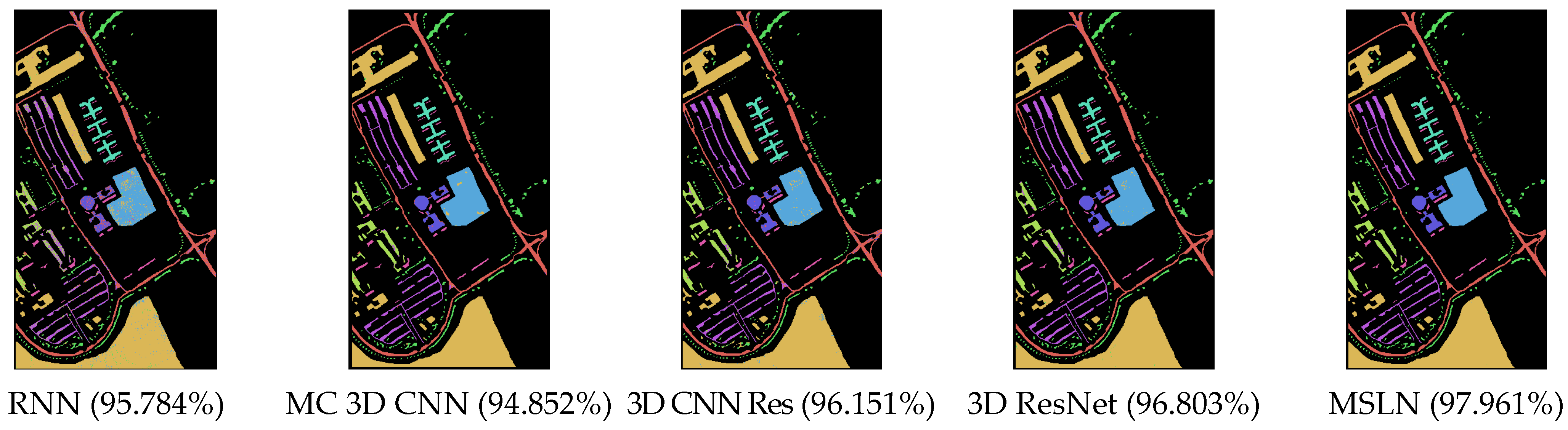
| Pavia University | 3D CNN | RNN | MC 3D CNN | 3D CNN Res | 3D ResNet | MSLN |
|---|---|---|---|---|---|---|
| 1 | 0.900 | 0.974 | 0.972 | 0.969 | 0.983 | 0.992 |
| 2 | 0.952 | 0.968 | 0.956 | 0.975 | 0.976 | 0.982 |
| 3 | 0.678 | 0.940 | 0.948 | 0.938 | 0.943 | 0.983 |
| 4 | 0.938 | 0.983 | 0.981 | 0.936 | 0.981 | 0.994 |
| 5 | 0.999 | 0.995 | 0.999 | 1.000 | 0.999 | 0.999 |
| 6 | 0.880 | 0.991 | 0.987 | 0.962 | 0.985 | 0.998 |
| 7 | 0.728 | 0.961 | 0.964 | 0.911 | 0.964 | 0.992 |
| 8 | 0.771 | 0.961 | 0.978 | 0.948 | 0.964 | 0.991 |
| 9 | 0.994 | 0.995 | 0.995 | 0.995 | 0.999 | 1.000 |
| Kappa | 0.865 | 0.945 | 0.933 | 0.949 | 0.958 | 0.973 |
| AA | 0.871 | 0.974 | 0.976 | 0.959 | 0.977 | 0.992 |
| OA (%) | 89.839 | 95.784 | 94.852 | 96.151 | 96.803 | 97.961 |
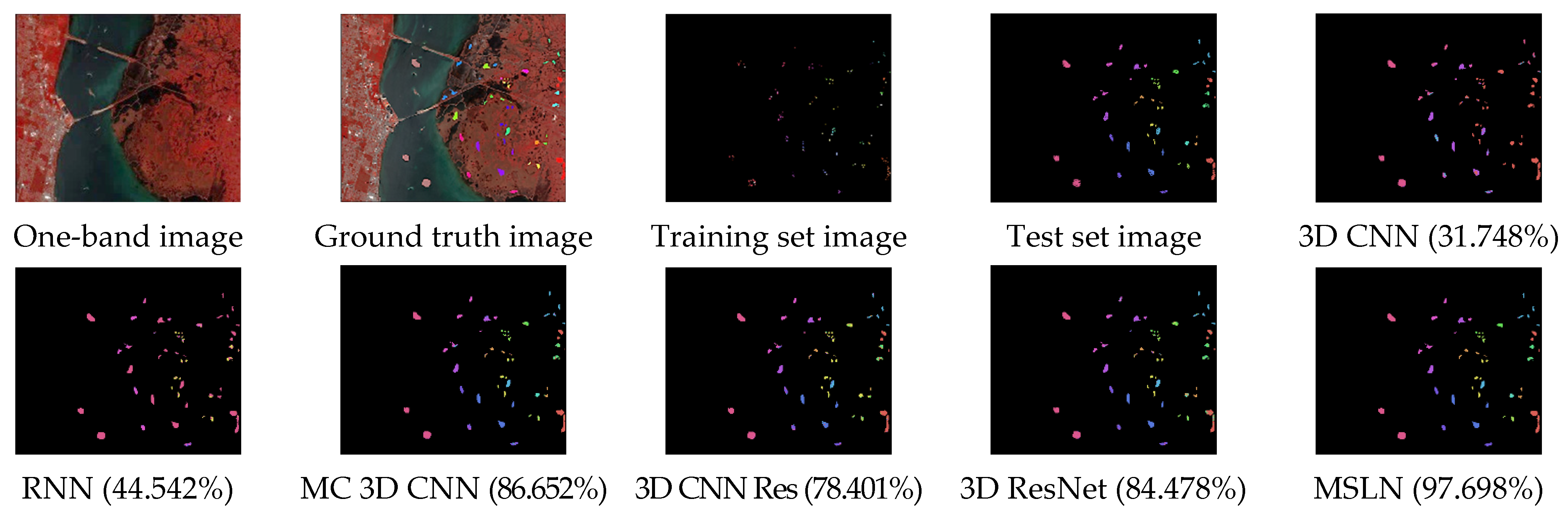
| KSC | 3D CNN | RNN | MC 3D CNN | 3D CNN Res | 3D ResNet | MSLN |
|---|---|---|---|---|---|---|
| 1 | 0.065 | 0.536 | 0.935 | 0.917 | 0.894 | 0.988 |
| 2 | 0.000 | 0.000 | 0.885 | 0.636 | 0.822 | 0.980 |
| 3 | 0.526 | 0.000 | 0.779 | 0.539 | 0.947 | 0.976 |
| 4 | 0.000 | 0.009 | 0.504 | 0.277 | 0.562 | 0.886 |
| 5 | 0.000 | 0.000 | 0.671 | 0.400 | 0.460 | 0.928 |
| 6 | 0.000 | 0.000 | 0.694 | 0.567 | 0.503 | 0.894 |
| 7 | 0.000 | 0.000 | 0.842 | 0.000 | 0.662 | 0.960 |
| 8 | 0.000 | 0.224 | 0.868 | 0.833 | 0.889 | 0.979 |
| 9 | 0.000 | 0.000 | 0.935 | 0.922 | 0.966 | 0.998 |
| 10 | 0.275 | 0.187 | 0.853 | 0.785 | 0.848 | 0.988 |
| 11 | 0.000 | 0.582 | 0.971 | 0.901 | 0.924 | 1.000 |
| 12 | 0.588 | 0.361 | 0.829 | 0.740 | 0.770 | 0.978 |
| 13 | 0.409 | 0.743 | 0.965 | 0.931 | 0.954 | 0.999 |
| Kappa | 0.200 | 0.360 | 0.852 | 0.759 | 0.827 | 0.974 |
| AA | 0.143 | 0.203 | 0.825 | 0.650 | 0.785 | 0.966 |
| OA (%) | 31.748 | 44.542 | 86.652 | 78.401 | 84.478 | 97.698 |
Publisher’s Note: MDPI stays neutral with regard to jurisdictional claims in published maps and institutional affiliations. |
© 2022 by the authors. Licensee MDPI, Basel, Switzerland. This article is an open access article distributed under the terms and conditions of the Creative Commons Attribution (CC BY) license (https://creativecommons.org/licenses/by/4.0/).
Share and Cite
Zheng, H.; Cao, Y.; Sun, M.; Guo, G.; Meng, J.; Guo, X.; Jiang, Y. Mixed Structure with 3D Multi-Shortcut-Link Networks for Hyperspectral Image Classification. Remote Sens. 2022, 14, 1230. https://doi.org/10.3390/rs14051230
Zheng H, Cao Y, Sun M, Guo G, Meng J, Guo X, Jiang Y. Mixed Structure with 3D Multi-Shortcut-Link Networks for Hyperspectral Image Classification. Remote Sensing. 2022; 14(5):1230. https://doi.org/10.3390/rs14051230
Chicago/Turabian StyleZheng, Hui, Yizhi Cao, Min Sun, Guihai Guo, Junzhen Meng, Xinwei Guo, and Yanchi Jiang. 2022. "Mixed Structure with 3D Multi-Shortcut-Link Networks for Hyperspectral Image Classification" Remote Sensing 14, no. 5: 1230. https://doi.org/10.3390/rs14051230
APA StyleZheng, H., Cao, Y., Sun, M., Guo, G., Meng, J., Guo, X., & Jiang, Y. (2022). Mixed Structure with 3D Multi-Shortcut-Link Networks for Hyperspectral Image Classification. Remote Sensing, 14(5), 1230. https://doi.org/10.3390/rs14051230