Article

Adaptive Square-Root Unscented Kalman Filter Phase Unwrapping with Modified Phase Gradient Estimation

1
Key Laboratory of Land Environment and Disaster Monitoring, MNR, China University of Mining and Technology, Xuzhou 221116, China
2
School of Environment Science and Spatial Informatics, China University of Mining and Technology, Xuzhou 221116, China
*
Author to whom correspondence should be addressed.
Remote Sens. 2022, 14(5), 1229; https://doi.org/10.3390/rs14051229
Submission received: 29 November 2021 / Revised: 5 February 2022 / Accepted: 28 February 2022 / Published: 2 March 2022
(This article belongs to the Special Issue Advances in InSAR Imaging and Data Processing)

Abstract

:
Phase unwrapping (PU) is a key program in data processing in the interferometric synthetic aperture radar (InSAR) technique, and its accuracy directly affects the quality of final SAR data products. However, PU in regions with large gradient changes and high noise has always been a difficult problem. To overcome the limitation, this article proposes an adaptive square-root unscented Kalman filter PU method. Specifically, a modified phase gradient estimation (PGE) algorithm is proposed, in which a Butterworth low-pass filter is embedded, and the PGE window can be adaptively adjusted according to phase root-mean-square errors of pixels. Furthermore, the outliers of the PGE results are detected and revised to obtain high-precision vertical and horizontal phase gradients. Finally, the unwrapped phase is calculated by the adaptive square-root unscented Kalman filter method. To the best of our knowledge, this article is the first to combine the modified PGE with an adaptive square-root unscented Kalman filter for PU. Two sets of simulated data and a set of TerraSAR-X/TanDEM-X real data were used for experimental verification. The experimental results demonstrated that the various improvement measures proposed in this article were effective. Additionally, compared with the minimum-cost flow algorithm (MCF), statistical-cost network-flow algorithm (SNAPHU) and unscented Kalman filter PU (UKFPU), the proposed method had better accuracy and model robustness.

1. Introduction

Interferometric synthetic aperture radar (InSAR) has been widely used in detecting crustal deformation [1,2,3], creating digital elevation models (DEMs) [4,5], etc. Phase unwrapping (PU) is an imperative step in data processing in the InSAR technique. To date, dozens of PU methods have been proposed [6]. However, the error in PU results is relatively great in regions with large gradient changes, and the robustness of PU methods is usually poor in high-noise regions, both of which are the research focus of the PU technique. Classical PU methods are limited by the phase continuity assumption [6], which makes it difficult to obtain ideal results in regions with large gradient changes. Although multi-baseline PU methods [7] can eliminate the limitations of the phase continuity assumption, there are still some difficulties in the baseline ratio and the acquisition of multi-baseline data. Therefore, it is important to develop a PU method that can obtain better PU results in regions with large gradient changes and high noise.
The minimum-cost flow algorithm (MCF) [8] and statistical-cost network-flow algorithm (SNAPHU) [9] are currently the most commonly used PU methods in engineering applications. These two methods can be classified into minimum-norm PU methods. Such algorithms are also represented by the least-squares method [10] and the LP-norm method [11], which essentially transform the PU into an optimization-based problem. Other classical PU methods are based on path-following, which are represented by branch-cut [12], region-growing [13] and minimum discontinuities [14]. Hence, some researchers have proposed many improvement measures based on the above methods [15,16,17] and even devised more innovative PU methods, such as PU methods based on the traveling salesman problem [18] and on the ant colony algorithm [19]. Lately, Yu et al. [20] proposed a novel minimum-infinity-norm-based PU method that could not only keep the fringe-congruency in the high-quality regions, but also filter the input phase fringes in the noisy regions. Tlili et al. [21] proposed a PU method based on energy minimization from contextual modeling, which considered both local and global constraints of the interferogram. Gao et al. [22] proposed a phase-slicing 2-D PU method using the -norm, which could effectively reduce the phase gradient interval. Accordingly, these novel methods have greatly broadened the research direction of PU.
The general PU methods need prefiltering, as incomplete filtering will cause the appearance of a large number of noise residuals, and excessive filtering will cause a loss of necessary phase information. Thus, PU methods based on Kalman filters have been extensively studied. The advantage of these methods is that filtering and unwrapping programs are run at the same time. Xie et al. [23,24] proposed an unscented Kalman filter (UKF) phase unwrapping (UKFPU) method and combined the maximum-likelihood phase gradient estimation (PGE) method and path-following strategy, which obtained ideal unwrapped results. In addition, Xie et al. [25] introduced the unscented information-filtering (UIF) model to the PU and combined the PGE method based on local frequency estimation and the heapsort algorithm, to further improve the efficiency of the unwrapping model and the accuracy of the unwrapped results. Similarly, Gao et al. [26] proposed an adaptive UKFPU method combined with median filtering that was more robust and could obtain relatively ideal unwrapped results in high-noise and low-coherence regions. Liu et al. [27] proposed a simplified cubature Kalman filter phase unwrapping (CKFPU) method. Compared to the UKFPU method, the CKFPU method does not need to set parameters when generating the sampling points. However, the operation of the programs may be easily blocked due to inappropriate selection of some parameters. For the particularity of the PU problem, the robustness and accuracy of the PU methods based on Kalman filtering still need to be further improved, especially in regions with large gradient changes and high noise.
One of the main factors for the vast majority of PU methods in obtaining high-precision results is whether accurate PGE results in the horizontal and vertical directions can be acquired. Particularly in regions with high noise and dense interferometric fringes, it is challenging to obtain extraordinarily effective PGE results. The multi-baseline PU methods, which eliminate the limitation of the phase continuity assumption due to expansion of the range of phase gradient ambiguity numbers, still rely on high-precision PGE results. In short, PGE has an extremely important impact on PU. The phase gradient information can be obtained by analyzing the interferometric fringe frequency of the interferogram. The classical fringe frequency estimation methods are mainly based on the phase difference [28,29], maximum likelihood (ML) [28,30], modified multiple-signal classification (MUSIC) [31,32], etc. The methods based on phase difference require the process of local PU. In regions with large gradient changes and high noise, the conventional PU methods cannot obtain the absolute phase of the local region correctly due to factors such as phase under-sampling, which causes inaccurate results of local fringe frequency estimation [28,33]. The ML and MUSIC-based methods assume that there is only one frequency in the estimation window, i.e., high-order frequencies are ignored. In addition, the size and shape of the estimation window will affect the accuracy of fringe frequency estimation [29]. Among the many PGE methods, ML-based local frequency estimation methods, such as the Amended Matrix Pencil Model (AMPM) [34], which consider both accuracy and efficiency, have been applied to many PU methods.
In view of the great errors in unwrapped results in regions with large gradient changes and high noise, this article proposes an adaptive square-root unscented Kalman filter phase unwrapping method, which is jointly abbreviated as the ASRUKFPU method. The ASRUKFPU method combines the modified PGE algorithm and the adaptive square-root unscented Kalman filter. To begin with, we have modified the PGE method based on local frequency estimation. On the one hand, we integrate the Butterworth low-pass filter into the PGE method; on the other hand, the PGE window can be adaptively selected on the basis of phase root-mean-square errors of interferogram pixels. Furthermore, in light of the frequency estimation results, we use a simple method to detect and revise the outliers. Finally, we employ an adaptive technique and square-root filtering to ameliorate the UKFPU method, i.e., the ASRUKFPU method. The processing results of the simulation data and real data show that the ASRUKFPU method has better unwrapped results and better model robustness in regions with large gradient changes and high noise than MCF, SNAPHU and UKFPU.
The rest of this article is organized as follows. In Section 2, the basic theories of PU and UKFPU are described. The modified PGE algorithm is presented in Section 3. Then, Section 4 provides a detailed implementation of the ASRUKFPU method. Section 5 analyzes the experimental results compared to those acquired with MCF, SNAPHU and UKFPU using simulated and TerraSAR-X/TanDEM-X real data, respectively. In Section 6, the advantages and limits of the proposed method are further discussed. Finally, conclusions are outlined in Section 7.

2. Phase Unwrapping Theory

2.1. Basic Theory of Phase Unwrapping

In general, the absolute phase is always wrapped in the interval ( π , π ] in a nonlinear way. The wrapping function [6] is shown below:
φ ( k ) = ψ ( k ) 2 n ( k ) π ,
where k represents the coordinate of the pixel, φ ( k ) and ψ ( k ) are the wrapped phase and absolute phase, respectively. n ( k ) represents the ambiguity number. To extract more reliable information from the phase of the signal, an appropriate integer multiple of 2 π must be allocated to the wrapped phase. For single-baseline PU methods, the phase gradient is limited by the phase continuity assumption:
Δ ψ ( k ) = [ φ ( k ) φ ( k 1 ) ] | 2 π ,
where Δ ψ ( k ) represents the PGE result of the absolute phase from pixel k to pixel k 1 obtained from the modulo 2π mapped wrapped phase-difference. Therefore, the change in phase gradient is limited to ( π , π ] When the phase is without noise, the PGE result of the absolute phase is equal to the PGE result of the wrapped phase. Consequently, the absolute phase of adjacent pixels can be calculated as:
ψ ( k ) = ψ ( k 1 ) + Δ ψ ( k ) = ψ ( k 1 ) + Δ φ ( k ) ,
where Δ φ ( k ) is the PGE result of the wrapped phase from pixel k to pixel k 1 . Ideally, the PGE results of the absolute phase can be obtained from the wrapped phase. Unfortunately, noise in the phase is so inevitable that PU cannot, in fact, be performed by estimating the phase gradients using Equation (2). Particularly in regions with large gradient changes and high noise, PGE becomes a difficult task. To address this issue, in this study, a modified PGE algorithm is proposed to obtain high-precision vertical and horizontal PGE results.

2.2. Unscented Kalman Filter Phase Unwrapping

Since the novel PU method proposed in this study is based on UKFPU, it is necessary to briefly introduce the UKFPU method here. The state and observation equations of the UKFPU mathematical model are shown in Equation (4). To facilitate the expression, we transform the two-dimensional UKFPU into a one-dimensional program to describe, and the one-dimensional coordinate k is used instead of the two-dimensional coordinate ( m ,   n ) of the pixel in the interferogram. Combined with the previous PU theory, from the relationship between the adjacent pixels in the interferogram and the characteristics of the interference complex signal, it can be obtained that:
{ ψ ( k ) = ψ ( k 1 ) + μ ( k 1 ) + ω ( k 1 ) = F [ ψ ( k 1 ) , k 1 ] + ω ( k 1 ) φ ( k ) = [ sin ( ψ ( k ) ) cos ( ψ ( k ) ) ] + [ υ 1 ( k ) υ 2 ( k ) ] = H [ ψ ( k ) ] + υ ( k ) ,
where μ ( k 1 ) is the real PGE result at pixel k 1 , ω ( k 1 ) is the estimation error of the phase gradient at pixel k 1 , and F [ ] represents the coefficient of the state equation. υ 1 ( k ) and υ 2 ( k ) are the variances of the observations, and H [ ] represents the coefficient of the observation equation.
Assume that ψ ¯ ( k 1 ) is the state estimation value at pixel k 1 , and P ¯ ( k 1 ) is the estimation error covariance of the state variable ψ ( k 1 ) . UKFPU approximates the distribution of the predicted values after the nonlinear transformation by selecting sigma points. For the state estimation value, the sigma points can be expressed as:
{ σ i = ψ ¯ ( k 1 )       i = 0 σ i = ψ ¯ ( k 1 ) + { ( N + η ) P ¯ ( k 1 ) } i i = 1 , ,   N σ i + N = ψ ¯ ( k 1 ) { ( N + η ) P ¯ ( k 1 ) } i i = 1 , ,   N ,
where { } i represents the i-th vector of the matrix in parentheses. N represents the dimension of the state variable (here N = 1 ), and η = τ 2 ( N + α ) N is the scale function, in which parameters τ and α are used to adjust the sigma points. τ determines the dispersion degree of the sigma points near the mean, and α is redundant. In this paper, we have set τ = 0.01 and α = 0 according to the previous reference [23]. Furthermore, the adjustment method can be found in [35]. The corresponding weight coefficients are:
{ w i p = η / ( N + η ) i = 0 w i q = η / ( N + η ) + ( 1 τ 2 + ζ ) i = 0 w i p = w i q = 1 / 2 ( N + η ) i = 1 , 2 , , 2 N ,
where w i p is the weight of the sigma point and the sigma point for predicted measurements, w i q is the weight used to calculate the prediction-value-error covariance matrix and predicted-measurements-error covariance matrix, and ζ is the parameter of nonlinear high-order information. For a Gaussian distribution, ζ = 2 is the best situation. Then, the sigma points will be passed through the function F [ ] , and the state estimation value of the predicted value and its estimation error covariance are calculated as:
{ χ i ( k ) = F [ σ i ( k 1 ) , k 1 ] i = 0 , 1 , , 2 N ψ ( k ) = i = 0 2 N w i p χ i ( k ) ,
P ψ ψ ( k ) = i = 0 2 N w i q [ χ i ( k ) ψ ( k ) ] [ χ i ( k ) ψ ( k ) ] T + Q ( k 1 ) ,
where χ i ( k ) represents the predicted value of the sigma point of pixel k in the interferogram, and ψ ( k ) is the state variable of pixel k . P ψ ψ ( k ) is the covariance of the state prediction error of pixel k , and Q ( k 1 ) represents the PGE error variance at pixel k 1 . Subsequently, the mean, covariance and cross-covariance of the sigma points are calculated by a nonlinear measurement function H [ ] :
{ φ i ( k ) = H [ χ i ( k ) ] φ ( k ) = i = 0 2 N w i p φ i ( k ) ,
P φ φ ( k ) = i = 0 2 N w i q [ φ i ( k ) φ ( k ) ] [ φ i ( k ) φ ( k ) ] T + R ( k ) ,
P ψ φ ( k ) = i = 0 2 N w i q [ χ i ( k ) ψ ( k ) ] [ φ i ( k ) φ ( k ) ] T ,
where φ i ( k ) represents the predicted observation, φ ( k ) is the measurement prediction value of pixel k , P φ φ ( k ) is the covariance of the measurement prediction, and P ψ φ ( k ) represents the covariance between the state variable and the measurement prediction. R ( k ) is the variance of the measurement error of pixel k . Eventually, it is necessary to calculate the Kalman gain matrix and update the state estimation value and its covariance:
g k = P ψ φ ( k ) / P φ φ ( k ) ,
ψ + ( k ) = ψ ( k ) + g k [ φ ( k ) φ ( k ) ] ,
P ψ ψ + ( k ) = P ψ ψ ( k ) g k P ψ φ ( k ) g k T ,
where g k represents the Kalman gain matrix of pixel k , ψ + ( k ) represents the state estimation value of pixel k , and P ψ ψ + ( k ) represents the covariance of the pixel-state estimation value of pixel k . The state estimation value ψ ¯ and error covariance P ¯ in Equation (5) are replaced by the state estimation ψ + in Equation (13) and error covariance P ψ ψ + in Equation (14), respectively; then, Equation (5) to Equation (14) are iteratively calculated until the state estimations of all the pixels of the interferogram are calculated.

3. Modified Phase Gradient Estimation Algorithm

Whether the PGE results of the interferogram can be accurately estimated is directly related to the accuracy of the PU results. The local frequency estimation method based on AMPM is a frequency estimation algorithm with good performance among the many PGE methods. AMPM assumes that the eigenvectors corresponding to the large eigenvalues are the useful phase signals, while the eigenvectors corresponding to the small eigenvalues are the non-signal components, i.e., noise. However, this assumption is not strict enough, because the boundary between large eigenvalues and small eigenvalues may not be clear. In addition, we find that there is an overcorrection phenomenon in AMPM, which leads to the loss of some useful phase information.
To explain the issue in more detail, we randomly deal with some pixels of certain simulated data by singular value decomposition (SVD) after implementing noise-free and noise-added conditions, respectively. Figure 1 shows the eigenvalue distribution of the signal matrix by SVD, in which the black curve represents the eigenvalue distribution in the presence of noise, and the blue curve is the eigenvalue distribution in the absence of noise. The AMPM algorithm directly subtracts the average of the remaining eigenvalues from the first eigenvalue of the black curve and then uses this value for a reconstruction calculation; it can be clearly seen that the value obtained is less than the first value of the blue curve, and the useful phase information represented by other eigenvalues on the blue curve is also discarded. This phenomenon normally exists when using the AMPM algorithm to estimate the phase gradient of pixels.

3.1. Modified PGE Based on Local Frequency Estimation

When the pixels are in an ideal state, i.e., the interferometric phase of the pixels does not contain noise, the large eigenvalues and small eigenvalues decrease markedly and the eigenvalues are considered to be well distributed. However, the interferometric phase of the actual pixels contains noise and the eigenvalues decrease evenly after SVD, which causes problems for eigenvalue processing. To suppress the influence of high-frequency noise on the PU while preserving the phase information as completely as possible, we propose the modified PGE algorithm based on local frequency estimation by using a low-pass filter (i.e., different weights are given to each eigenvalue) to solve the shortcomings of the AMPM algorithm.
There are many kinds of low-pass filters, and the effects of low-pass filters applied to local frequency estimation are different. The Butterworth filter, also known as the maximum flat filter, is characterized by a frequency response curve that is as flat as possible in the pass band without ripple, while it gradually decreases to zero in the stop band. Compared to other low-pass filters (e.g., Chebyshev low-pass filter), the Butterworth filter can assign more appropriate weights to large singularities and smaller weights to small singularities, which reduces high-frequency noise while retaining as much useful phase information as possible [36]. Therefore, a first-order Butterworth filter is used in this study to weight the singular values of the eigenvalue matrix. The specific implementation process is described as follows.
Based on the additive phase noise model, the complex interference signal Z t of pixel t can be expressed as:
Z t = exp [ j ( φ t + φ t n o i s e ) ] ,
where φ t represents the wrapped phase of pixel t , and φ t n o i s e is generally an independent random variable with the mean value of 0 and the standard deviation of ε υ . The interference complex signal is composed of multiple sine waves, and it is difficult to directly estimate all the frequency components. A local window can be used to calculate the main frequency, and assume that the frequency of the interference complex signal in the window is the same. Equation (15) can be expressed as:
Z t = exp [ j 2 π ( f t y r + f t x s ) ] = exp [ j ( Δ y r + Δ x s ) ] ,
where f t y and f t x represent the local frequency estimation results of the pixel in the azimuth and range in the window, with pixel t as the center. r and s represent the number of rows and lines of pixel t in the interferogram, respectively. Δ y and Δ x represent the phase gradient of azimuth and range in the local window, respectively.
Referring to Equation (16), when the frequency estimation results do not contain the noise frequency and the useful signal information is retained as much as possible, the estimation results of the phase gradient will be closer to the real PGE results. The modified PGE algorithm is as follows:
Assume that I t is the interferometric phase sample centered on pixel t , and the size of the window is L × L . First, the complex interference signal matrix I t is decomposed by SVD:
I t = U D V H ,
where U and V represent the L -order orthogonal unitary matrix, D is the corresponding eigenvalue matrix, and D = d i a g ( λ 1 ,   ,   λ L ) , λ 1 λ L 0 . The weight W h of the singular value is represented by the first-order Butterworth filter:
W h = 1 { 1 + [ ( a = 1 h λ a ) ( h λ h ) ] 2 } h = 1 ,   2 ,   ,   L .
The interferometric phase sample matrix I ¯ t is processed as:
I ¯ t = U ( W D ) V H ,
Then the parent Hankel matrix and two sub-Hankel matrices [24] are constructed according to the processed interferometric phase sample matrix I ¯ t , as follows:
{ I ˜ t 0 = I ¯ t ( 1 : L 1 ,   1 : L 1 ) I ˜ t 1 = I ¯ t ( 2 : L ,   1 : L 1 ) I ˜ t 2 = I ¯ t ( 1 : L 1 ,   2 : L ) ,
where, I ˜ t 0 , I ˜ t 1 and I ˜ t 2 are the parent Hankel matrix and two sub-Hankel matrices, respectively. The parent Hankel matrix I ˜ t 0 is decomposed by SVD again:
I ˜ t 0 = U ˜ 0 D ˜ 0 V ˜ 0 T ,
where U ˜ 0 , D ˜ 0 and V ˜ 0 only have information corresponding to the main eigenvalues related to the useful phase. The phase signal after dimensionality reduction can be obtained by SVD combined with Equation (20), as shown in Equation (22). Because the phase data matrix has a low rank structure, the noise can be suppressed after dimensionality reduction:
{ I t 0 = U ˜ 0 T I ˜ t 0 V ˜ 0 I t 1 = U ˜ 0 T I ˜ t 1 V ˜ 0 I t 2 = U ˜ 0 T I ˜ t 2 V ˜ 0 ,
where I t 0 , I t 1 and I t 2 are signal matrices reconstructed by the parent Hankel matrix and two sub-Hankel matrices. The local frequency estimation results of the range and azimuth of the sample in the window with pixel t as the center are as follows:
{ f t x = A r g ( c o n j ( I t 1 + I t 0 ) ) 2 π f t y = A r g ( c o n j ( I t 2 + I t 0 ) ) 2 π ,
where, I t 1 + and I t 2 + are pseudoinverse matrices [34] of I ˜ t 1 and I ˜ t 2 , respectively, and c o n j ( ) is the conjugate multiplication factor of the matrix.

3.2. Adaptive Window of PGE

The window selection of local frequency estimation is also the main content of PGE. The window of the frequency estimation is directly related to the results of the phase gradient, and then affects the accuracy of the PU results. The presupposition of the local frequency estimation method is that the interference fringes in the local regions are stationary. Therefore, in the process of local frequency estimation, the window of the frequency estimation must be considered to meet the presupposition. The slope of the terrain can reflect the fluctuation of the terrain. The interference fringes in the regions with large slopes are relatively dense, so we can set a small window to avoid destroying the assumption that the local fringes are stable, while the fringes in the regions with small slopes are relatively sparse, and a large window can be set up; this not only satisfies the assumption of local fringe stability, but also increases the number of sample pixels, which can improve the accuracy of the frequency estimation results. The root-mean-square error of the interferometric phase of the pixels can reflect the density of the fringes. If the fringes are dense, the root-mean-square error is large; otherwise, the root-mean-square error is small. Hence, the interferometric phase root-mean-square error can be used to adaptively select the window of the frequency estimation. The equation for calculating the root-mean-square error of the interferometric phase is:
ξ = sqrt [ a = 1 l × l ( A a A ¯ ) 2 / ( l × l ) ] ,
where l × l is a small window size to judge the density of fringes. A a represents the amplitude of the interferometric phase of the a-th pixel in the local window, A ¯ is the average of all A a in the local window, and ξ represents the interferometric phase root-mean-square error of the center pixel in the local window. In this study, we set up l = 5 . It is worth noting that for different interferograms, the ranges of the calculated root-mean-square error of the interferometric phase are different, but we can normalize them to approximately between 0 and 1 in a simple way. In this study, the size L × L of the local frequency estimation window is set as follows:
L × L = { 19 × 19 0 ξ < 0.5 17 × 17 0.5 ξ < 0.6 13 × 13 0.6 ξ < 0.8 9 × 9 0.8 ξ < 0.9 7 × 7 ξ 0.9 .

3.3. Detection and Revision of PGE Outliers

In regions with large gradient changes and high noise, the frequency estimation results are prone to errors. To improve the accuracy of the frequency estimation results, in this study, we propose a method to detect and revise the outliers of the frequency estimation results. In a small window, the frequency change of the local interference fringes is relatively small, and there will be no large jumps, so the frequency estimation results should be relatively continuous or even smooth. In fact, due to the factors such as large phase gradient changes, dense fringes and poor interferometric phase quality, there is an obvious discontinuity in the frequency estimation results in some local small regions. If the frequencies of these misestimated pixels are revised accurately, it can further help to improve the accuracy of the PU results. To begin with, it is necessary to identify the pixels whose frequency estimation results are abnormal. The continuity of the frequency estimates of the adjacent pixels in the range and azimuth can be determined by a sliding window, which aims to identify the pixels with abnormal frequency estimation results. We have specially developed an evaluation formula for this identification which discriminates outliers based on whether the local frequencies are consistent, as shown in Equation (26):
{ C f x = sqrt ( u = M M v = M M | f ( t + u , t + v ) x f t x | ) C f y = sqrt ( u = M M v = M M | f ( t + u , t + v ) y f t y | ) ,
where M is a parameter related to the window and is used for calculating continuity. In this study, we set up M = 3 , i.e., the size of the window is ( 2 M + 1 ) × ( 2 M + 1 ) = 7 × 7 . u and v represent the degree of deviation from the central pixel t . C f x and C f y represent the credible values of the frequency estimation results of pixel t in the range and azimuth, respectively. When the amount of noise in the interferogram is relatively small, the interference fringes in the local region are approximately stable, and the fringe frequency of the adjacent pixels remains unchanged; thus the values of C f x and C f y are small. In contrast, when the amount of noise in the interferogram is relatively large, the non-stationarity of the local interference fringes is enhanced, and the values of C f x and C f y are relatively large. When C f x and C f y are greater than the set threshold, the frequency estimation results of the pixel are unauthentic and need to be revised. It is not worth noting, but must be noted that the thresholds are set to C f x max / 2 and C f y max / 2 , where C f x max and C f y max represent the maximum values of C f x and C f y , respectively. When the credibility value exceeds the set threshold, the frequency estimation results of the pixel are replaced with the average frequency of all pixels in a window centered on pixel t as:
{ f ^ t x = 1 ( 2 M + 1 ) × ( 2 M + 1 ) u = M M v = M M f ( t + u , t + v ) x f ^ t y = 1 ( 2 M + 1 ) × ( 2 M + 1 ) u = M M v = M M f ( t + u , t + v ) y ,
where f ^ t x and f ^ t y represent the frequency estimation results of the revised pixels in the range and azimuth, respectively. Based on the revised local frequency estimation results, the high-precision PGE results of pixel t in range and azimuth can be obtained as:
Δ t x = 2 π f ^ t x   and   Δ t y = 2 π f ^ t y ,
where Δ t x and Δ t y are the final PGE results of the range and azimuth of pixel t , respectively.

4. Adaptive Square-Root Unscented Kalman filter PU Method

4.1. Square-Root Unscented Kalman Filter PU Method

Compared with the UKF algorithm, the square-root unscented Kalman filter (SRUKF) algorithm only needs the square root of the error covariance matrix for recursive calculation instead of a complete covariance matrix, which ensures the non-negative definiteness of the error covariance matrix, as reported in References [37,38]. Not only does it improve the numerical stability of the algorithm, but it also merely needs to calculate and save the square-root factor in the iterative calculation, which reduces the burden of computation. Hence, in this study, we introduce SRUKF to ameliorate the UKFPU technique. The square-root unscented Kalman filter PU (SRUKFPU) process is as follows:
Similar to the UKFPU method, assume that ψ ¯ ( k 1 ) is the state estimation value at pixel k 1 , and S ¯ ψ ψ ( k 1 ) is the square root of the error covariance of the state estimation value at pixel k 1 . For the state estimation value, the sigma points shown in Equation (5) will be changed to:
{ σ i = ψ ¯ ( k 1 ) i = 0 σ i = ψ ¯ ( k 1 ) + { N + η S ¯ ψ ψ ( k 1 ) } i i = 1 , , N σ i + N = ψ ¯ ( k 1 ) { N + η S ¯ ψ ψ ( k 1 ) } i i = 1 , , N
The corresponding weight coefficients are still calculated according to Equation (6). Then, the sigma points will be passed through the function F [ ] , and the state estimation value will still be calculated as Equation (7). However, the square root of state estimation error covariances will be calculated as:
{ S ψ ψ ( k ) = q r { w i q ( χ i ( k ) ψ ( k ) ) ,   Q ( k 1 ) } S ψ ψ ( k ) = c h o l u p d a t e { S ψ ψ ( k ) ,   χ 0 ( k ) ψ ( k ) ,   w 0 p } ,
where S ψ ψ ( k ) represents the square root of the covariance of the state prediction error of pixel k . q r { } and c h o l u p d a t e { } represent the QR decomposition operation and Cholesky divisor first-order update operation. Subsequently, the measurement prediction of pixel k is still calculated as Equation (9). The square root of the covariance of the measurement prediction is calculated as follows:
{ S φ φ ( k ) = q r { w i q ( φ i ( k ) φ ( k ) ) ,   R ( k ) } S φ φ ( k ) = c h o l u p d a t e { S φ φ ( k ) ,   φ 0 ( k ) φ ( k ) ,   w 0 p } ,
where S φ φ ( k ) represents the square root of the covariance of the measurement prediction at pixel k . The covariance between the state variable and the measurement prediction is also calculated as Equation (11). Finally, it is indispensable to calculate the Kalman gain matrix and update the state estimation value and the square root of its covariance.
g k = P ψ φ ( k ) / [ S φ φ ( k ) / S φ φ ( k ) ] ,
ψ + ( k ) = ψ ( k ) + g k [ φ ( k ) φ ( k ) ] ,
S ψ ψ + ( k ) = c h o l u p d a t e { S ψ ψ ,   g k S φ φ , 1 } ,
where S ψ ψ + ( k ) represents the square root of covariance of the state estimation value at pixel k . The state estimation value ψ ¯ and the square root of the error covariance of the state estimation value S ¯ ψ ψ in Equation (29) are replaced by the state estimation ψ + in Equation (33) and the square root of error covariance S ψ ψ + in Equation (34), respectively. Then, the above calculation program is repeated until the state estimations of all the pixels of the interferogram are calculated.

4.2. Adaptive Method

In the SRUKFPU method, the state and observation equations are relatively stationary, which might lead to the instability of the model because of high noise in practical applications. To address this issue and ensure the reliability of the observation information, in this section, we give the improvement measure of SRUKFPU. Needless to say, there are many adaptive techniques to refine Kalman filtering. For example, reference [39] lists four methods to determine the adaptive factors for balancing the contribution of kinematic model information and measurements. We hope that the measurement noise covariance can be adjusted adaptively, which is realized by judging the difference between the actual wrapped phase φ ( k ) and the predicted wrapped phase φ ( k ) . In other words, on the basis of SRUKFPU, we adopt the square root of the measurement-noise equivalent covariance matrix principle to make effective use of the observation information, following references [40,41].
Primarily, the predictive residual information is calculated as:
V ¯ k = φ ( k ) φ ( k ) ,
where V ¯ k is the predictive residual information of the pixel to be unwrapped. The diagonal elements of the equivalent covariance matrix for measurement noise covariance can be expressed in the form of IGIII:
R ¯ i ( k ) = { R i ( k ) | v i | U 0 R i ( k ) | v i | U 0 [ U 1 U 0 U 1 | v i | ] 2 U 0 < | v i | U 1 R i ( k ) 10 10 | v i | > U 1 ,
where R i ( k ) represents the i-th diagonal element of the measurement noise covariance matrix R ( k ) , and R ¯ i ( k ) represents the i-th diagonal element of the equivalent covariance matrix R ¯ ( k ) of the measurement noise covariance matrix. U 0 and U 1 are constant thresholds of decimal values, which can be set as needed. Routinely, 1.0 U 0 2.0 and 3.0 U 1 8.5 . v i is a standardized prediction residual, which can be acquired based on the variance divisor calculated by the median operation, as shown below:
{ v i = V ¯ k / ( σ k ( S φ φ S φ φ ) i ) σ k = 1.483 m e d i a n ( | V ¯ k | / ( S φ φ S φ φ ) i ) ,
where S φ φ is the square-root matrix of the covariance of the measurement prediction obtained by Equation (31). ( S φ φ S φ φ ) i represents the i -th diagonal element of the covariance matrix of the measurement prediction. m e d i a n ( ) is the median operator. The R ( k ) in Equation (31) will be replaced by the equivalent covariance matrix R ¯ ( k ) of the measurement noise covariance calculated by Equation (36), which will then participate in the iterative calculation of the SRUKFPU algorithms. As a result, outlier separation and revision of the square root of the measurement noise covariance may be realized; this has the ability to perfect the SRUKFPU, i.e., ASRUKFPU method. A schematic representation of the proposed ASRUKFPU method is shown in Figure 2. The main steps of the ASRUKFPU method are as follows:
Step 1. Phase gradient estimation: Use the modified PGE algorithm with the adaptive window to estimate the phase frequency of each pixel of the interferogram.
Step 2. Calculate the continuity of the phase frequency estimation results in Step 1, detect and revise the outliers, and use the revised results as the final PGE results.
Step 3. Phase unwrapping: The ASRUKFPU method is used to calculate the state estimation value of the waiting pixel and its square root of the corresponding covariance. If there are pixels waiting to be unwrapped, execute the ASRUKFPU method again; otherwise, end.

5. Experimental Results

5.1. Simulated Data Results

To evaluate the accuracy of the ASRUKFPU method, we used the simulated data as shown in Figure 3. The size of the simulated data was 256 × 256 pixels. We added 0.65 rad noise to the simulated wrapped phase, then the simulated noisy interferogram was processed by MCF, SNAPHU, UKFPU and ASRUKFPU. Since the added noise was random, we generated multiple noisy interferograms at the same noise level and unwrapped them by MCF. Then the interferograms with the best PU results of MCF were unwrapped by SNAPHU, UKFPU and ASRUKFPU methods. Figure 3a shows the three-dimensional display of the simulated topographic phase, Figure 3b is the corresponding unwrapped phase, Figure 3c is the simulated wrapped phase, and Figure 3d shows the simulated wrapped phase with noise that is to be unwrapped. The average coherence of the simulated interferogram after adding noise is 0.7180. To quantitatively evaluate the accuracy of the PU results, we calculated the mean absolute error (MAE) between the actual unwrapped phase and the simulated unwrapped phase:
MAE = 1 I × J m = 1 I n = 1 J | ψ ^ m , n ψ m , n | ,
where ψ ^ m , n represents the unwrapped phase at pixel (m, n), and ψm, n is the reference unwrapped phase. I and J are the number of rows and lines of the interferogram.
The unwrapped results of the four PU methods are shown in Figure 4, from which it can be seen that the PU results obtained by MCF and SNAPHU are not as smooth as those obtained by UKFPU and ASRUKFPU. In other words, the noise residuals of UKFPU and ASRUKFPU are significantly reduced after PU processing. From Figure 4c,f,i,l, we are able to see the estimation error distribution histograms of the unwrapped results of the four methods, in which we can see that the ASRUKFPU is significantly better than the other three PU methods; this is demonstrated by the fact that the error range of the ASRUKFPU is narrow, the errors are concentrated near 0 and have no large deviation, and the number of errors near 0 is maximum. Table 1 shows that the accuracies of MCF and SNAPHU are similar, but that their accuracies are obviously lower than those of UKFPU and ASRUKFPU, and the accuracy of ASRUKFPU is significantly higher than that of UKFPU. In CPU time consumption, the SNAPHU used in the experiment is in the Doris software, which is not in the same computer system as the other three methods; therefore, the unwrapping time of the SNAPHU is not counted. That the machine used was an Intel(R) with a speed of 3.6 GHz, 8GB RAM, on which the algorithms other than SNAPHU in this paper were conducted using MATLAB R2019b software. It can also be found from Table 1 that the unwrapping time of the UKFPU is the lowest and that of MCF is the longest. However, the unwrapping time of ASRUKFPU is slightly longer than that of UKFPU, which may be due to the addition of adaptive processing. Furthermore, the unwrapping time of ASRUKFPU is still in the same order of magnitude as that of the UKFPU method. From this experiment, it can be demonstrated that ASRUKFPU can obtain better unwrapped results, even in regions with large gradient changes and high noise.
In addition, based on the simulated dataset, we analyzed the improved parts of the ASRUKFPU. We combined the modified PGE with the adaptive window into the UKFPU but did not detect the continuity of the phase frequency estimation results, and revised the outliers. Using this method to unwrap the simulated noisy interferogram, the MAE of the unwrapped results is 0.1693 rad. In Table 1, the MAE of the unwrapped results of the UKFPU, combined with the local frequency estimation method based on AMPM, are 0.2674 rad; this indicates that the frequency estimation results of the modified PGE are more accurate than AMPM. Meanwhile, in Table 1, the MAE of the unwrapped results of ASRUKFPU, whose accuracy is higher than that of 0.1693 rad, are 0.1502 rad; this also indicates that the detection and revision of PGE outliers and adaptive square-root filtering are extraordinarily effective. Figure 5a,d are the PGE results of the simulated noise-free interferogram in the horizontal and vertical directions, respectively, which are also extremely close to the most ideal PGE results. Figure 5b,e are the PGE results of the simulated noisy interferogram in the horizontal and vertical directions, respectively, obtained by using the modified PGE algorithm; however, the frequency continuity detection and the revision of outliers were not carried out. The discontinuity of the phase gradient can be clearly seen from the red boxes. When the PGE results of Figure 5b,e were revised by the algorithm proposed in Section 3.3, they were more continuous and smoother, as shown in Figure 5c,f, whose results are also closer to the PGE results of Figure 5a,d than those of Figure 5b,e. These further prove that each improved part of the ASRUKFPU is effective.

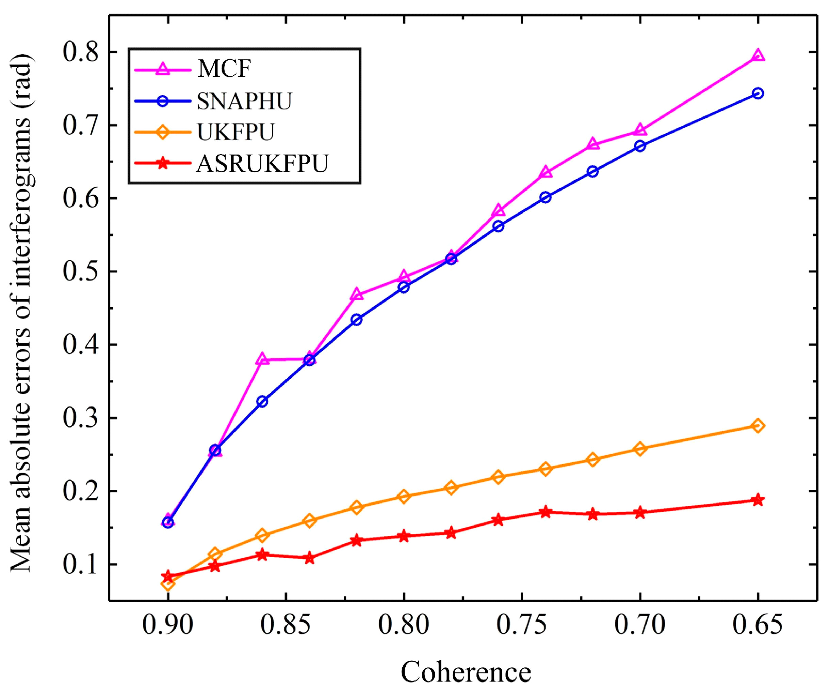
5.2. Robustness Analysis

The robustness analysis of PU models is also one of the main research tasks of the PU technique. To demonstrate the robustness of the ASRUKFPU method, we added different noises to another simulated dataset, as shown in Figure 6. It is worth noting that the noise was generated by the coherence of different mean values and obeyed hypergeometric distribution, which was closer to the actual noise than the white Gaussian noise [42]. Due to the addition of noise to the simulated interferogram, a small reduction in coherence occurred. Figure 6a is the three-dimensional display of the simulated terrain phase, and Figure 6b is the corresponding simulated unwrapped phase, in the middle of which we see an apparent topographic gradient change. Different amounts of noise were added to the simulated wrapped phase, and the phase coherence was set at 0.90, 0.88, 0.86, 0.84, 0.82, 0.80, 0.78, 0.76, 0.74, 0.72, 0.70, and 0.65, as shown in Figure 6c. Similarly, MCF, SNAPHU, UKFPU and ASRUKFPU were also used to process the series of noisy interferograms.
Accordingly, Figure 7 is a line chart for robustness analysis based on the unwrapped results of different PU methods. When the coherence of the simulated interferogram decreases, that is, the amount of noise increases, the unwrapping errors of the four PU methods all show a gradual increasing trend, while the increasing trends of MCF and SNAPHU are more prominent, and the increasing trends of UKFPU and ASRUKFPU are relatively gentle. Regarding the accuracy of the PU results, the MAE of ASRUKFPU is always the lowest with decreasing coherence. When the amount of noise is quite large, the MAE of ASRUKFPU is much lower than that of MCF and SNAPHU, and further, the MAE of ASRUKFPU is obviously lower than that of UKFPU. Consequently, this experiment demonstrates that ASRUKFPU is more robust than other pervasive methods and is more suitable for PU in regions with large gradient changes and high noise.

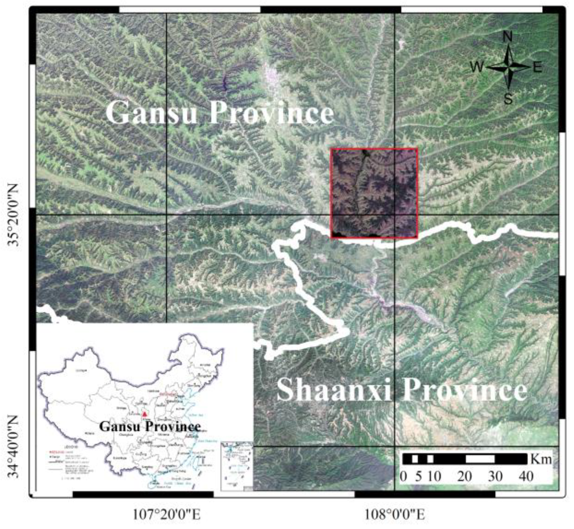
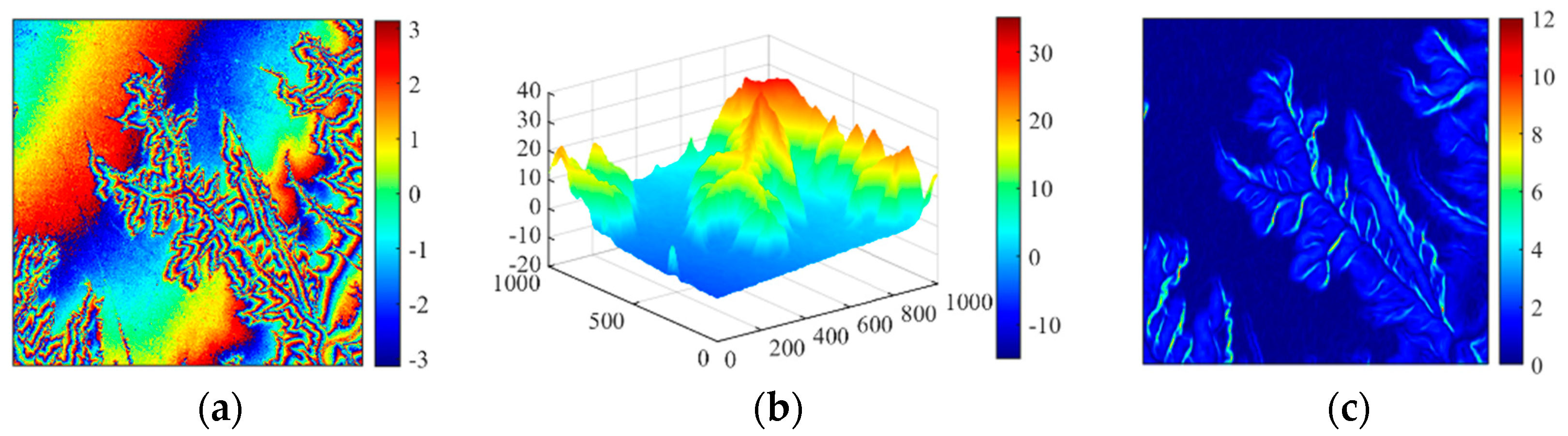
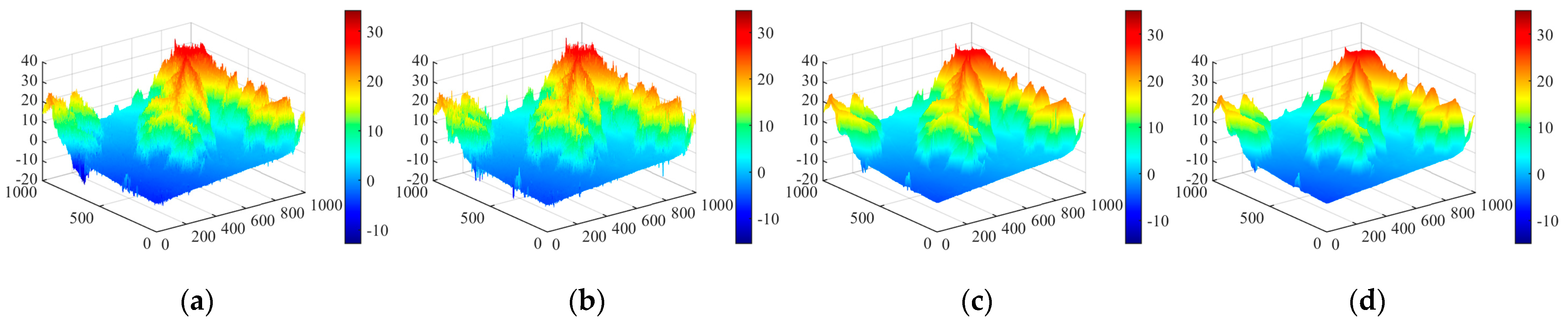
5.3. TerraSAR-X/TanDEM-X Data Results

To further demonstrate the effectiveness of the ASRUKFPU method, we selected the TerraSAR-X/TanDEM-X satellite images for experiments. The geographic location of the study area was at the junction of Qingyang City, Gansu Province, China; and Binzhou City, Shaanxi Province, China, as shown in Figure 8. The topography of the study area was the gully of the Loess Plateau. The difference between the minimum and maximum elevations of the study areas was about 300 m when the topography changed from loess flatlands to mountainous areas, which can reflect the topographic gradient changes to a certain extent.
The size of the experimental data in the satellite image was 4000 × 4000 pixels. Before PU processing, we performed 4 × 4 multi-looks on the real data and obtained the interferometric phase image after registration, removing the flat phase and other processing steps as shown in Figure 9a. The size of the interferogram after multi-looks was 1000 × 1000 pixels. From the interferogram, we can see that the interferometric fringes in the mountain areas are relatively dense and that there is a large number of noise residuals in these regions. On the one hand, the topographic slope change is relatively large and uneven in the mountain regions; on the other hand, the topographic slope changes sharply from the loess flatlands to the mountains, which provides advantageous conditions for us to certify the effectiveness of the ASRUKFPU method. Figure 9b is the reference unwrapped phase, generated by the Shuttle Radar Topography Mission (SRTM) DEM, which is used to evaluate the accuracy of diverse PU results. Assuming that the terrain inclination in a local small region is consistent, the phase estimation of the terrain slope can be calculated according to reference [29], as shown in Figure 9c.
Similarly, the interferogram was processed by MCF, SNAPHU, UKFPU and ASRUKFPU. Figure 10 is the 3D display of the results of different PU methods for TerraSAR-X/TanDEM-X data. The evaluation results of different methods on real data are shown in Table 2. It can be seen that all kinds of PU methods are affected by noise residual. However, the noise residuals after PU processing by UKFPU and ASRUKFPU are less than those by MCF and SNAPHU. Obviously, the noise residuals of ASRUKFPU are less than those of UKFPU, which shows that ASRUKFPU performs better in noise residual elimination. Thanks to the superior filtering performance of ASRUKF, it is the method with the fewest residuals among the four PU methods. Nevertheless, it is not sufficient to evaluate the effectiveness of the ASRUKFPU method only by comparing the number of noise residuals, because large gradient changes will also lead to noise residuals. To evaluate the accuracy of ASRUKFPU more effectively, we used Equation (38) to calculate the MAE between the unwrapped results of different PU methods and the reference unwrapped phase obtained from SRTM DEM.
Intuitively, Figure 10c differs slightly from Figure 10d. Therefore, we specifically created Figure 11 to analyze the error distribution of unwrapped results of different PU methods more directly, which was generated by adjusting the viewing angle of the 3D error map to (−45, 0). It is not worth noting but must be noted that the PU result is reliable when the error is concentrated around zero. From Figure 11, we can see that the error is mainly concentrated in the mountainous regions, and there are still many glitches in these areas after PU by MCF and SNAPHU. Although there are certain glitches in the PU results of UKFPU and ASRUKFPU, the error is significantly smaller than that of MCF and SNAPHU. It is also worth noting that the maximum and minimum unwrapping errors of MCF, SNAPHU and UKFPU are higher than those of the ASRUKFPU method, which seems to indicate that the revision of PGE outliers and the adaptive method are meaningful, ensuring that the unwrapping error will not deviate greatly. From Table 2, it can be seen that the PU accuracies of MCF and SNAPHU are similar, while the latter two PU methods obviously have higher accuracy, and the accuracy of ASRUKFPU is the highest among the four PU methods.
To demonstrate the advantages of the ASRUKFPU more intuitively, we extracted the PU results of a line of pixels in the interferogram as shown in Figure 12. Notably, the phase gradient of the line in the interferogram changes markedly, and the four PU methods can obtain the absolute phase as a whole. Furthermore, we intentionally marked two positions with black and red arrows in Figure 12, where we can clearly see the difference between the results of the PU methods. At the positions shown by the red arrows, it can be clearly seen that both MCF and SNAPHU have large PU errors, while UKFPU and ASRUKFPU can accurately calculate the absolute phase at the same position. In the positions shown by the black arrows, it is also obvious that MCF and SNAPHU have a large unwrapping error. Although UKFPU and ASRUKFPU also have a certain unwrapping error at this position, the unwrapped results of ASRUKFPU are closest to the ideal results by comparison. In addition, it can be seen from the values that the unwrapped results of ASRUKFPU at the positions indicated by the numerical values are closer to the ideal results than the unwrapped results of UKFPU. In conclusion, the unwrapped results of UKFPU and ASRUKFPU are better than those of MCF and SNAPHU. Hence, the unwrapped results of ASRUKFPU are better than those of UKFPU, to a large extent. The experiment further indicates that ASRUKFPU has a higher level of unwrapping accuracy and has better unwrapped results in regions with large gradient changes and high noise.

6. Discussion

The ASRUKFPU method proposed in this study is essentially a single-baseline PU method based on path-following. Therefore, the method will still not eliminate the limitation of the phase continuity assumption. However, there is no denying the fact that the various improvements proposed in this study are effective and meaningful. It is well known that one of the key steps in PU lies in the accurate estimation of the phase gradient. So long as the PGE results are sufficiently accurate, it seems possible to obtain satisfactory PU results according to the correct integral path. Hence, the modified PGE algorithm proposed in Section 3 aims to improve the accuracy of the PGE results, and the first set of simulation experiments also demonstrates that the algorithm and its various improved parts are effective. It is worth noting that the main purpose of introducing the Butterworth low-pass filter in this section is not for phase filtering, but to assist in the processing of singular values; this is to retain as many useful phase signals as possible, since the local phase frequency estimation algorithm based on SVD and the unscented Kalman filter method have been able to process the noisy interferograms. Additionally, the ASRUKFPU method enables the parallel processing of phase filtering and PU, so that the obtained unwrapped results are smoother and more accurate. Furthermore, another set of simulation experiments demonstrates that the model of the ASRUKFPU method is more robust. The test of TerraSAR-X/TanDEM-X real data shows that the accuracy of ASRUKFPU is improved by approximately 15% compared to UKFPU, and by about 30% compared to MCF, which is significative in practical engineering applications.
The ASRUKFPU method proposed in this study has great potential for the production of high-precision DEMs in local areas, especially for regions with elevation variations exceeding the ambiguous height (i.e., the elevation difference that can be represented by an interferometric phase period) and high noise. On the other hand, our method is also suitable for surface deformation monitoring, especially in regions with large deformation variables, e.g., mining areas, earthquake belts, volcanoes, etc. Lately, the deep-learning technique has been widely studied in PU, which broadens the research direction of PU. Next, we will try to combine deep learning with the ASRUKFPU method to obtain more satisfactory PU results, even in regions with large gradient changes and high noise.
Nevertheless, there still exists a problem in this article that needs to be further studied. In terms of computational efficiency, the computation of the ASRUKFPU method increases due to the addition of some improvement measures, which is also closely related to the implementation of the code to a certain degree. The authors are working on the problem and hope to resolve it in the near future.

7. Conclusions

In this research, the PU method based on an adaptive square-root unscented Kalman filter with a modified phase gradient estimation algorithm is proposed. Specifically, square-root filtering is introduced into UKFPU for the first time, and the Butterworth low-pass filter is applied to the PGE based on local frequency estimation in PU for the first time. In SRUKFPU, we also add an adaptive divisor to revise the outlier of the square root of the measurement noise covariance. Moreover, the window for calculating the phase gradient can be adaptively selected according to the phase root-mean-square error of the interferogram pixels, and the outliers of the PGE results can also be detected and revised. A set of simulated data experiments and a set of TerraSAR-X/TanDEM-X SAR image data experiments have demonstrated that ASRUKFPU has higher accuracy than MCF, SNAPHU and UKFPU. Another set of simulated data experiments indicates that ASRUKFPU has better model robustness and higher accuracy than the other three methods. Particularly in the regions with large topographic gradient changes and high noise, the unwrapped results of ASRUKFPU are better.

Author Contributions

Conceptualization, Y.Z. and Y.G.; methodology, Y.Z.; software, Y.Z.; validation, Y.Z., S.Z. and Y.G.; formal analysis, Y.G. and S.L.; investigation, Y.J.; resources, Y.G.; data curation, M.L.; writing—original draft preparation, Y.Z.; writing—review and editing, Y.Z. and Y.G.; visualization, S.L.; supervision, S.Z. and S.L.; project administration, S.Z. and Y.G.; funding acquisition, S.Z. and Y.G. All authors have contributed significantly and have participated sufficiently to take responsibility for this research. All authors have read and agreed to the published version of the manuscript.

Funding

This work was supported in part by the National Natural Science Foundation of China, grant number 42001409; in part by the China Postdoctoral Science Foundation 2020M681770; and in part by the Development Fund of the Key Laboratory of Land Satellite Remote Sensing Application Center, Ministry of Natural Resources of P.R. China, grant number KLSMNR-202103.

Institutional Review Board Statement

Not applicable.

Informed Consent Statement

Not applicable.

Data Availability Statement

The data are contained within the article.

Acknowledgments

The authors would like to thank the anonymous reviewers for their constructive comments and suggestions. The authors also thank the German Aerospace Center (DLR) for providing the TerraSAR-X/TanDEM-X data.

Conflicts of Interest

The authors declare that they have no conflict of interest.

References

  1. Chen, G.; Zhang, Y.; Zeng, R.; Yang, Z.; Chen, X.; Zhao, F.; Meng, X. Detection of land subsidence associated with land creation and rapid urbanization in the Chinese Loess Plateau using time series InSAR: A case study of Lanzhou new district. Remote Sens. 2018, 10, 270. [Google Scholar] [CrossRef] [Green Version]
  2. Caló, F.; Notti, D.; Galve, J.P.; Abdikan, S.; Görüm, T.; Pepe, A.; Balik Şanli, F. DInSAR-based detection of land subsidence and correlation with groundwater depletion in Konya Plain, Turkey. Remote Sens. 2017, 9, 83. [Google Scholar] [CrossRef] [Green Version]
  3. Jiang, J.; Lohman, R.B. Coherence-guided InSAR deformation analysis in the presence of ongoing land surface changes in the Imperial Valley, California. Remote Sens. Environ. 2020, 253, 112–160. [Google Scholar] [CrossRef]
  4. Rossi, C.; Gernhardt, S. Urban DEM generation, analysis and enhancements using TanDEM-X. ISPRS J. Photogramm. Remote Sens. 2013, 85, 120–131. [Google Scholar] [CrossRef]
  5. Dong, Y.; Jiang, H.; Zhang, L.; Liao, M. An efficient maximum likelihood estimation approach of multi-baseline SAR interferometry for refined topographic mapping in mountainous areas. Remote Sens. 2018, 10, 454. [Google Scholar] [CrossRef]
  6. Yu, H.; Lan, Y.; Yuan, Z.; Xu, J.; Lee, H. Phase unwrapping in InSAR: A review. IEEE Geosci. Remote Sens. Mag. 2019, 7, 40–58. [Google Scholar] [CrossRef]
  7. Yu, H.; Li, Z.; Bao, Z. A cluster-analysis-based efficient multibaseline phase-unwrapping algorithm. IEEE Trans. Geosci. Remote Sen. 2011, 49, 478–487. [Google Scholar] [CrossRef]
  8. Costantini, M. A novel phase unwrapping method based on network programming. IEEE Trans. Geosci. Remote Sens. 1998, 36, 813–821. [Google Scholar] [CrossRef]
  9. Chen, C.W.; Zebker, H.A. Two-dimensional phase unwrapping with use of statistical models for cost functions in nonlinear optimization. J. Opt. Soc. Am. A 2001, 18, 338–351. [Google Scholar] [CrossRef] [PubMed] [Green Version]
  10. Ghiglia, D.C.; Romero, L.A. Robust two-dimensional weighted and unweighted phase unwrapping that uses fast transforms and iterative methods. J. Opt. Soc. Am. A 1994, 11, 107–117. [Google Scholar] [CrossRef]
  11. Ghiglia, D.C.; Romero, L.A. Minimum Lp-norm two-dimensional phase unwrapping. J. Opt. Soc. Am. A 1996, 13, 1999–2013. [Google Scholar] [CrossRef]
  12. Zheng, D.; Da, F. A novel algorithm for branch cut phase unwrapping. Opt. Lasers Eng. 2011, 49, 609–617. [Google Scholar] [CrossRef]
  13. Xu, W.; Cumming, I. A region-growing algorithm for InSAR phase unwrapping. IEEE Trans. Geosci. Remote Sens. 1999, 37, 124–134. [Google Scholar] [CrossRef] [Green Version]
  14. Flynn, T.J. Two-dimensional phase unwrapping with minimum weighted discontinuity. J. Opt. Soc. Am. A 1997, 14, 2692–2701. [Google Scholar] [CrossRef]
  15. Zhong, H.; Tang, J.; Zhang, S.; Chen, M. An improved quality-guided phase-unwrapping algorithm based on priority queue. IEEE Geosci. Remote Sens. Lett. 2011, 8, 364–368. [Google Scholar] [CrossRef]
  16. Libert, L.; Derauw, D.; D’Oreye, N.; Barbier, C.; Orban, A. Split-Band Interferometry-Assisted Phase Unwrapping for the Phase Ambiguities Correction. Remote Sens. 2017, 9, 879. [Google Scholar] [CrossRef] [Green Version]
  17. Mao, W.; Wang, S.; Xu, B.; Li, Z.; Zhu, Y. An Improved Phase Unwrapping Method Based on Hierarchical Networking and Constrained Adjustment. Remote Sens. 2021, 13, 4193. [Google Scholar] [CrossRef]
  18. Karout, S.; Gdeisat, M.; Burton, D.; Lalor, M. Two-dimensional phase unwrapping using a hybrid genetic algorithm. Appl. Opt. 2007, 46, 730–743. [Google Scholar] [CrossRef]
  19. Wei, Z.Q.; Xu, F.; Jin, Y.Q. Phase unwrapping for SAR interferometry based on an ant colony optimization algorithm. Int. J. Remote Sens. 2007, 29, 711–725. [Google Scholar] [CrossRef]
  20. Yu, H.; Lan, Y.; Lee, H.; Cao, N. 2-D Phase Unwrapping Using Minimum Infinity-Norm. IEEE Geosci. Remote Sens. Lett. 2018, 15, 1887–1891. [Google Scholar] [CrossRef]
  21. Tlili, A.; Cavayas, F.; Foucher, S.; Siles, G.L. New interferometric phase unwrapping method based on energy minimization from contextual modeling. IEEE J. Sel. Top. Appl. Earth Observ. Remote Sens. 2020, 13, 6524–6532. [Google Scholar] [CrossRef]
  22. Gao, Y.; Tang, X.; Li, T.; Lu, J.; Li, S.; Chen, Q.; Zhang, X. A phase slicing 2-D phase unwrapping method using the L1-Norm. IEEE Geosci. Remote Sens. Lett. 2020, in press. [Google Scholar] [CrossRef]
  23. Xie, X.; Pi, Y. Phase noise filtering and phase unwrapping method based on unscented Kalman filter. J. Syst. Eng. Electron. 2011, 22, 365–372. [Google Scholar] [CrossRef]
  24. Xie, X.; Li, Y. Enhanced phase unwrapping algorithm based on unscented kalman filter, enhanced phase gradient estimator, and path-following strategy. Appl. Opt. 2014, 53, 4049–4060. [Google Scholar] [CrossRef]
  25. Xie, X.; Dai, G. Unscented information filtering phase unwrapping algorithm for interferometric fringe patterns. Appl. Opt. 2017, 56, 9423–9434. [Google Scholar] [CrossRef]
  26. Gao, Y.; Zhang, S.; Li, T.; Chen, Q.; Li, S.; Meng, P. Adaptive Unscented Kalman Filter Phase Unwrapping Method and Its Application on Gaofen-3 Interferometric SAR Data. Sensors 2018, 18, 1793. [Google Scholar] [CrossRef] [Green Version]
  27. Liu, W.; Bian, Z.; Liu, Z.; Zhang, Q. Evaluation of a Cubature Kalman Filtering-Based Phase Unwrapping Method for Differential Interferograms with High Noise in Coal Mining Areas. Sensors 2015, 15, 16336–16357. [Google Scholar] [CrossRef] [Green Version]
  28. Spagnolini, U. 2-D phase unwrapping and instantaneous frequency estimation. IEEE Trans. Geosci. Remote Sens. 1995, 33, 579–589. [Google Scholar] [CrossRef] [Green Version]
  29. Suo, Z.; Li, Z.; Bao, Z. A New Strategy to Estimate Local Fringe Frequencies for InSAR Phase Noise Reduction. IEEE Geosci. Remote Sens. Lett. 2010, 7, 771–775. [Google Scholar] [CrossRef]
  30. Wu, N.; Feng, D.; Li, J. A locally adaptive filter of interferometric phase images. IEEE Geosci. Remote Sens. Lett. 2006, 3, 73–77. [Google Scholar] [CrossRef]
  31. Trouve, E.; Caramma, M.; Maitre, H. Fringe detection in noisy complex interferograms. Appl. Opt. 1996, 35, 3799–3806. [Google Scholar] [CrossRef] [PubMed]
  32. Cai, B.; Liang, D.; Dong, Z. A new adaptive multiresolution noise-filtering approach for SAR interferometric phase images. IEEE Geosci. Remote Sens. Lett. 2008, 5, 266–270. [Google Scholar] [CrossRef]
  33. Ding, Z.; Wang, Z.; Lin, S.; Liu, T.; Zhang, Q.; Long, T. Local Fringe Frequency Estimation Based on Multifrequency InSAR for Phase-Noise Reduction in Highly Sloped Terrain. IEEE Geosci. Remote Sens. Lett. 2017, 14, 1527–1531. [Google Scholar] [CrossRef]
  34. Gao, Y.; Zhang, S.; Zhang, K.; Li, S. Frequency domain filtering SAR interferometric phase noise using the amended matrix pencil model. Comp. Model. Eng. Sci. 2019, 119, 349–363. [Google Scholar] [CrossRef] [Green Version]
  35. Lee, D. Nonlinear Estimation and Multiple Sensor Fusion Using Unscented Information Filtering. IEEE Signal Process. Lett. 2008, 15, 861–864. [Google Scholar] [CrossRef]
  36. Wang, G.; Wang, K. Study and design of exponential and Butterworth low-pass filters used for digital speckle interference fringe filtering. Optik 2013, 124, 6713–6717. [Google Scholar] [CrossRef]
  37. Holmes, S.A.; Klein, G.; Murray, D.W. An O(N²) Square Root Unscented Kalman Filter for Visual Simultaneous Localization and Mapping. IEEE Trans. Pattern Anal. Mach. Intell. 2009, 31, 1251–1263. [Google Scholar] [CrossRef]
  38. Menegaz, H.; Ishihara, J.Y.; Borges, G.; Vargas, A. A systematization of the unscented kalman filter theory. IEEE Trans. Autom. Control 2015, 60, 2583–2598. [Google Scholar] [CrossRef] [Green Version]
  39. Yang, Y.X.; Ren, X.; Xu, Y. Main progress of adaptively robust filter with applications in navigation. J. Navig. Position. 2013, 1, 9–15. [Google Scholar]
  40. Yang, Y.; Xu, T. An adaptive kalman filter based on sage windowing weights and variance components. J. Nav. 2003, 56, 231–240. [Google Scholar] [CrossRef]
  41. Wei, W.; Gao, S.; Zhong, Y.; Gu, C.; Hu, G. Adaptive square-root unscented particle filtering algorithm for dynamic navigation. Sensors 2018, 18, 2337. [Google Scholar] [CrossRef] [PubMed] [Green Version]
  42. Gao, Y.; Tang, X.; Li, T.; Chen, Q.; Zhang, X.; Li, S. Bayesian filtering multi-baseline phase unwrapping method based on a two-stage programming approach. Appl. Sci. 2020, 10, 3139. [Google Scholar] [CrossRef]
Figure 1. Singular values distribution.
Remotesensing 14 01229 g001
Figure 2. Schematic representation of the proposed adaptive square-root unscented Kalman filter phase unwrapping (ASRUKFPU) with modified phase gradient estimation method.
Remotesensing 14 01229 g002
Figure 3. Simulated data for PU accuracy verification (unit is rad): (a) three-dimensional display of the simulated terrain phase; (b) the simulated unwrapped phase; (c) the corresponding wrapped phase; (d) the interferogram calculated by adding noise into (c). The noise is 0.65 rad.
Remotesensing 14 01229 g003
Figure 4. Unwrapped maps (units are rad), PU error distribution maps (units are rad) and estimation error histograms: (ac) are the results obtained by MCF; (df) are the results obtained by SNAPHU; (gi) are the results obtained by UKFPU; (jl) are the results obtained by ASRUKFPU.
Remotesensing 14 01229 g004
Figure 5. PGE results (unit is rad). (a) PGE results of the simulated noise-free interferogram in the horizontal direction. (b) PGE results of the simulated noisy interferogram in the horizontal direction by using the modified PGE method, but the continuity detection and the revision of outliers are not carried out. (c) PGE results after revision for outliers in the horizontal direction. (d) PGE results of the simulated noise-free interferogram in the vertical direction. (e) PGE results in the vertical direction corresponding to (b). (f) PGE results after revision for outliers in the vertical direction.
Remotesensing 14 01229 g005
Figure 6. More simulated data for robustness analysis (unit is rad): (a) three-dimensional display of simulated terrain phase; (b) the simulated unwrapped phase; (c) noisy interferograms obtained by adding noise according to coherence values from 0.90 to 0.65.
Remotesensing 14 01229 g006
Figure 7. The robustness analysis line graph of different PU methods.
Remotesensing 14 01229 g007
Figure 8. Geographic location of the study area.
Remotesensing 14 01229 g008
Figure 9. Experimental dataset (unit is rad): (a) TerraSAR-X/TanDEM-X interferogram; (b) reference PU result of (a) obtained from SRTM DEM; (c) phase estimation of terrain slope.
Remotesensing 14 01229 g009
Figure 10. Experimental results for TerraSAR-X/TanDEM-X data (unit is rad): (a) PU result obtained by MCF; (b) PU result obtained by SNAPHU; (c) PU result obtained by UKFPU; (d) PU result obtained by ASRUKFPU.
Remotesensing 14 01229 g010
Figure 11. The unwrapping error display of different methods by adjusting the viewing angle of the 3D error map to (−45, 0): (a) difference between Figure 9b and Figure 10a; (b) difference between Figure 9b and Figure 10b; (c) difference between Figure 9b and Figure 10c; (d) difference between Figure 9b and Figure 10d. Note: unit of the color bar is rad.
Remotesensing 14 01229 g011
Figure 12. The PU results of a line of the pixels in the actual interferogram.
Remotesensing 14 01229 g012
Table 1. The evaluation results of different methods on simulated data.
MethodsTime (s)Error Range (rad)MAE (rad)
MCF8.37[−6.1326, 7.2449]0.5995
SNAPHU-[−4.0745, 4.3385]0.5941
UKFPU1.07[−1.7752, 1.9319]0.2674
ASRUKFPU3.03[−2.0349, 1.3972]0.1502
Table 2. The evaluation results of different methods on TerraSAR-X/TanDEM-X data.
MethodsResidualsError range (rad)MAE (rad)
MCF20,255[−15.7956, 14.6263]0.8411
SNAPHU20,255[−20.3866, 15.5055]0.7822
UKFPU2624[−14.4530, 16.3758]0.6981
ASRUKFPU2253[−11.5615, 11.7899]0.5948
Publisher’s Note: MDPI stays neutral with regard to jurisdictional claims in published maps and institutional affiliations.

