Functional Analysis for Habitat Mapping in a Special Area of Conservation Using Sentinel-2 Time-Series Data

Abstract

The mapping and monitoring of natural and semi-natural habitats are crucial activities and are regulated by European policies and regulations, such as the 92/43/EEC. In the Mediterranean area, which is characterized by high vegetational and environmental diversity, the mapping and monitoring of habitats are particularly difficult and often exclusively based on in situ observations. In this scenario, it is necessary to automate the generation of updated maps to support the decisions of policy makers. At present, the availability of high spatiotemporal resolution data provides new possibilities for improving the mapping and monitoring of habitats. In this work, we present a methodology that, starting from remotely sensed time-series data, generates habitat maps using supervised classification supported by Functional Data Analysis. We constructed the methodology using Sentinel-2 data in the Mediterranean Special Area of Conservation “Gola di Frasassi” (Code: IT5320003). In particular, the training set uses 308 field plots with 11 target classes (five forests, two shrubs, one grassland, one mosaic, one extensive crop, and one urban land). Starting from vegetation index time-series data, Functional Principal Component Analysis was applied to derive FPCA scores and components. In particular, in the classification stage, the FPCA scores are considered as features. The obtained results out-performed a previous map derived from photo-interpretation by domain experts. We obtained an overall accuracy of 85.58% using vegetation index time-series, topography, and lithology data. The main advantages of the proposed approach are the capability to efficiently compress high dimensional data (dense remote-sensing time series) providing results in a compact way (e.g., FPCA scores and mean seasonal time profiles) that: (i) facilitate the link between remote sensing with habitat mapping and monitoring and their ecological interpretation and (ii) could be complementary to species-based approaches in plant community ecology and phytosociology.

1. Introduction

Phytosociology (i.e., the Floristic–Sociologic Approach to Vegetation Classification [1]) is the most widespread method of studying and classifying vegetation in Europe [2,3]. Plant communities, called plant associations, are the most detailed discrete units recognized in phytosociology. These plant associations, recurring in space and time, are characterized by a distinct floristic composition that reflects the current and past ecological–environmental conditions (e.g., bioclimatic features, biogeography, topographic conditions, lithology, and land-uses) [4].

Plant associations and the higher levels of phytosociological vegetation classification (classes, orders, and alliances) are useful for the diagnosis of most natural and semi-natural habitats listed in Annex I of the Habitats Directive [5,6]. Plant association mapping allows for understanding of the spatial distribution of the habitats and, if repeated over time, to evaluate and monitor their conservation status.

Therefore, these activities are useful for achieving the goals set out in European environmental policies (e.g., Directive 92/43/CEE) [7,8,9,10]. Due to the high heterogeneity, fragmentation, and diversity of vegetation, the mapping and monitoring of Mediterranean plant associations and habitats are particularly challenging, when relying only on in situ observations [10,11,12].

This challenge can be supported by remote-sensing data, which, combined with field plots, enables the accurate mapping of plant communities and habitats [13,14,15,16]. The processing of remotely sensed data provides a better understanding of the conservation status, which is crucial in helping decision makers to plan and evaluate the impacts of management practices [9,17,18,19,20].

Mapping based on remote data is effective and accurate, if multi-temporal data are used to capture the seasonal variations of the spectral reflectance, in relation to the different phenological stages of the vegetation (i.e., vegetation seasonality) [11,14,16,21,22,23,24]. In contrast, mapping based on the spectral information of a single scene (i.e., single-date mapping) can be problematic, as distinct types of vegetation and habitats could have high spectral similarities at a given time of the season [25,26], even in multi-spectral data scenarios.

The growing availability of remote-sensing open data (e.g., Landsat, Sentinel, and MODIS) in formats usable by non-specialists (see, e.g., [27]) has facilitated the use of multiple images and dense time-series for various purposes. Dense time-series can capture the variations (both seasonal and inter-annual) of reflectance spectral bands or vegetation indices (e.g., NDVI) and are useful for the characterization of land-cover, ecosystem phenology, and landscape dynamics [28].

The use of dense time-series (>30 images per year) significantly improves the discrimination and mapping of natural vegetation types compared to using multi-temporal imagery (consisting of only a few images per year) [26,29]. Lopes et al. [26] considered the analysis of dense time-series as the new norm for tracking changes in the distribution of natural vegetation from space. Furthermore, considering entire archives of remotely sensed images (e.g., Landsat and Sentinel-2) as a cohesive temporal record, rather than as a series of individual images, provides new ecologically relevant perspectives [30].

The analysis of remotely sensed time-series plays a key role, and Functional Data Analysis (FDA) represents a reliable opportunity to analyze temporal ecological data, such as remotely sensed time-series [31]. FDA methods consider a time-series or a series (stack) of a remotely sensed images as a unique and cohesive temporal record. The basic philosophy of FDA is to consider observed data functions as single entities, rather than merely as a sequence of individual observations. The pixels to be processed are treated as temporal curves and, hence, as functions.

One of the most popular FDA methods is Functional Principal Component Analysis (FPCA) [32]. FPCA is a reduction tool that adapts traditional PCA concepts to functions. FPCA, unlike PCA, preserves the order in the data (e.g., the chronological order in the time-series) [33]. FDA techniques have been gaining in popularity in several scientific fields, ranging from genomics to finance [34]. This tool is still rarely used in remote sensing and ecology, despite some promising applications.

Li et al. [35] adopted the FPCA to classify Hyperspectral Images, considering that FDA treats multivariate data as continuous functions. Hurley et al. [31] applied FPCA to NDVI time-series to test the effects of spring and autumn phenology on the winter survival of mule deer fawns. The analysis of dense remotely sensing time-series with the functional approach has recently opened new avenues for plant association and habitat mapping as well as for the integration of remote sensing and phytosociology.

Pesaresi et al. [36] used the main seasonal NDVI variations, extracted from NDVI Landsat 8 dense time-series by FPCA, to recognize and characterize forest plant associations identified on the ground by the phytosociological approach; while, in Pesaresi et al. [37], the main seasonal NDVI variations were used (as input data and spatial predictors) together with a Random Forest classifier to map four forest plant associations in a coastal Mediterranean area of central Italy, obtaining a global accuracy of approximately 87%.

In this work, we evaluate the performance and applicability of the methodology proposed by Pesaresi et al. [37] in order to map the plant associations and habitats of a Special Area of Conservation (SAC ‘IT5320003’—Gola di Frasassi), located in a mountainous sector of central Italy and characterized by high vegetation, topographic, and lithological diversity.

To achieve this goal, we applied: (i) FPCA to Sentinel-2 dense time-series of different spectral-band-based vegetation indices (e.g., NDVI, NDWI) in order to identify the main seasonal spectral reflectance variations (FPCA components); (ii) (classical) PCA to a set of topographic terrain parameters (extracted from a Digital Elevation Model) and to lithological types in order to identify the main topographic and lithological features (PCA components); and, finally, (iii) supervised classification (by Random Forest) of the FPCA and PCA components in order to map the plant associations and habitats.

2. Materials and Methods

In this section, we provide details regarding the materials and methods of our approach. Figure 1 shows the adopted pipeline, which processes Sentinel-2 time-series data to derive maps of plant associations and habitats.

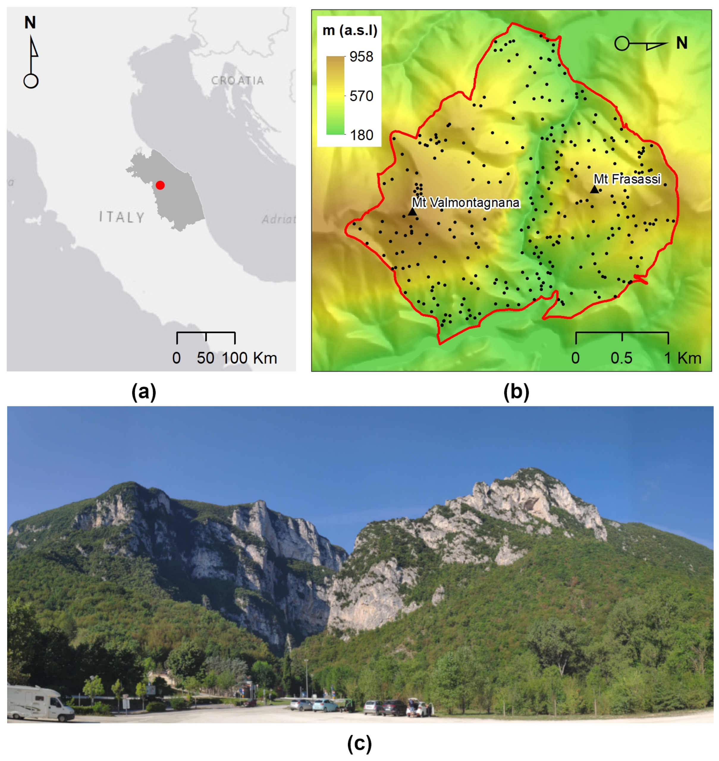
2.1. Study Site

The study area is the Special Area of Conservation (SAC) Gola di Frasassi (also known as the Gorge of Frasassi; code IT5320003). It is located in the mountainous area of the central Apennines (between latitudes of ${43}^{\circ }{23}^{\prime }{06}^{″}$ N–${43}^{\circ }{24}^{\prime }{50}^{″}$ N and longitudes of ${12}^{\circ }{55}^{\prime }{50}^{″}$ E–${12}^{\circ }{58}^{\prime }{46}^{″}$ E), along the Sentino River between Mount Valmontagnana (935 m a.s.l.) and Mount Frasassi (709 m a.s.l.).

The area is characterized by a high topographical and lithological heterogeneity. It encompasses an area of about 728 hectares (Figure 2). The average annual precipitation is 1115 mm, while the average annual temperature is 12.7 °C. According to the bioclimatic classification of Rivas-Martinez et al. [38], the area belongs to the temperate macrobioclimate with a weak sub-Mediterranean level, which indicates low summer aridity [39].

2.2. Target Classes and Reference Data

The following section describes the plant associations, recognized through the floristic-sociological approach of Braun–Blanquet and the corresponding habitats of Directive 92/43/EEC.

Woodland: (i) Holm-oak woods (habitat 9340 “Quercus ilex and Quercus rotundifolia forests”). Appenninic holm-oak woods differ from coastal or sub-coastal ones as they are richer in deciduous species (e.g., Fraxinus ornus L., Acer opalus subsp. obtusatum (Waldst. and Kit. ex Willd.) Gams, Sorbus domestica L., S. torminalis (L.) Crantz, Ostrya carpinifolia Scop.) in the tree layer and, in the understory, mesophilous species occur, such as Melica uniflora Retz., Hepatica nobilis Mill., and some orchids, among others. These species are typical of the deciduous woods surrounding holm-oak woods and easily enter in these as well.

At the same time, the most thermophilic species are lost or become rare (e.g., Rosa sempervirens L., Rhamnus alaternus L., and Pistacia lentiscus L.), as they cannot bear the rigors of the winter season. Therefore, they are classified in the association named Cephalanthero longifoliae-Quercetum ilicis, which represents the most mesophilous community of holm-oak woods, at least in the central Apennines [40]. They are widespread throughout the area, above and all along the vertical walls of the rocky gorge.

(ii) Downy-oak (Quercus pubescens Wiild.) woods (habitat 91AA* “Eastern white oak woods”). In the inland areas, downy oak woods occur on poor, eroded, and stony soils, forming open, sometimes degraded, woods with a thick herb layer and including several shrub species (i.e., Cytisophyllum sessilifolium (L.) O. Lang, Juniperus oxycedrus L., Cotinus coggygria Scop., and Pistacia terebinthus L.). These woods belong to the association Cytiso sessilifolii-Quercetum pubescentis, representing the typical downy oak woods of sub-montane areas on limestones  [41,42].

(iii) Black hornbeam forests occurring in the study area are classified within the association Scutellario columnae-Ostryetum carpinifoliae, which has a very large ecological amplitude, as it occurs in different ecological conditions. Indeed, on rocky slopes, it hosts species of the Mediterranean biocora, such as Q. ilex while, in mesic environments, it is richer in nemoral species of the Temperate biocora (e.g., Fagus sylvatica L. and S. torminalis). Black hornbeam forests are not recognized as habitats by the European Directive.

(iv) Riparian woods occur along the Sentino river flowing in the lower part of the rocky gorge. These are linear wood formations of white willow (Salix alba L.; of the association Rubo ulmifolii-Salicetum albae) growing along the river banks and of black poplar (Populus nigra L.) in the alluvial terrace above (Salici-Populetum nigrae). Both communities belong to the habitat 92A0 “Salix alba and Populus alba galleries”.

(v) Pinus sp. pl. plantation. In the Apennines, huge plantations of Pinus sp. pl. and other conifers have been found in the past few centuries. In the study area, Pinus nigra ssp. nigra Arnold and P. halepensis Mill. plantations are common throughout the whole area, especially on eroded soil along the steepest slopes [43].

Shrublands: These are widespread throughout the study area, occurring on abandoned grasslands as dynamic stages of wood recolonization. In areas with deeper soils, the main common species is Spartium junceum L. and, secondarily, C. sessilifolium. Together, they form the association Spartio juncei-Cytisetum sessilifolii, which is widespread in the central Apennines. On thinner and poorer soils, the dominant species is Juniperus oxycedrus, constituting wide shrublands in the area. They are framed in the same association as the previous one but with the J. oxycedrus variant [44].

Grasslands: While grasslands are not particularly widespread in the area, the most consistent nucleus is located at the top of Mount Valmontagnana, where cattle breeding is still practiced. However, these are rather sparse and arid meadows, due to the strong stonyness of the substrate and the low depth of the soil. The reference association is Asperulo purpureae-Brometum erecti, which belongs to priority habitat 6210(*) “Semi-natural dry grasslands and scrubland facies on calcareous substrates (Festuco-Brometalia) (*important orchid sites)” [45].

Garrigues and vegetation of rock and scree: These are strictly interpenetrated and, therefore, have been mapped as a mosaic. Garrigues are formed by dwarf chamaephytes, such as Satureja montana L., Fumana thymifolia (L.) Spach ex Webb, and Thymus sp. pl., occurring on eroded soil and rocky outcrops where they form the association Cephalario leucanthae-Saturejetum montanae [45,46]. Habitats 6110 “Rupicolous calcareous or basophilic grasslands of the Alysso-Sedion albi” and 6220 “Pseudo-steppe with grasses and annuals of the Thero-Brachypodietea” are present in the clearings of this vegetation.

On shady and wet rocky walls, particularly along the gorge’s wall, chasmophytic vegetation occurs (habitat 8210 “Calcareous rocky slopes with chasmophytic vegetation”), belonging to the association Moehringio papulosae-Potentilletum caulescentis. Other mapped typologies are crop lands, mainly represented by cereal crops, and urban land comprised of small towns, villages, and scattered houses.

The collected reference data, distributed over the study area (Figure 2), was based on 308 plots and used as training data for supervised plant association mapping (see

Table 1. Reference data. Target classes for the supervised map are listed. For plant associations, we report the syntaxa name and the corresponding habitat code (Annex 1 of the European Union Habitats Directive). The * denotes a priority habitat. In the case of 6210 if is an important orchid sites (*).

Class	Plant Association (Syntaxa)	Habitat Code	Plots
	Woodland
1	Holm-oak wood (Cephalanthero longifoliae-Quercetum ilicis)	9340	37
2	Downy-oak wood (Cytiso sessilifolii-Quercetum pubescentis)	91AA *	34
3	Black hornbeam wood (Scutellario columnae-Ostryetum carpinifoliae)	-	60
4	Pinus sp. plantations	-	32
5	Riparian woods (Rubo ulmifolii-Salicetum albae and Salici-Popolutem nigrae)	92A0	16
	Shrublands
6	Spartium junceum shrub (Spartio juncei-Cytisetum sessilifolii Spartium junceum variant)	-	16
7	Juniperus oxycedrus shrub (Spartio juncei-Cytisetum sessilifolii Juniperus oxycedrus variant)	-	15
	Grasslands
8	Bromus erectus grassland (Asperulo purpurei-Brometum erecti)	6210 (*)	16
	Mosaic of garrigues and chasmophytic vegetation
9	Garrigues and vegetation of rock and scree (Cephalario leucanthae-Saturejetum montanae and Moehringio papulosae-Potentilletum caulescentis)	6110, 6220, 8210	49
	Other
10	Crop land	-	18
11	Urban land	-	15

). Phyto-sociological surveys were performed in 74 plots (during 2018 and 2019) in order to identify the different plant associations and their mean specific composition. Subsequently, another 94 plots, through an expert-based similarity comparison in the field, were assigned to the identified plant associations. Finally, 140 plots were assigned to the target classes by visual interpretation of Google Earth imagery. The data set and R code used in the study are available from [47].

2.3. Topographic and Lithological Factors

Two different groups of ancillary features were included in the classifications: topography and lithology. Topography and lithology are natural factors that influence the composition of plant communities, as well as their spatial distribution [48].

Table 2. Lithology and terrain parameters used as predictors in this work, derived from a Digital Elevation Model using the System for Automated Geoscientific Analyses (SAGA) GIS software.

Type	Description
Terrain Parameters	Altitude (m a.s.l) Slope of the terrain (°) Topographic Position Index (TPI) Topographic Wetness Index (TWI) Northness Eastness Incoming solar radiation
Lithology	“Calcare Massiccio” formation; micritic limestone:“Bugarone” and “Maiolica formation”; marly-calcareous formation; landslide deposits; slope deposits; alluvial deposits

summarizes the terrain topographic parameters (quantitative data), extracted from a DEM with 30 m resolution (the DEM was derived from the NASA Shuttle Radar Topography Mission (SRTM)) and the lithological types (qualitative data derived from the lithological map of the Marche Region [49]).

Lithology and terrain parameters were processed by the Principal Component Analysis for mixed data (quantitative and qualitative) (dudihillsmith() of ade4 [50]). The obtained PCA scores were used as input (predictors) for modeling plant associations and habitats using a supervised Random Forest (RF) algorithm.

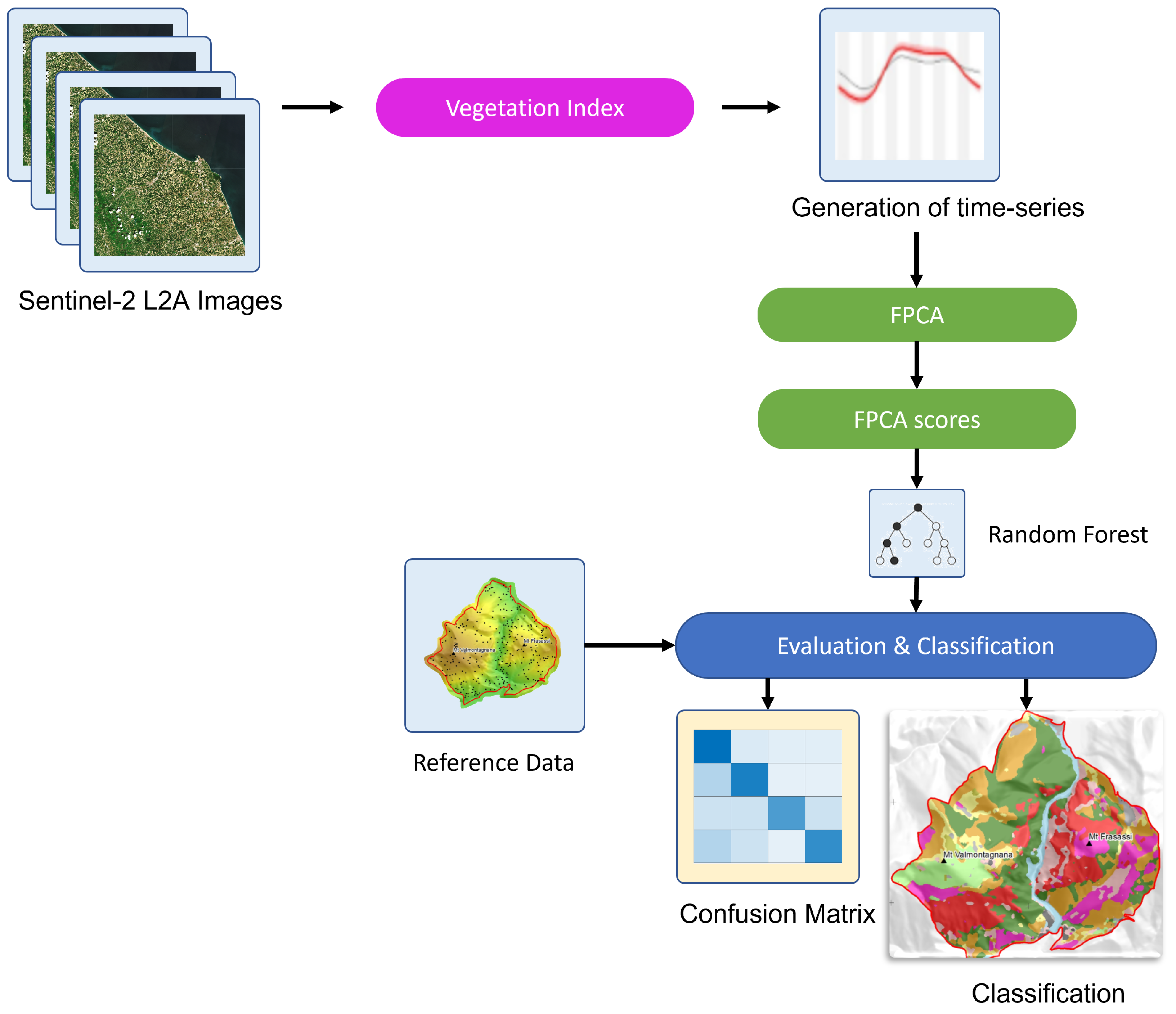
2.4. Remote Sensing Time-Series

L2A Sentinel-2 images were collected using the Sen2r [51] package. We considered scenes (from April 2017 to April 2020) with a cloud cover in the areas of interest lower than 25%. The clouds were masked and the images co-registered. A spatial resolution of 20 m was used; this value is suitable for forest plant communities studies (in our case, forests had almost full-coverage of the study area). The four spectral bands at 10 m (blue B2: 497 nm, green B3: 560 nm, red B4: 664 nm, and infrared B8: 835 nm) were re-sampled to 20 m. We obtained a stack of 93 Sentinel-2 pre-processed, co-registered images with 20 m spatial resolution.

We considered a set of vegetation indexes (see

Table 3. Vegetation indices applied to the time-series image stacks.

Vegetation Index	Acronym	References
Normalized Difference Vegetation Index	NDVI	[52]
Green Normalized Difference Vegetation Index	GNDVI	[53,54]
Modified Chlorophyll Absorption in Reflectance Index	MCARI	[55]
Normalized Difference Red-Edge	NDRE	[56]
Normalized Difference Water Index	NDWI	[57]
Modified Normalized Difference Water Index	MNDWI	[58]

) to capture seasonal variation in the VIS-NIR range. The selected (six) vegetation indexes were applied to the 93 images stack obtaining a data-cube (6 × 93).

Table A2. Distribution of selected Sentinel-2 images, by month.

Month	Frequency
January	4
February	8
March	7
April	7
May	8
June	9
July	12
August	14
September	9
October	7
November	3
December	5
sum	93

and

Table A3. List of Sentinel-2 images selected for this study.

Num	Date	Doy	Month	Num	Date	Doy	Month
1	21 April 2017	111	4	48	3 October 2018	276	10
2	1 May 2017	121	5	49	13 October 2018	286	10
3	11 May 2017	131	5	50	12 November 2018	316	11
4	31 May 2017	151	5	51	7 December 2018	341	12
5	20 June 2017	171	6	52	12 December 2018	346	12
6	10 July 2017	191	7	53	27 December 2018	361	12
7	20 July 2017	201	7	54	26 January 2019	26	1
8	30 July 2017	211	7	55	5 February 2019	36	2
9	9 August 2017	221	8	56	15 February 2019	46	2
10	19 August 2017	231	8	57	20 February 2019	51	2
11	29 August 2017	241	8	58	25 February 2019	56	2
12	18 September 2017	261	9	59	2 March 2019	61	3
13	8 October 2017	281	10	60	12 March 2019	71	3
14	18 October 2017	291	10	61	17 March 2019	76	3
15	28 October 2017	301	10	62	22 March 2019	81	3
16	27 November 2017	331	11	63	1 April 2019	91	4
17	7 December 2017	341	12	64	16 April 2019	106	4
18	22 December 2017	356	12	65	31 May 2019	151	5
19	6 January 2018	6	1	66	5 June 2019	156	6
20	15 February 2018	46	2	67	15 June 2019	166	6
21	6 April 2018	96	4	68	25 June 2019	176	6
22	16 April 2018	106	4	69	30 June 2019	181	6
23	21 April 2018	111	4	70	5 July 2019	186	7
24	26 April 2018	116	4	71	20 July 2019	201	7
25	11 May 2018	131	5	72	25 July 2019	206	7
26	16 May 2018	136	5	73	30 July 2019	211	7
27	21 May 2018	141	5	74	4 August 2019	216	8
28	31 May 2018	151	5	75	9 August 2019	221	8
29	10 June 2018	161	6	76	14 August 2019	226	8
30	15 June 2018	166	6	77	19 August 2019	231	8
31	20 June 2018	171	6	78	24 August 2019	236	8
32	30 June 2018	181	6	79	29 August 2019	241	8
33	10 July 2018	191	7	80	8 September 2019	251	9
34	15 July 2018	196	7	81	13 September 2019	256	9
35	20 July 2018	201	7	82	18 September 2019	261	9
36	25 July 2018	206	7	83	8 October 2019	281	10
37	30 July 2018	211	7	84	23 October 2019	296	10
38	4 August 2018	216	8	85	7 November 2019	311	11
39	9 August 2018	221	8	86	1 January 2020	1	1
40	19 August 2018	231	8	87	6 January 2020	6	1
41	24 August 2018	236	8	88	5 February 2020	36	2
42	29 August 2018	241	8	89	15 February 2020	46	2
43	3 September 2018	246	9	90	20 February 2020	51	2
44	8 September 2018	251	9	91	11 March 2020	71	3
45	18 September 2018	261	9	92	16 March 2020	76	3
46	23 September 2018	266	9	93	21 March 2020	81	3
47	28 September 2018	271	9

summarize the list of distributions and the list of the Sentinel-2 selected images for this study.

The collected scenes cover a multi-year period. We grouped/sorted them by their Day of the Year (DoY) to derive a dense annual time-series (e.g., [59,60]). We identified and removed the outlier values (function clean.ts() of the R package “forecast”; [61,62]) for each pixel, and then we aggregated (average) the DoY values in weekly values (1–52). We applied the Generalized Additive Model (GAM) [32] to smooth data obtaining a cubic spline representation of the pixel based time-series. We finally obtained six stack (vegetation indexes) of 52 rasters (weeks) that represent the spectra of all pixels over a year (Figure A2). The six time-series generated were then used to feed the FPCA analysis to enable classification using the FPCA scores.

Functional Principal Component Analysis (FPCA)

Functional Data Analysis (FDA) considers data as continuous functions. Therefore, each single pixel-based time-series was considered as a single entity (i.e., continuous function), rather than a mere sequence of discrete observations (e.g., a vector with 52 values as the number of weeks in a year).

Considering that the entire time-series of a pixel is a statistical unit, FPCA treats the entire raster stack (data cube) as a single object, consisting essentially of as many functions (trajectories of variation over time) as there are pixels in the study area. As in PCA, FPCA compresses information on an ortho-normal basis. The main difference is the capability of preserving the functional structure (i.e., the chronological order, in our case) of the analyzed data [33]. FPCA, similarly to PCA, provides eigenvalues that describe the variation explained by each component. The FPCA scores quantify the similarities between the functions (time-series based on pixels), while the eigenfunctions represent the main modes of variation of the data.

FPCA scores are a core aspect of this study, as they can be used in subsequent analyses (e.g., correlation analysis, functional data clustering [63], and supervised classification [35]). Using FPCA scores, it is possible to generate a reduced space where the functions (here, pixel-based time-series) can be plotted in an ordered way, thus, supporting domain experts in ecological interpretation [31]. The scores could be also used to fit the plant association seasonal temporal profiles (curves); in particular, in this study, we used the CreatePathPlot() function of the fdapace package [64] for this purpose.

This package was also used to perform six distinct FPCAs, one for each pixel-based vegetation index time-series. The pixel-based time-series were decomposed into their main variation modes over the year (FPCA components), and the related scores (i.e., pixel-based FPCA scores) were obtained. The FPCA scores were then used as inputs (predictors) to create plant associations and habitat models using a supervised algorithm (i.e., Random Forest).

2.5. Supervised Mapping Using Random Forest

RF is an ensemble learning classifier [65] that is often used in habitat mapping studies based on remote sensing. Belgiu and Drăguţ [66] presented a detailed review of RF and its efficiency in remote sensing. In RF, it is necessary to adjust certain parameters and aspects, such as: (i) the number of trees (the ntree parameter) that will be created by randomly selecting the samples from the training samples and (ii) the number of variables used for the division of the tree nodes (the mtry parameter).

We set ntree to 1500 and evaluated mtry from 1 to the square root of the number of input variables, as is typically done [66]. An RF can be biased if the proportions of training and validation data are unbalanced (as was the case in this study; see Table 1). This aspect could present issues and could lead to over-prediction of the majority classes and under-prediction of the minority classes. Over- and under-sampling can be used to produce more balanced data sets [67].

In order to make the frequency of the majority class closer to that of the rarest class, we incorporated down-sampling in the RF, when evaluating the training data subset (subset parameter). We set subset = 11 * nmin, where 11 is the number of target classes and nmin is the minimum between target classes (Table 1). This means that the RF model with ntree = 1500 can obtain a balanced random sample without a loss of information for the majority classes.

We considered two main groups of features:

• pixel-based FPCA scores, representing the main seasonal (intra-annual) variations of the time-series;
• pixel-based PCA scores, representing the topographic and lithological features.

RF models were constructed using the predictors both individually and jointly in order to evaluate and compare their contributions to the final accuracy of the map. We preliminarily applied Recursive Feature Elimination (RFE) to consider only the most discriminating predictors and reduce the (possibly high) number of dimensions. Mappings based on random forest models and accuracies were performed and assessed using the packages raster [68] and caret [69].

2.6. Classification and Mapping Accuracy Assessment

The mapping accuracy (classification) was evaluated using the Overall Accuracy (OA), Producer Accuracy (PA), and User Accuracy (UA) metrics [70], as well as the $\kappa$ coefficient [71]. We executed 10-fold cross-validation five times in order to calibrate the model and provide a robust estimate of the accuracy, thus limiting any potential bias. We provide the mean OA and $\kappa$ index (and their respective Standard Deviations) and a cross-validated confusion matrix (representing the error distribution for class among the five repeats).

We also performed a comparison between the reference data and a 1:10,000 scale vegetation map. The previous map was derived from acquisitions performed in 2009 and published online on a webGIS platform in 2014 (SIT-REM webGIS available here: http://sitbiodiversita.ambiente.marche.it/sitrem/, accessedon 10 February 2022) [72]. The types of vegetation and habitats between the different maps were appropriately harmonized (in terms of classes). We tested the matching between the maps and defined the respective levels of agreement through the $\kappa$ statistics.

3. Results

3.1. Main Seasonal Variations of Time-Series

FPCA was used to extract the orthogonal main modes of variation (FPCA components) from the multi-index Sentinel-2 time-series. Figure A1 shows the number of identified functional components (eight for the MCARI time-series and seven for all of the other time-series) and their fraction of variation explained (i.e., eigenvalues). FPCA components, in practice, represent the amount of deviation from the overall mean of the time-series, thus, reflecting the main contrasting modes of variation throughout the year.

In all of the considered cases, the two first FPCA components explained about 90% of the total variation (NDVI: FPCA1 66.40%, FPCA2 24.53%; NDWI: FPCA1 66.57%, FPCA2 24.26%; GNDVI: FPCA1 71.42%; FPCA2 18.76%; MNDWI: FPCA1 74.62%, FPCA2 16.01%; NDRE: FPCA1 60.97%, FPCA2 29.04%; and MCARI: FPCA1 56.31%, 26.54%) (Figure A1).

Figure A2 shows the temporal and spatial patterns of the two first FPCA components extracted from the 18,631 weekly pixel-based time-series (we considered all of the pixels belonging to the study area), while Figure A3 shows the mean seasonal profiles of plant associations and habitats. These profiles describe, in a compact and easily readable manner, the distinct phenological behaviors in relation to the different vegetation indices presented in this work (see Table 3).

3.2. Plant Community Modeling Using the Main Topographic–Lithological and Phenological Predictors

In this sub-section, we provide results from the RF models performed using both individual and joint predictors, where the pixel-based FPCA scores summarize the main seasonal (i.e., intra-annual) multi-spectral variations, while the pixel-based PCA scores summarize the topographic and lithological predictors.

Table A1. Comparison of performance (OA, K, UA, and PA) between traditional map (a) and models based on components: (b) topography, (c) NDVI, (d) GNDVI, (e) MCARI, (f) NDRE, (g) NDWI, (h) MNDWI, (i) all time-series, and (l) all time-series + topography. Legend numbers correspond to plant associations and habitats listed in Table 1.

	a	b	c	d	e	f	g	h	i	l
OA	59.4	59.2	73.1	69.5	63.7	69.5	67.9	67.3	82.1	85.5
		8.3	7.2	7.6	7.2	8.7	7.1	7.6	6.3	5.2
K	0.54	0.53	0.69	0.65	0.58	0.65	0.63	0.62	0.79	0.83
		0.09	0.08	0.08	0.08	0.10	0.08	0.08	0.07	0.06
PA
1	43.2	70.3	86.5	78.4	67.6	81.1	81.1	73.0	91.9	91.9
2	44.1	38.2	79.4	76.5	64.7	79.4	70.6	64.7	79.4	85.3
3	56.7	56.7	58.3	71.7	60.0	56.7	46.7	68.3	65.0	68.3
4	90.6	37.5	78.1	62.5	59.4	84.4	78.1	84.4	90.6	90.6
5	87.5	93.8	56.3	87.5	62.5	68.8	68.8	56.3	87.5	100.0
6	37.5	50.0	75.0	68.8	37.5	68.8	68.8	68.8	68.8	81.3
7	80.0	93.3	80.0	80.0	86.7	86.7	73.3	80.0	93.3	93.3
8	93.8	62.5	81.3	81.3	75.0	68.8	81.3	75.0	81.3	87.5
9	36.7	53.1	69.4	63.3	55.1	65.3	55.1	51.0	77.6	87.8
10	72.2	61.1	66.7	61.1	72.2	66.7	72.2	66.7	72.2	72.2
11	73.3	80.0	80.0	73.3	80.0	86.7	86.7	60.0	80.0	86.7
UA
1	47.1	68.4	78.0	72.5	64.1	83.3	85.7	64.3	82.9	85.0
2	36.6	44.8	57.4	68.4	47.8	57.4	49.0	51.2	60.0	65.9
3	57.6	64.2	79.5	86.0	75.0	82.9	68.3	77.4	83.0	85.4
4	63.0	44.4	75.8	60.6	57.6	71.1	78.1	84.4	90.6	90.6
5	100.0	75.0	60.0	87.5	47.6	68.8	37.9	60.0	77.8	88.9
6	40.0	42.1	57.1	45.8	35.3	45.8	68.8	61.1	64.7	76.5
7	100.0	66.7	52.2	60.0	68.4	61.9	47.8	66.7	70.0	87.5
8	55.6	43.5	76.5	86.7	85.7	78.6	81.3	75.0	81.3	82.4
9	78.3	65.0	91.9	86.1	71.1	84.2	87.1	71.4	88.4	93.5
10	50.0	61.1	85.7	64.7	86.7	75.0	65.0	63.2	100.0	92.9
11	100.0	60.0	75.0	57.9	66.7	76.5	81.3	52.9	75.0	81.3

summarizes the global, producer, and user accuracies.

The RF model based solely on topographical predictors achieved an overall accuracy of 59.25% ($\pm 8.32$) with k = 0.53 ($\pm 0.09$). Only Riparian woods, Juniperus oxycedrus shrubs, and Urban land achieved producer accuracies above 80%. All others showed very low performance (see Table A1). This demonstrates that it is necessary to consider and integrate different predictors.

In particular, as introduced in the previous sections, we evaluated several vegetation indices that have been widely used in related works. Each model (ranging from b to h) in Table A1) highlights the different behaviors for each class, mainly related to a certain vegetation index. The NDVI index for a given class performed better than other vegetation indices (e.g., class 4 NDVI and GNDVI).

However, when combining all time-series while also including the topography, the overall accuracy reached 85.5%—also showing optimal performances in terms of UA and PA. This suggests that each vegetation index contributes in a different (mostly constructive) way to accurately and precisely predict the target class, while non-radiometric features, such as the topographic and lithological predictors, also contributed to the overall performance (see columns i and l of Table A1).

3.3. Comparison of Obtained Results with Ancillary Data

As mentioned in the previous section, we also performed a comparison with an existing map (Figure 3b). The latest official map (produced by an expert through photo-interpretation) [72], compared with the reference data, showed an OA of 59.42% and k = 0.54. The best PAs were those of the Bromus erectus Huds. grasslands, the riparian woods, the Pinus sp. plantations, and the Juniperus oxycedrus shrubs, while various classes were less than 60% (e.g., Holm-oak, Downy-oak, and black hornbeam woods; see Table A1).

Both maps showed a similar trend over large areas, even if the supervised approach (Figure 3a) was able to output a more accurate map. Changes over time were negligible, considering that the intrinsic dynamics are significantly slower than the span of time between the construction of the SIT-REM maps [72] and that in this work.

4. Discussion

1.

Main results. Our results confirmed that remotely sensed data can be used to (automatically) map plant associations and habitats, particularly due to their multi-spectral seasonal profiles (phenological behaviors). The main seasonal multi-spectral variations were effective predictors for the production of accurate maps as previously discussed in [16,37].

In particular, the main seasonal variations extracted from Sentinel-2 time-series data using FPCA, according to the methodology proposed in Pesaresi et al. [37], proved to be an effective tool for mapping several plant associations (of different structure and specific composition) for an entire SAC. We used supervised random forest classification, similarly to Zhu and Liu [29,73,74,75], and revealed that the main spectral (phenological) seasonal variations contributed to the OA (here, 85.58%) of the produced map, much more strongly than the lithological and topographic features (see Table A1).

2.

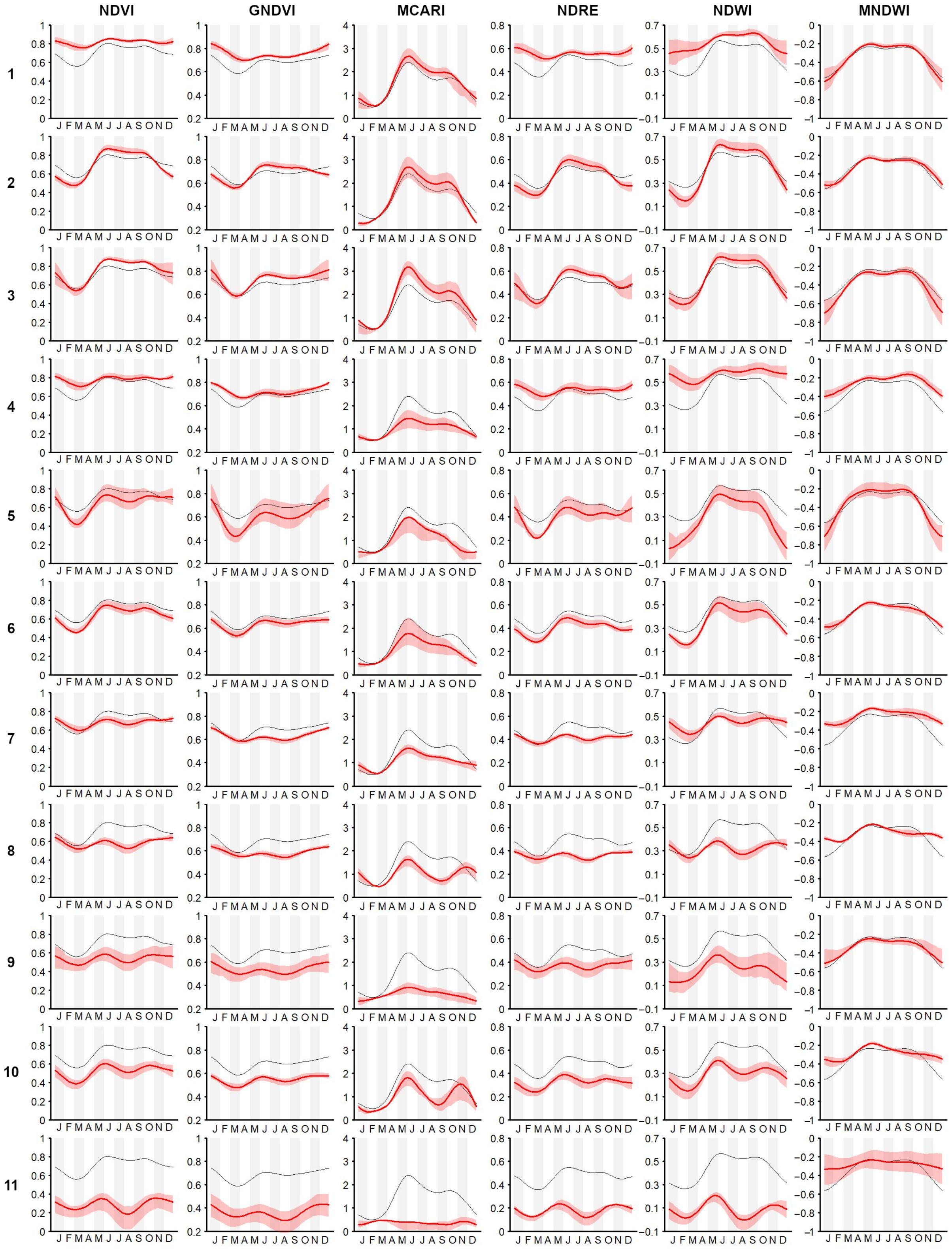
Simultaneous use of multiple time-series We confirmed the importance of using the popular NDVI time-series [76]. It was demonstrated (as in other related works, e.g., [8,24,75]) that the integration of multi-spectral (vegetation index) time-series can improve the performance of vegetation and habitat mapping, as seasonal patterns manifest differently in different spectral bands and vegetation indices [28] (Figure A3).

For example, holm-oak wood and Pinus sp. plantations had similar seasonal temporal profiles, in terms of the NDVI, while presenting clearly different MCARI profiles (Figure A3). The supervised RF models constructed using the time-series individually revealed that, for the study area, seasonal variations of the NDVI time-series were the most explanatory (OA 73.13% alone), while RF model constructed using the time-series jointly revealed some complementarity between the time-series, where each appeared to be useful in classifying different plant associations.

The integration of all six considered spectral vegetation indices supplied the RF with crucial variations characterizing and discriminating the different plant associations. With the combined model, an improvement of 9% in the OA over the best single time-series was obtained. When we also considered the topographic and lithological features, an additional 3.4% improvement was achieved (Table A1).

3.

Mapping accuracy The obtained results, in terms of the OA (85.58%), demonstrated a meaningful gain of performance when compared with the existing map [72]. Habitat (92/43/EEC) and plant association maps (using the Braun–Blanquet approach) rarely reach an overall accuracy greater than 80% [17]. In most cases, the number of classes is up to five [11,14,37,77,78,79,80], while an increase in the number of classes typically has a negative impact on the overall performance, reaching values close to 75%, as in [9,16,80,81,82,83,84].

From a methodological point of view, it is necessary to define an acceptable level of accuracy of a map generated using remotely sensed data [85,86], taking into consideration the related use-cases and scenarios. Although it is challenging to define a minimum value threshold for the mapping of plant communities and habitats, according to the above-mentioned references, we could consider that, with a number of target classes greater than five, an OA value of 80% represents a good result, while the range of 75–80% could be sufficient. When the number of classes is ≤5, a good result should exceed 85% OA, and it can be considered satisfactory if it exceeds the 80%.

4.

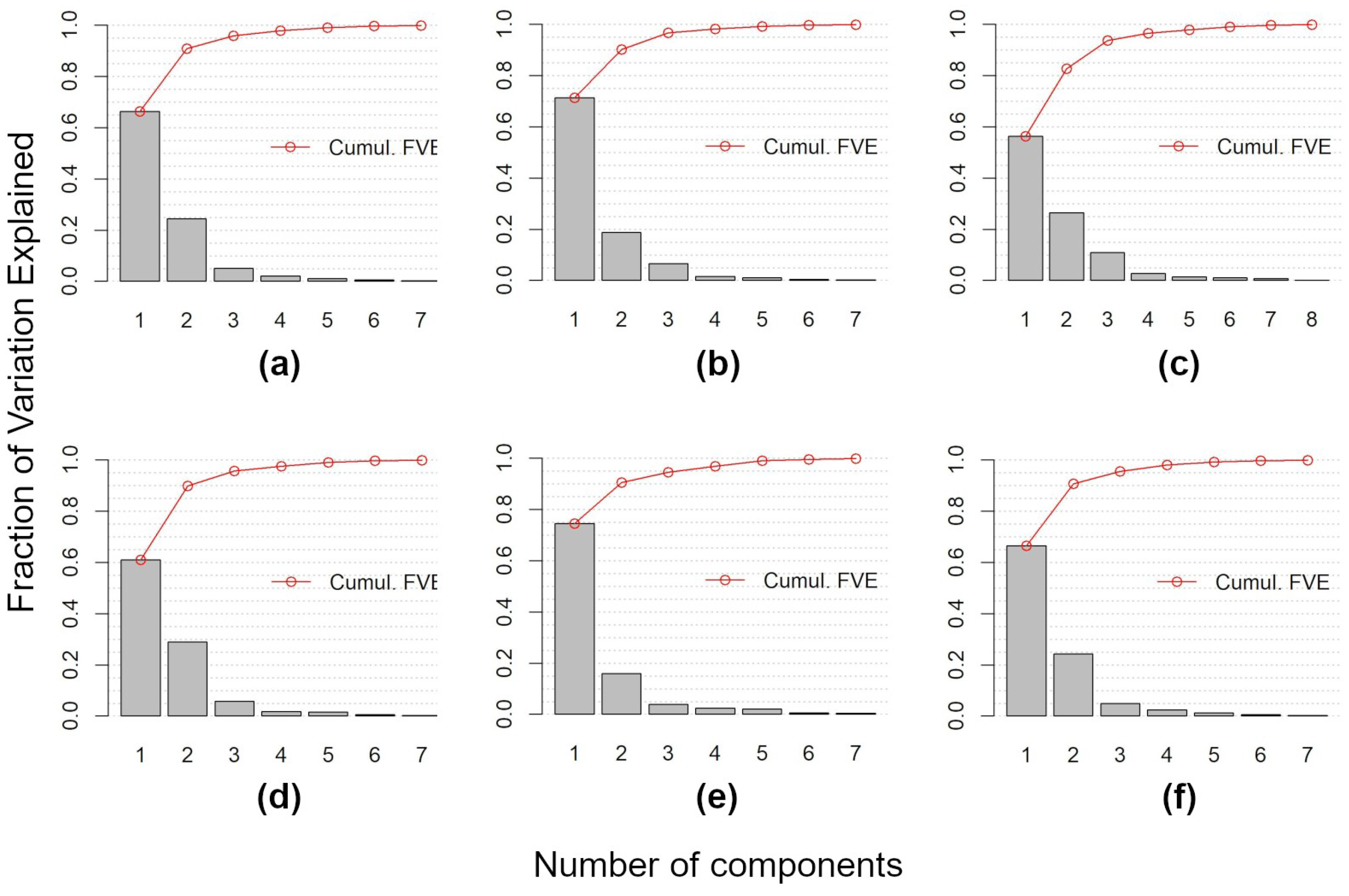
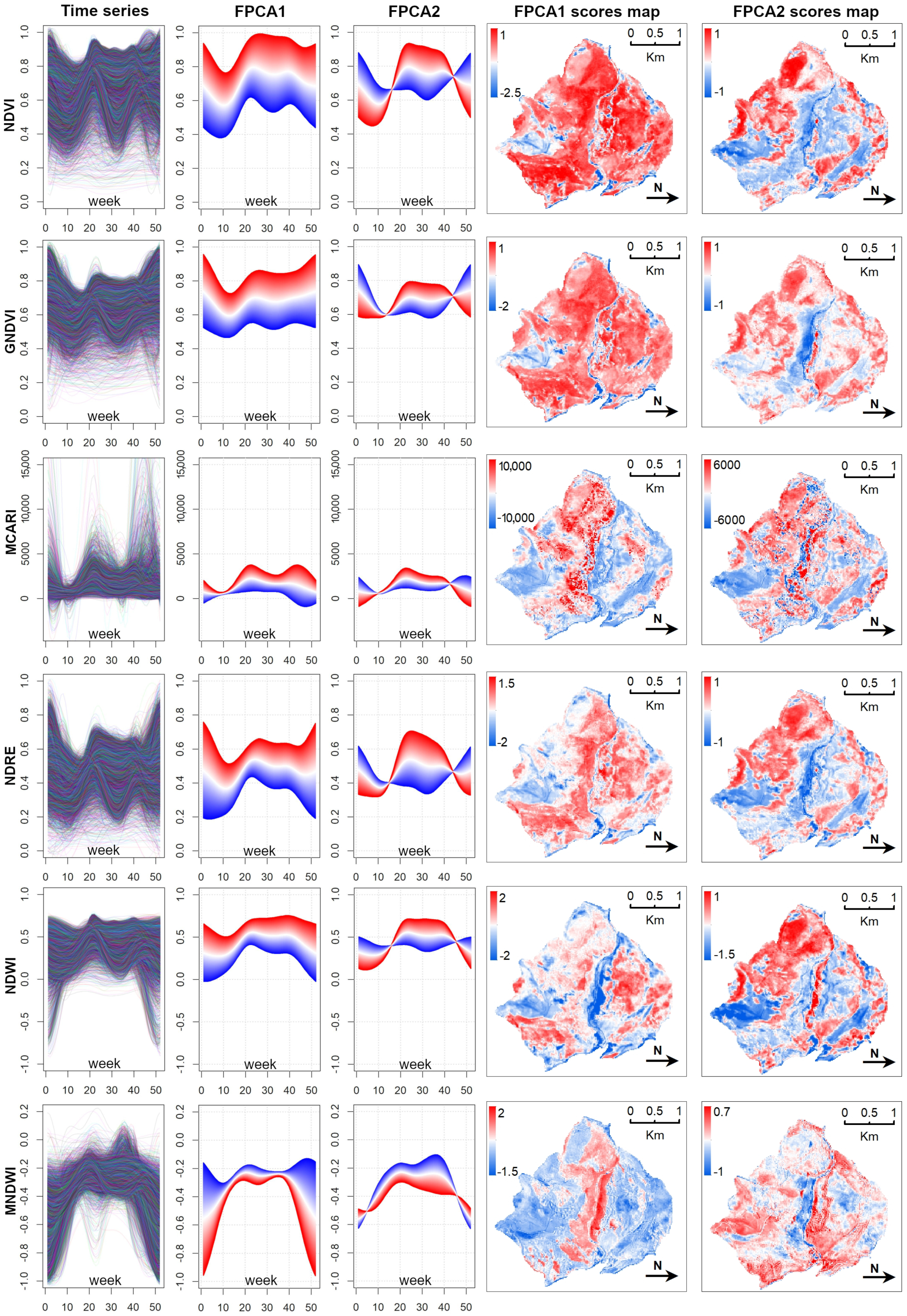
Data Reduction using FPCA FPCA is an efficient input data reduction tool. First, it is the central idea of the FDA itself—compressing the input data. Indeed, it considers the pixel-based time-series as a function and as the (unique) object of analysis. Consequently, FPCA considers a stack of remote sensed images as a single container of pixel-based functions, regardless of the number of images that compose it.

Then, FPCA extracts, from these pixel-based functions (considered as cohesive temporal record of pixel-based time-series), the main and orthogonal modalities of variation (i.e., functional components, numerically represented by the FPC scores that express the different seasonalities), preserving the order (i.e., chronology) of the data and facilitating ecological interpretation of the derived temporal and spatial patterns (see Figure A2; as well as [31,36,37]).

In this work, for each vegetation index, we derived the time-series (set of values over 52 weeks) and then applied FPCA. This technique reduced the size to a total of 43 functional components (considering multi-spectral seasonality); see Figure A1 and Figure A2.

Furthermore, functional analysis allows for the study of derivatives, thus, providing complementary information to describe the seasonal cycles derived from satellite data (see, e.g., [87,88]). The FPCA components with a low fraction of variance explained could also be evaluated by experts in order to derive local changes that are potential indicators of different plant communities [89].

5.

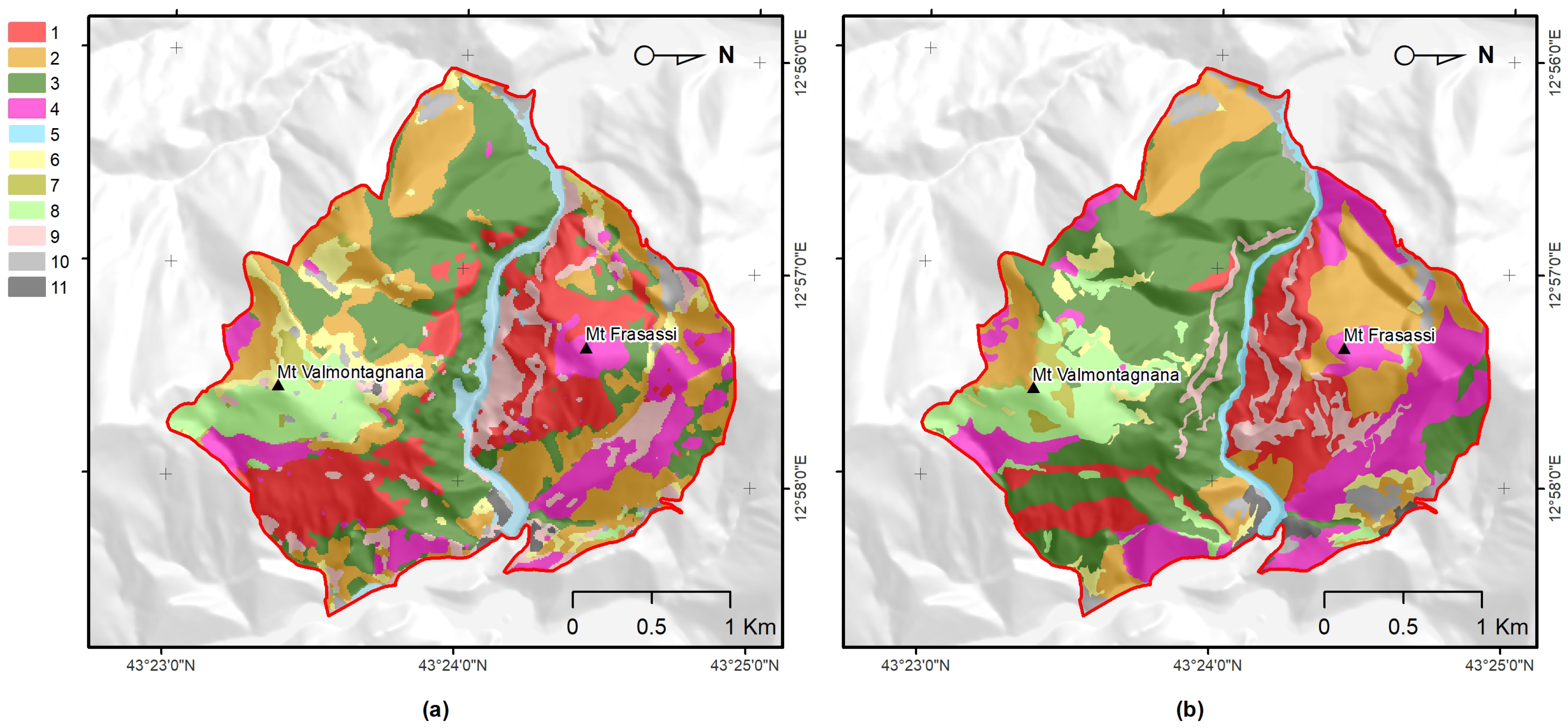
Benefits for habitat directives, phyto-sociology, and landscape management The overall accuracy obtained (OA 85.58%) was greater than 80% and much higher than that obtained with the traditional method (photo-interpretation), thus, making the produced map (Figure 3) a reliable and usable tool in the main procedures of habitat directives (e.g., Appropriate Assessments and filling in of Standard Data Forms).

In the study area, the high temporal resolution of the Sentinel-2 mission makes mapping (through the functional approach) of the vegetation and habitats up-to-date and repeatable, according to the timing required by the directive (six years), as well as with higher frequencies (e.g., every 2–3 years) [9]. Cyclical mapping (at least every six years, in accordance with the Habitats Directive) of the plant associations—and, therefore, of the habitats—with high accuracy (in terms of OA) could provide a valid tool for monitoring the transformation of habitats over time [10,90].

For example, the conservation status of the grasslands in the studied area is strongly determined by the presence of invasive shrubs or species. The grasslands of habitat 6210, in fact, if not adequately managed, tend to be colonized by shrubs (e.g., Spartium junceum and Juniperus oxycedrus) and by a few perennial grasses, such as those of the genera Brachypodium, with a consequent loss of the floristic diversity of the grasslands [91,92,93,94].

Any variation or modification of the phenological profile of the habitat (as identifiable through the use of the proposed methodology) can be used as a warning signal that, in certain areas, a transformation process is underway, therefore, highlighting the need for an inspection on the ground and, consequently, the need for corrective and timely management actions.

The limitation for modeling and mapping plant communities is no longer the access and processing of satellite data, but rather the time it takes to access and generate reference data in the field. Therefore, it is crucial to disseminate the vegetation plots in databases (e.g., VegItaly [95]) [9]. The production of reference data at the plant associations level could benefit from the help of drones. An unmanned aerial vehicle could enable the recognition of the plant species (see, e.g., [96]) while reaching inaccessible places for human beings due to orography and many other factors.

Recognizing few indicator species (by drone) could by key for the quick identification of vegetation types (plant association) in the field in complex environments [97] where the vegetation types and their species composition are available. Despite the high global accuracy of the map, the error matrix (

Table 4. Cross-validated confusion matrix (10-fold, repeated five times) between the predicted target classes of the SAC “Gola di Frasassi”, code IT5320003 (Central Italy). The Overall accuracy, Producer accuracy, User accuracy (in percentage), and $\kappa$ Statistic are given. Row and column numbers denote the plant associations and habitats listed in Table 1.

		Reference Data
		1	2	3	4	5	6	7	8	9	10	11	UA
Prediction	1	34	0	5	1	0	0	0	0	0	0	0	85.0
	2	0	29	12	0	0	2	0	0	1	0	0	65.9
	3	1	4	41	1	0	0	0	0	0	0	1	85.4
	4	2	0	1	29	0	0	0	0	0	0	0	90.6
	5	0	0	1	0	16	0	0	0	0	1	0	88.9
	6	0	0	0	0	0	13	0	1	1	2	0	76.5
	7	0	0	0	1	0	1	14	0	0	0	0	87.5
	8	0	0	0	0	0	0	1	14	1	1	0	82.4
	9	0	1	0	0	0	0	0	0	43	1	1	93.5
	10	0	0	0	0	0	0	0	1	0	13	0	92.9
	11	0	0	0	0	0	0	0	0	3	0	13	81.3
	PA	91.9	82.5	68.3	90.6	100.0	81.3	93.3	87.5	87.8	72.2	86.7
	OA	85.58 (±5.28)
	K	0.83 (±0.06)

) showed that black hornbeam wood and downy-oak wood (habitat 91AA*) could be misclassified.

This was due to the fact that both woods share some species in the dominant tree layer, although the underlying, dominated layers are well-differentiated, in terms of mesophilic species dominating in the first case, with more thermophilic in the second. Therefore, from an ecological point of view, they are different woods, even if the tree structure and composition is partially similar. This confusion led to over-representation of downy-oak wood (PA 82.5% and UA of 65.9%) and under-representation of black hornbeam wood (PA 68.3% and UA 85.4%) in the predicted map (Figure 3). However, these accuracies were still much better than those obtained with traditional mapping.

The methodology presented in this work enables a concrete link between the remote survey perspective and the (phyto-sociological) field-based one. Manual (traditional) approaches could be empowered by supervised ones, which, in any case, still rely on reference data generated by domain experts.

Vegetation has unique spectral signatures that evolve along with the plant life cycle over the year [75], which represents an important trait of plant associations (Figure A3). The quantification of patterns in the seasonal behavior of the spectral reflectance can provide better characterization of plant communities [74]. Furthermore, FPCA scores represent reduced ordination spaces (i.e., useful tools for botanists and ecologists) [31,35,36] that are suitable for the ecological interpretation of the results and that contribute to the study of the relationships between the data observed in the field and those that are remotely sensed.

Limits and Challenges for Future Work

1.

We found that the combined use of different spectral vegetation indices led to better results compared with using a single one. Of course, the six selected vegetation indices have been widely adopted by researchers; however, we cannot exclude that a different set of vegetation indices combining two or more bands could improve the overall performance, perhaps also fixing the misclassification between black hornbeam and downy-oak woods. The typical formula adopted for the NDVI is in the form of $\left(a-b\right)/\left(a+b\right)$ where a and b are spectral bands; this formula is only an example, and other formulas/functions may improve the final mapping.

2.

If we need to consider multiple time-series derived from a wider set of vegetation indices, we must adapt an approach considering more advanced FDA techniques. A possible solution is to adopt the Multidimensional FPCA (MFPCA) [98], which enables reduction of the time-series (i.e., a lower number of components extracted from multiple time-series), thus, providing a single phenological ordering space to make the ecological interpretation easier [37]. Although harmonic and phenological features have recently been used to improve forest type mapping, as in [29,74], new vegetation indices could be derived, with novel formulas, in order to increase the spectral separation among target classes.

5. Conclusions

Functional Data Analysis (FDA) (e.g., FPCA) is relatively recent and not yet widely used in remote sensing and ecology, even if it represents a powerful way to analyze temporal ecological data, such as remote-sensing time series [99]. FDA represents a promising novelty to map habitats that belong to the Natura 2000 network sites. Pesaresi et al. [36,37] applied the FPCA to NDVI Landsat 8 time-series to map and characterize forest plant associations and habitats identified with the phytosociological approach in a small area belonging to the Natura 2000 network.

In this work, we demonstrated the utility of using FPCA applied to Sentinel-2 time series of vegetation indexes to improve the mapping of plant associations and habitats of an entire Special Area of Conservation. Despite its limited size (∼728 ha), the study area is rich in terms of species, plant communities and habitat diversity.

The global accuracy achieved in the study area adopting the proposed methodology was 85.58%. The obtained results outperformed the threshold of the 80% that was rarely exceeded in remote sensing applications for habitat mapping and the existing map of the same area that was obtained by experts using photointerpretation. The main seasonal phenological variations (FPCA components and scores), extracted by FPCA from the remote sensed time series, contributed to the global accuracy of the map much more than the topographic and lithological variables.

Furthermore, this work highlighted that the plant communities, together with their own typical floristic composition, exhibited exclusive phenological dynamics that manifest differently with respect to vegetation indexes. These different temporal patterns are quantified by FPCA scores and graphically represented by their mean seasonal profiles. The proposed methodology can be used to detect future changes in phenological patterns that can serve as a warning sign of habitat change. Indeed, they act as a sensible and pragmatic tool to show, monitor, and preview environmental changes.

FPCA scores and multi-index mean seasonal profiles are important vegetation attributes that could be complementary to species-based approaches in plant community ecology and phytosociolocy and that facilitate the link between remote sensing with habitat mapping and monitoring and their ecological interpretation.

The results confirm that FDA applied to remote-sensing times-series opens new scenarios to map vegetation and habitats of the Natura 2000 network. Vegetation and habitat mapping are still mostly performed in the traditional way with the photo-interpretation method. Most of approaches to map habitat from remotely sensed data rely on single or sparse time-series (few images per year); however, the dynamics of phenology suggest using denser time series to set up a supervised classifier (Random Forest, LDA, SVM, etc.).

The FDA techniques, considering the time series of a pixel as a single statistical object (function) allow the use of many images (dense time-series) in an efficient and ecologically relevant way considering entire archives of remotely sensed images (e.g., Landsat and Sentinel-2) as a cohesive temporal record, rather than as a series of individual images.

Considering these results, we plan to extend the temporal coverage of time-series embedding different combinations of bands (indexes) that could improve the overall classification performance in a multi-dimensional scenario by using the Multivariate Functional Principal Component Analysis (MFPCA). The proposed method could be easily applied on different, larger areas with denser time-series.

We believe that the mapping of plant associations and habitats with the functional approach has a relevant impact on the decisions taken by policy makers to monitor and preserve our environments. The automation of the process also gives the opportunity to detect changes over time that could be relevant for stakeholders to plan and enact policies to preserve the environment.

References

- Braun–Blanquet, J.; Conard, H.S.; Fuller, G.D. Plant Sociology: The Study of Plant Communities, 1st ed.; McGraw-Hill: New York, NY, USA; London, UK, 1932; p. 439. [Google Scholar] [CrossRef] [Green Version]
- Chytrý, M.; Schaminée, J.H.J.; Schwabe, A. Vegetation survey: A new focus for Applied Vegetation Science. Appl. Veg. Sci. 2011, 14, 435–439. [Google Scholar] [CrossRef]
- Mucina, L. Europe, Ecosystems of. In Encyclopedia of Biodiversity, 2nd ed.; Levin, S.A., Ed.; Academic Press: Waltham, MA, USA, 2013; pp. 333–346. [Google Scholar] [CrossRef]
- Biondi, E. Phytosociology today: Methodological and conceptual evolution. Plant Biosyst. 2011, 145, 19–29. [Google Scholar] [CrossRef]
- Biondi, E.; Burrascano, S.; Casavecchia, S.; Copiz, R.; Del Vico, E.; Galdenzi, D.; Gigante, D.; Lasen, C.; Spampinato, G.; Venanzoni, R.; et al. Diagnosis and syntaxonomic interpretation of Annex I Habitats (Dir. 92/43/EEC) in Italy at the alliance level. Plant Sociol. 2012, 49, 5–37. [Google Scholar] [CrossRef]
- Rodwell, J.S.; Evans, D.; Schaminée, J.H. Phytosociological relationships in European Union policy-related habitat classifications. Rend. Lincei 2018, 29, 237–249. [Google Scholar] [CrossRef]
- CEC. Council Directive 92/43/EEC of 21 May 1992 on the conservation of natural habitats and of wild fauna and flora. Off. J. L 1992, 206, 7–50. [Google Scholar]
- Tarantino, C.; Forte, L.; Blonda, P.; Vicario, S.; Tomaselli, V.; Beierkuhnlein, C.; Adamo, M. Intra-annual sentinel-2 time-series supporting grassland habitat discrimination. Remote Sens. 2021, 13, 277. [Google Scholar] [CrossRef]
- Rapinel, S.; Rozo, C.; Delbosc, P.; Bioret, F.; Bouzillé, J.B.; Hubert-Moy, L. Contribution of free satellite time-series images to mapping plant communities in the Mediterranean Natura 2000 site: The example of Biguglia Pond in Corse (France). Mediterr. Bot. 2020, 41, 181–191. [Google Scholar] [CrossRef]
- Ichter, J.; Savio, L.; Evans, D.; Poncet, L. State-of-the-art of vegetation mapping in Europe: Results of a European survey and contribution to the French program CarHAB. Doc. Phytosociol. Ser. 3 2017, 6, 335–352. [Google Scholar]
- Feret, J.B.; Corbane, C.; Alleaume, S. Detecting the Phenology and Discriminating Mediterranean Natural Habitats with Multispectral Sensors-An Analysis Based on Multiseasonal Field Spectra. IEEE J. Sel. Top. Appl. Earth Obs. Remote Sens. 2015, 8, 2294–2305. [Google Scholar] [CrossRef]
- Corbane, C.; Güttler, F.; Alleaume, S.; Ienco, D.; Teisseire, M. Monitoring the phenology of mediterranean natural habitats with multispectral sensors—An analysis based on multiseasonal field spectra. In Proceedings of the 2014 IEEE Geoscience and Remote Sensing Symposium, Quebec City, QC, Canada, 13–18 July 2014; pp. 3934–3937. [Google Scholar] [CrossRef] [Green Version]
- Grignetti, A.; Salvatori, R.; Casacchia, R.; Manes, F. Mediterranean vegetation analysis by multi-temporal satellite sensor data. Int. J. Remote Sens. 1997, 18, 1307–1318. [Google Scholar] [CrossRef]
- Marzialetti, F.; Giulio, S.; Malavasi, M.; Sperandii, M.G.; Acosta, A.T.R.; Carranza, M.L. Capturing Coastal Dune Natural Vegetation Types Using a Phenology-Based Mapping Approach: The Potential of Sentinel-2. Remote Sens. 2019, 11, 1506. [Google Scholar] [CrossRef] [Green Version]
- Hoffmann, S.; Schmitt, T.M.; Chiarucci, A.; Irl, S.D.H.; Rocchini, D.; Vetaas, O.R.; Tanase, M.A.; Mermoz, S.; Bouvet, A.; Beierkuhnlein, C. Remote sensing of β-diversity: Evidence from plant communities in a semi-natural system. Appl. Veg. Sci. 2019, 22, 13–26. [Google Scholar] [CrossRef] [Green Version]
- Rapinel, S.; Mony, C.; Lecoq, L.; Clément, B.; Thomas, A.; Hubert-Moy, L. Evaluation of Sentinel-2 time-series for mapping floodplain grassland plant communities. Remote Sens. Environ. 2019, 223, 115–129. [Google Scholar] [CrossRef]
- Vanden Borre, J.; Paelinckx, D.; Mücher, C.A.; Kooistra, L.; Haest, B.; De Blust, G.; Schmidt, A.M. Integrating remote sensing in Natura 2000 habitat monitoring: Prospects on the way forward. J. Nat. Conserv. 2011, 19, 116–125. [Google Scholar] [CrossRef]
- Corbane, C.; Lang, S.; Pipkins, K.; Alleaume, S.; Deshayes, M.; García Millán, V.E.; Strasser, T.; Vanden Borre, J.; Toon, S.; Michael, F. Remote sensing for mapping natural habitats and their conservation status—New opportunities and challenges. Int. J. Appl. Earth Obs. Geoinf. 2015, 37, 7–16. [Google Scholar] [CrossRef]
- Cabello, J.; Mairota, P.; Alcaraz-Segura, D.; Arenas-Castro, S.; Escribano, P.; Leitão, P.J.; Martínez-López, J.; Regos, A.; Requena-Mullor, J.M. Satellite remote sensing of ecosystem functions: Opportunities and challenges for reporting obligations of the EU habitat directive. Int. Geosci. Remote Sens. Symp. 2018, 2018, 6604–6607. [Google Scholar] [CrossRef]
- Schmidt, J.; Fassnacht, F.E.; Förster, M.; Schmidtlein, S. Synergetic use of Sentinel-1 and Sentinel-2 for assessments of heathland conservation status. Remote Sens. Ecol. Conserv. 2018, 4, 225–239. [Google Scholar] [CrossRef] [Green Version]
- Marzialetti, F.; Di Febbraro, M.; Malavasi, M.; Giulio, S.; Acosta, A.T.R.; Carranza, M.L. Mapping Coastal Dune Landscape through Spectral Rao’s Q Temporal Diversity. Remote Sens. 2020, 12, 2315. [Google Scholar] [CrossRef]
- Stendardi, L.; Karlsen, S.R.; Niedrist, G.; Gerdol, R.; Zebisch, M.; Rossi, M.; Notarnicola, C. Exploiting time series of Sentinel-1 and Sentinel-2 imagery to detect meadow phenology in mountain regions. Remote Sens. 2019, 11, 542. [Google Scholar] [CrossRef] [Green Version]
- Bajocco, S.; Ferrara, C.; Alivernini, A.; Bascietto, M.; Ricotta, C. Remotely-sensed phenology of Italian forests: Going beyond the species. Int. J. Appl. Earth Obs. Geoinf. 2019, 74, 314–321. [Google Scholar] [CrossRef]
- Chignell, S.M.; Luizza, M.W.; Skach, S.; Young, N.E.; Evangelista, P.H. An integrative modeling approach to mapping wetlands and riparian areas in a heterogeneous Rocky Mountain watershed. Remote Sens. Ecol. Conserv. 2018, 4, 150–165. [Google Scholar] [CrossRef] [Green Version]
- Schmidt, T.; Schuster, C.; Kleinschmit, B.; Förster, M. Evaluating an intra-annual time series for grassland classification—How many acquisitions and what seasonal origin are optimal? IEEE J. Sel. Top. Appl. Earth Obs. Remote Sens. 2014, 7, 3428–3439. [Google Scholar] [CrossRef]
- Lopes, M.; Frison, P.L.; Durant, S.M.; Schulte to Bühne, H.; Ipavec, A.; Lapeyre, V.; Pettorelli, N. Combining optical and radar satellite image time series to map natural vegetation: Savannas as an example. Remote Sens. Ecol. Conserv. 2020, 6, 316–326. [Google Scholar] [CrossRef]
- Young, N.E.; Anderson, R.S.; Chignell, S.M.; Vorster, A.G.; Lawrence, R.; Evangelista, P.H. A survival guide to Landsat preprocessing. Ecology 2017, 98, 920–932. [Google Scholar] [CrossRef] [Green Version]
- Pasquarella, V.J.; Holden, C.E.; Kaufman, L.; Woodcock, C.E. From imagery to ecology: Leveraging time series of all available Landsat observations to map and monitor ecosystem state and dynamics. Remote Sens. Ecol. Conserv. 2016, 2, 152–170. [Google Scholar] [CrossRef]
- Adams, B.; Iverson, L.; Matthews, S.; Peters, M.; Prasad, A.; Hix, D.M. Mapping Forest Composition with Landsat Time Series: An Evaluation of Seasonal Composites and Harmonic Regression. Remote Sens. 2020, 12, 610. [Google Scholar] [CrossRef] [Green Version]
- Kennedy, R.E.; Andréfouët, S.; Cohen, W.B.; Gómez, C.; Griffiths, P.; Hais, M.; Healey, S.P.; Helmer, E.H.; Hostert, P.; Lyons, M.B.; et al. Bringing an ecological view of change to landsat-based remote sensing. Front. Ecol. Environ. 2014, 12, 339–346. [Google Scholar] [CrossRef]
- Hurley, M.A.; Hebblewhite, M.; Gaillard, J.; Dray, S.; Taylor, K.A.; Smith, W.K.; Zager, P.; Bonenfant, C. Functional analysis of normalized difference vegetation index curves reveals overwinter mule deer survival is driven by both spring and autumn phenology. Philos. Trans. R. Soc. Lond. Ser. B Biol. Sci. 2014, 369, 20130196. [Google Scholar] [CrossRef] [PubMed] [Green Version]
- Ramsay, J. Functional Data Analysis; John Wiley & Sons: Hoboken, NJ, USA, 2005. [Google Scholar] [CrossRef]
- Di Salvo, F.; Ruggieri, M.; Plaia, A. Functional principal component analysis for multivariate multidimensional environmental data. Environ. Ecol. Stat. 2015, 22, 739–757. [Google Scholar] [CrossRef]
- Shang, H.L. A survey of functional principal component analysis. Adv. Stat. Anal. 2014, 98, 121–142. [Google Scholar] [CrossRef] [Green Version]
- Li, H.; Xiao, G.; Xia, T.; Tang, Y.Y.; Li, L. Hyperspectral image classification using functional data analysis. IEEE Trans. Cybern. 2014, 44, 1544–1555. [Google Scholar] [CrossRef] [PubMed]
- Pesaresi, S.; Mancini, A.; Casavecchia, S. Recognition and Characterization of Forest Plant Communities through Remote-Sensing NDVI Time Series. Diversity 2020, 12, 313. [Google Scholar] [CrossRef]
- Pesaresi, S.; Mancini, A.; Quattrini, G.; Casavecchia, S. Mapping mediterranean forest plant associations and habitats with functional principal component analysis using Landsat 8 NDVI time series. Remote Sens. 2020, 12, 1132. [Google Scholar] [CrossRef] [Green Version]
- Rivas-Martínez, S.; Sáenz, S.R.; Penas, A. Worldwide bioclimatic classification system. Glob. Geobot. 2011, 1, 1–634. [Google Scholar]
- Pesaresi, S.; Biondi, E.; Casavecchia, S. Bioclimates of Italy. J. Maps 2017, 13, 955–960. [Google Scholar] [CrossRef]
- Biondi, E.; Casavecchia, S.; Gigante, D. Contribution to the syntaxonomic knowledge of the Quercus ilex L. woods of the Central European Mediterranean Basin. Fitosociologia 2003, 40, 129–156. [Google Scholar]
- Blasi, C.; Feoli, E.; Avena, G.C. Due nuove associazioni dei Quercetalia pubescentis dell’Appennino centrale. Stud. Geobot. 1982, 2, 155–167. [Google Scholar]
- Blasi, C.; Di Pietro, R.; Filesi, L. Syntaxonomical revision of Quercetalia pubescenti-petraeae in the Italian Peninsula. Fitosociologia 2004, 41, 87–164. [Google Scholar]
- Allegrezza, M.; Pesaresi, S.; Ballelli, S.; Tesei, G.; Ottaviani, C. Influences of mature pinus nigra plantations on the floristic-vegetational composition along an altitudinal gradient in the central apennines, Italy. IForest 2020, 13, 279–285. [Google Scholar] [CrossRef]
- Biondi, E.; Casavecchia, S. Inquadramento fitosociologico della vegetazione arbustiva di un settore dell’Appennino settentrionale. Fitosociologia 2002, 39, 65–73. [Google Scholar]
- Biondi, E.; Allegrezza, M.; Zuccarello, V. Syntaxonomic revision of the Apennine grasslands belonging to Brometalia erecti, and an analysis of their relationships with the xerophilous vegetation of Rosmarinetea officinalis (Italy). Phytocoenologia 2005, 35, 129–164. [Google Scholar] [CrossRef]
- Allegrezza, M.; Biondi, E.; Ballelli, S.; Formica, E. La vegetazione dei settori rupestri calcarei dell’Italia centrale. Fitosociologia 1997, 32, 91–120. [Google Scholar]
- Geobotanic Group at Università Politecnica delle Marche. Dataset and Code Related to the Habitat Mapping of SAC of Frasassi. Available online: https://github.com/geobotany/habitatmapfrasassi (accessed on 10 February 2022).
- Franklin, J. Predictive vegetation mapping: Geographic modelling of biospatial patterns in relation to environmental gradients. Prog. Phys. Geogr. Earth Environ. 1995, 19, 474–499. [Google Scholar] [CrossRef]
- Regione Marche. La Carta Geologica Della Regione Marche in Scala 1:10.000. 2001. Available online: http://www.regione.marche.it/Regione-Utile/Paesaggio-Territorio-Urbanistica/Cartografia/Repertorio/Cartageologicaregionale10000 (accessed on 10 February 2022).
- Dray, S.; Dufour, A.B. The ade4 Package: Implementing the Duality Diagram for Ecologists. J. Stat. Softw. 2007, 22, 1–20. [Google Scholar] [CrossRef] [Green Version]
- Ranghetti, L.; Boschetti, M.; Nutini, F.; Busetto, L. “sen2r”: An R toolbox for automatically downloading and preprocessing Sentinel-2 satellite data. Comput. Geosci. 2020, 139, 104473. [Google Scholar] [CrossRef]
- Rouse, J.W.; Haas, R.H.; Schell, J.A.; Deering, D.W. Monitoring vegetation systems in the Great Plains with ERTS 10–14 December. In Proceedings of the Third ERTS Symposium; NASA: Washington, DC, USA, 1973; pp. 309–317. [Google Scholar]
- Buschmann, C.; Nagel, E. In vivo spectroscopy and internal optics of leaves as basis for remote sensing of vegetation. Int. J. Remote Sens. 1993, 14, 711–722. [Google Scholar] [CrossRef]
- Gitelson, A.A.; Kaufman, Y.J.; Merzlyak, M.N. Use of a green channel in remote sensing of global vegetation from EOS-MODIS. Remote Sens. Environ. 1996, 58, 289–298. [Google Scholar] [CrossRef]
- Daughtry, C. Estimating Corn Leaf Chlorophyll Concentration from Leaf and Canopy Reflectance. Remote Sens. Environ. 2000, 74, 229–239. [Google Scholar] [CrossRef]
- Barnes, E.; Clarke, T.; Richards, S.; Colaizzi, P.; Haberland, J.; Kostrzewski, M.; Waller, P.; Choi, C.; Riley, E.; Thompson, T.; et al. Coincident detection of crop water stress, nitrogen status and canopy density using ground based multispectral data. In Proceedings of the Fifth International Conference on Precision Agriculture, Bloomington, MN, USA, 16–19 July 2000; Volume 1619. [Google Scholar]
- Gao, B.C. NDWI—A normalized difference water index for remote sensing of vegetation liquid water from space. Remote Sens. Environ. 1996, 58, 257–266. [Google Scholar] [CrossRef]
- Xu, H. Modification of normalised difference water index (NDWI) to enhance open water features in remotely sensed imagery. Int. J. Remote Sens. 2006, 27, 3025–3033. [Google Scholar] [CrossRef]
- Fisher, J.I.; Mustard, J.F.; Vadeboncoeur, M.A. Green leaf phenology at Landsat resolution: Scaling from the field to the satellite. Remote Sens. Environ. 2006, 100, 265–279. [Google Scholar] [CrossRef]
- Schuster, C.; Schmidt, T.; Conrad, C.; Kleinschmit, B.; Förster, M. Grassland habitat mapping by intra-annual time series analysis -Comparison of RapidEye and TerraSAR-X satellite data. Int. J. Appl. Earth Obs. Geoinf. 2015, 34, 25–34. [Google Scholar] [CrossRef]
- Hyndman, R.J.; Khandakar, Y. Automatic Time Series Forecasting: The forecast Package for R. J. Stat. Softw. 2008, 27, 1–22. [Google Scholar] [CrossRef] [Green Version]
- Hyndman, R.; Athanasopoulos, G.; Bergmeir, C.; Caceres, G.; Chhay, L.; O’Hara-Wild, M.; Petropoulos, F.; Razbash, S.; Wang, E.; Yasmeen, F. Forecast: Forecasting Functions for Time Series and Linear Models, R Package Version 8.15; 2021. Available online: https://pkg.robjhyndman.com/forecast/ (accessed on 10 February 2022).
- Jacques, J.; Preda, C. Functional data clustering: A survey. Adv. Data Anal. Classif. 2014, 8, 231–255. [Google Scholar] [CrossRef] [Green Version]
- Dai, X.; Hadjipantelis, P.Z.; Han, K.; Ji, H. Fdapace: Functional Data Analysis and Empirical Dynamics, R Package Version 0.4.0; 2018. Available online: https://CRAN.R-project.org/package=fdapace/ (accessed on 10 February 2022).
- Breiman, L. Random Forests. Mach. Learn. 2001, 45, 5–32. [Google Scholar] [CrossRef] [Green Version]
- Belgiu, M.; Drăguţ, L. Random forest in remote sensing: A review of applications and future directions. ISPRS J. Photogramm. Remote Sens. 2016, 114, 24–31. [Google Scholar] [CrossRef]
- Evans, J.S.; Cushman, S.A. Gradient modeling of conifer species using random forests. Landsc. Ecol. 2009, 24, 673–683. [Google Scholar] [CrossRef]
- Hijmans, R.J. Raster: Geographic Data Analysis and Modeling, R Package Version 2.8-4; 2018. Available online: https://CRAN.R-project.org/package=raster/ (accessed on 10 February 2022).
- Kuhn, M. Building Predictive Models in R Using the caret Package. J. Stat. Softw. Artic. 2008, 28, 1–26. [Google Scholar] [CrossRef] [Green Version]
- Congalton, R.G. A review of assessing the accuracy of classifications of remotely sensed data. Remote Sens. Environ. 1991, 37, 35–46. [Google Scholar] [CrossRef]
- Cohen, J. A Coefficient of Agreement for Nominal Scales. Educ. Psychol. Meas. 1960, 20, 37–46. [Google Scholar] [CrossRef]
- Frontoni, E.; Mancini, A.; Zingaretti, P.; Malinverni, E.S.; Pesaresi, S.; Biondi, E.; Pandolfi, M.; Marseglia, M.; Sturari, M.; Zabaglia, C. SIT-REM: An Interoperable and Interactive Web Geographic Information System for Fauna, Flora and Plant Landscape Data Management. ISPRS Int. J. Geo-Inf. 2014, 3, 853–867. [Google Scholar] [CrossRef] [Green Version]
- Zhu, X.; Liu, D. Accurate mapping of forest types using dense seasonal Landsat time-series. ISPRS J. Photogramm. Remote Sens. 2014, 96, 1–11. [Google Scholar] [CrossRef]
- Pasquarella, V.J.; Holden, C.E.; Woodcock, C.E. Improved mapping of forest type using spectral-temporal Landsat features. Remote Sens. Environ. 2018, 210, 193–207. [Google Scholar] [CrossRef]
- Barrett, B.; Raab, C.; Cawkwell, F.; Green, S. Upland vegetation mapping using Random Forests with optical and radar satellite data. Remote Sens. Ecol. Conserv. 2016, 2, 212–231. [Google Scholar] [CrossRef] [PubMed]
- Huang, S.; Tang, L.; Hupy, J.P.; Wang, Y.; Shao, G. A commentary review on the use of normalized difference vegetation index (NDVI) in the era of popular remote sensing. J. For. Res. 2021, 32, 1–6. [Google Scholar] [CrossRef]
- Kopel, D.; Michalska-Hejduk, D.; Sfawik, F.; Berezowski, T.; Borowski, M.; Rosadzifski, S.; Chormafski, J. Application of multisensoral remote sensing data in the mapping of alkaline fens Natura 2000 habitat. Ecol. Indic. 2016, 70, 196–208. [Google Scholar] [CrossRef]
- Haest, B.; Vanden Borre, J.; Spanhove, T.; Thoonen, G.; Delalieux, S.; Kooistra, L.; Mücher, C.A.; Paelinckx, D.; Scheunders, P.; Kempeneers, P. Habitat Mapping and Quality Assessment of NATURA 2000 Heathland Using Airborne Imaging Spectroscopy. Remote Sens. 2017, 9, 266. [Google Scholar] [CrossRef] [Green Version]
- Marcinkowska-Ochtyra, A.; Gryguc, K.; Ochtyra, A.; Kopeć, D.; Jarocińska, A.; Slawik, L. Multitemporal Hyperspectral Data Fusion with Topographic Indices—Improving Classification of Natura 2000 Grassland Habitats. Remote Sens. 2019, 11, 2264. [Google Scholar] [CrossRef] [Green Version]
- Simonson, W.D.; Allen, H.D.; Coomes, D.A. Remotely sensed indicators of forest conservation status: Case study from a Natura 2000 site in southern Portugal. Ecol. Indic. 2013, 24, 636–647. [Google Scholar] [CrossRef]
- Álvarez Martínez, J.M.; Jiménez-Alfaro, B.; Barquín, J.; Ondiviela, B.; Recio, M.; Silió-Calzada, A.; Juanes, J.A. Modelling the area of occupancy of habitat types with remote sensing. Methods Ecol. Evol. 2018, 9, 580–593. [Google Scholar] [CrossRef]
- Zlinszky, A.; Schroiff, A.; Kania, A.; Deák, B.; Mücke, W.; Vári, Á.; Székely, B.; Pfeifer, N. Categorizing grassland vegetation with full-waveform airborne laser scanning: A feasibility study for detecting natura 2000 habitat types. Remote Sens. 2014, 6, 8056–8087. [Google Scholar] [CrossRef] [Green Version]
- Chan, J.C.W.; Beckers, P.; Spanhove, T.; Borre, J.V. An evaluation of ensemble classifiers for mapping Natura 2000 heathland in Belgium using spaceborne angular hyperspectral (CHRIS/Proba) imagery. Int. J. Appl. Earth Obs. Geoinf. 2012, 18, 13–22. [Google Scholar] [CrossRef]
- Sanchez-Hernandez, C.; Boyd, D.S.; Foody, G.M. Mapping specific habitats from remotely sensed imagery: Support vector machine and support vector data description based classification of coastal saltmarsh habitats. Ecol. Inform. 2007, 2, 83–88. [Google Scholar] [CrossRef]
- Foody, G. Harshness in image classification accuracy assessment. Int. J. Remote Sens. 2008, 29, 3137–3158. [Google Scholar] [CrossRef] [Green Version]
- Stehman, S.V.; Foody, G.M. Key issues in rigorous accuracy assessment of land cover products. Remote Sens. Environ. 2019, 231, 111199. [Google Scholar] [CrossRef]
- Hmimina, G.; Dufrêne, E.; Pontailler, J.Y.; Delpierre, N.; Aubinet, M.; Caquet, B.; de Grandcourt, A.; Burban, B.; Flechard, C.; Granier, A.; et al. Evaluation of the potential of MODIS satellite data to predict vegetation phenology in different biomes: An investigation using ground-based NDVI measurements. Remote Sens. Environ. 2013, 132, 145–158. [Google Scholar] [CrossRef]
- Norman, S.P.; Hargrove, W.W.; Christie, W.M. Spring and Autumn Phenological Variability across Environmental Gradients of Great Smoky Mountains National Park, USA. Remote Sens. 2017, 9, 407. [Google Scholar] [CrossRef] [Green Version]
- Hall-Beyer, M. Comparison of single-year and multiyear NDVI time series principal components in cold temperate biomes. IEEE Trans. Geosci. Remote Sens. 2003, 41, 2568–2574. [Google Scholar] [CrossRef] [Green Version]
- Gigante, D.; Attorre, F.; Venanzoni, R.; Acosta, A.T.; Agrillo, E.; Aleffi, M.; Alessi, N.; Allegrezza, M.; Angelini, P.; Angiolini, C.; et al. A methodological protocol for Annex I Habitats monitoring: The contribution of vegetation science. Plant Sociol. 2016, 53, 77–87. [Google Scholar] [CrossRef]
- Bonanomi, G.; Caporaso, S.; Allegrezza, M. Short-term effects of nitrogen enrichment, litter removal and cutting on a Mediterranean grassland. Acta Oecologica 2006, 30, 419–425. [Google Scholar] [CrossRef]
- Bonanomi, G.; Caporaso, S.; Allegrezza, M. Effects of nitrogen enrichment, plant litter removal and cutting on a species-rich Mediterranean calcareous grassland. Plant Biosyst. 2009, 143, 443–455. [Google Scholar] [CrossRef]
- Catorci, A.; Cesaretti, S.; Gatti, R.; Ottaviani, G. Abiotic and biotic changes due to spread of Brachypodium genuense (DC.) Roem. & Schult. in sub-Mediterranean meadows. Community Ecol. 2011, 12, 117–125. [Google Scholar] [CrossRef]
- De Simone, W.; Allegrezza, M.; Frattaroli, A.R.; Montecchiari, S.; Tesei, G.; Zuccarello, V.; Di Musciano, M. From Remote Sensing to Species Distribution Modelling: An Integrated Workflow to Monitor Spreading Species in Key Grassland Habitats. Remote Sens. 2021, 13, 1904. [Google Scholar] [CrossRef]
- Landucci, F.; Acosta, A.T.R.; Agrillo, E.; Attorre, F.; Biondi, E.; Cambria, V.E.; Chiarucci, A.; Vico, E.D.; Sanctis, M.D.; Facioni, L.; et al. VegItaly: The Italian collaborative project for a national vegetation database. Plant Biosyst. 2012, 146, 756–763. [Google Scholar] [CrossRef] [Green Version]
- Onishi, M.; Ise, T. Explainable identification and mapping of trees using UAV RGB image and deep learning. Sci. Rep. 2021, 11, 903. [Google Scholar] [CrossRef]
- Tichý, L.; Chytrý, M. Probabilistic key for identifying vegetation types in the field: A new method and Android application. J. Veg. Sci. 2019, 30, 1035–1038. [Google Scholar] [CrossRef] [Green Version]
- Happ, C.; Greven, S. Multivariate Functional Principal Component Analysis for Data Observed on Different (Dimensional) Domains. J. Am. Stat. Assoc. 2018, 113, 649–659. [Google Scholar] [CrossRef] [Green Version]
- Whetten, A.B.; Demler, H.J. Detection of Multidecadal Changes in Vegetation Dynamics and Association with Intra-Annual Climate Variability in the Columbia River Basin. Remote Sens. 2022, 14, 569. [Google Scholar] [CrossRef]