Nonlocal Feature Selection Encoder–Decoder Network for Accurate InSAR Phase Filtering

Abstract

Accurate interferometric phase filtering is an essential step in InSAR data processing. The existing deep learning-based phase-filtering methods were developed based on local neighboring pixels and only use local phase information. The idea of nonlocal processing has been proven to be very effective for improving the accuracy of interferometric phase filtering. In this paper, we propose a deep convolutional neural network-based nonlocal InSAR filtering method via a nonlocal phase filtering network (NL-PFNet) based on the encoder–decoder structure and nonlocal feature selection strategy. Thanks to the powerful phase feature extraction ability of the encoder–decoder structure and the utilization of nonlocal phase information, NL-PFNet can predict an accurately filtered interferometric phase after training using a large number of interferometric phase images with different noise levels. Experiments on both simulated and real InSAR data show that the proposed method significantly outperforms three traditional well-established methods and another deep learning-based method. Compared with the InSAR-BM3D filter and another deep learning-based method, the mean square error of the proposed method is 25% and 11% lower when processing simulated data, respectively, and when processing the real Sentinel-1 interferometric phase, the no-reference evaluation metric Q of the proposed method is 25% and 9% higher, respectively. In addition, the running time of the proposed method is tens of times less than that of the traditional filtering methods.

1. Introduction

Interferometric synthetic aperture radar (InSAR) is becoming increasingly important in the field of remote sensing and has been successfully applied in topography mapping and deformation monitoring [1,2,3,4,5]. In the InSAR data processing pipeline, the interferometric phase is formed by two or more SAR complex images acquired at different viewing angles or at different times. Due to the influence of system thermal noise, time decorrelation, baseline decorrelation, and other decorrelation factors, noise is inevitably introduced into the interferometric phase [6]. The presence of noise increases the difficulty of the subsequent phase unwrapping process, and may even lead to the failure of phase unwrapping; therefore, accurate interferometric phase filtering is an essential step.

In recent decades, many interferometric phase-filtering methods have been proposed and can generally be divided into three categories: spatial domain methods [7,8,9]; transform domain methods [10,11,12]; and nonlocal methods [13,14,15]. The basic idea of most spatial domain and transform domain methods is to filter out noise through the window processing of local neighboring pixels in the image spatial domain or transform domain, such as the well-established Lee filter [7] and Goldstein filter [10]. In these two types of methods, the inherent nonlocal (NL) self-similarity of interferometric phase images has not been utilized. The nonlocal self-similarity means that the same phase fringe structure repeatedly appears in different image regions. Taking advantage of this similarity, nonlocal interferometric phase-filtering methods efficiently filter out noise by performing the weighted averaging of similar images patches in recent years, such as NL-InSAR [13] and InSAR-BM3D filter [14], and they usually have better filtering performance than the spatial domain and transform domain methods.

Recently, deep convolutional neural networks (DCNNs) have been successfully applied to interferometric phase filtering [16,17]. Due to its powerful feature extraction capability, the results of the DCNN-based filtering method are better than those of traditional filtering methods. For example, a deep learning framework for InSAR phase filtering was proposed in [16], and a phase-filtering method that works via a phase-filtering network (PFNet) based on DCNNs was proposed in [17]. In these DCNN-based filtering methods, the inherent nonlocal self-similarity property of the interferometric phase was not been taken into account. Inspired by the traditional nonlocal filtering methods, we combined DCNNs with the idea of nonlocal processing, aiming to exploit the advantages of both in interferometric phase filtering to improve the filtering performance.

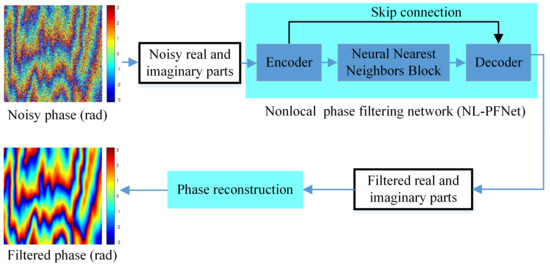
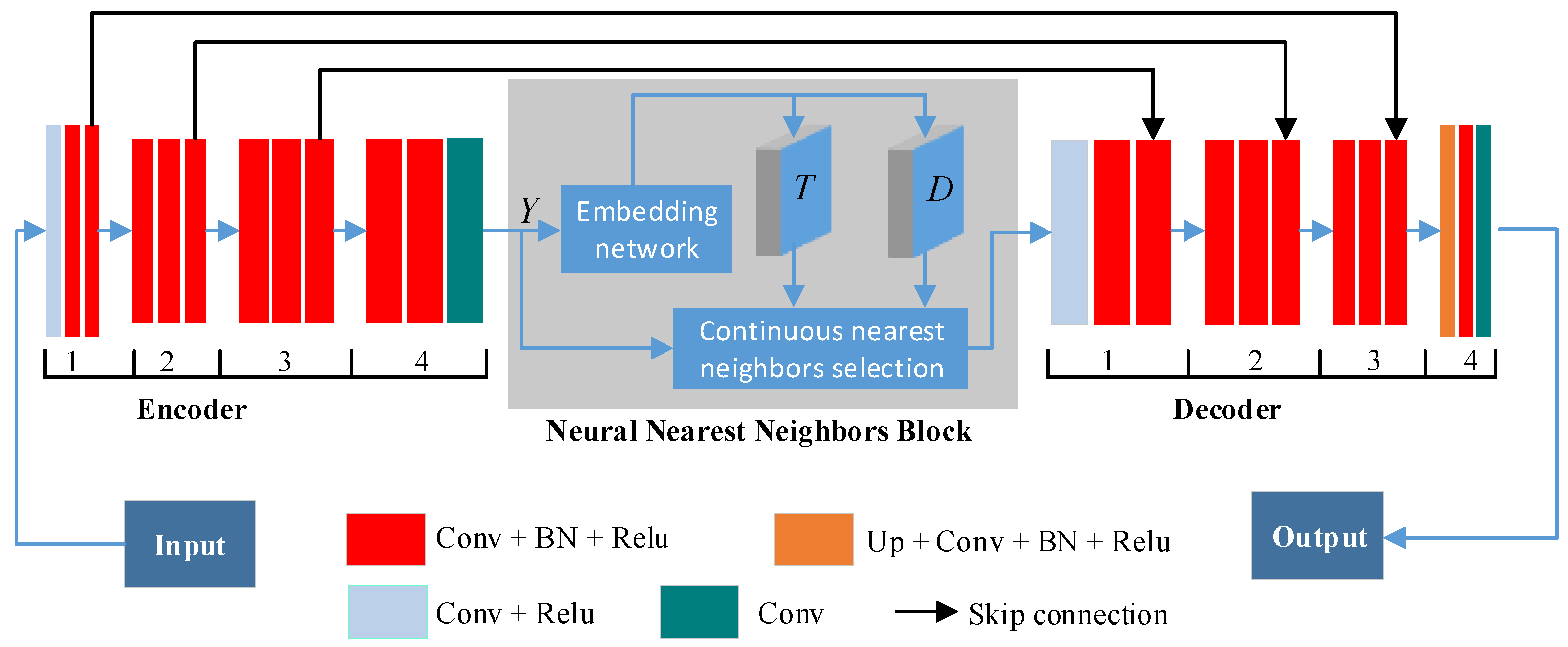
In this paper, we propose a DCNN-based phase-filtering method for InSAR. In this method, a nonlocal phase filtering network (NL-PFNet) is designed based on the encoder–decoder architecture [18] and nonlocal feature selection strategy [19]. Thanks to the powerful phase feature extraction ability of the encoder–decoder structure and the utilization of nonlocal phase information, NL-PFNet can predict accurate filtered phase from a large number of interferometric phase images with different noise levels. Experiments both on simulated and real InSAR data show that the proposed method significantly outperforms the three conventional well-established methods and a deep learning-based method.

The remainder of this paper is organized as follows. In Section 2, we describe the interferometric phase noise model and how to employ neural networks to achieve nonlocal filtering. Section 3 presents the details of the proposed nonlocal phase-filtering method. In Section 4, the filtered results of the proposed method on simulated and real InSAR data are presented. Quantitative and qualitative comparisons with four well-established filtering methods using simulated and real data, and a generalization ability analysis of the proposed method are presented in Section 5. Section 6 gives conclusions and future work.

2. Review and Analysis

In this section, we will review the phase noise model and analyze how to employ neural networks to achieve nonlocal phase filtering.

2.1. Phase Noise Model

The interferometric phase $\varphi$ is obtained by the conjugate multiplication of two co-registered complex SAR images ($S_1$ and $S_2$), which can be expressed as

$$\varphi =\mathrm{angle}(S_1·S_2^{*})$$

(1)

where angle (·) denotes a function that returns the phase angle, and ∗ denotes the complex conjugate. The noise level of the interferometric phase is usually evaluated by the amplitude of the correlation coefficient:

$$\rho =|{\displaystyle \frac{E\{S_1·S_2^{*}\}}{\sqrt{E\left\{\right|S_1{|}^2\}·E\{|S_2{|}^2\}}}}|$$

(2)

where $\rho$ is the coherence. A higher coherence means a lower noise level, and a coherence value of 1 means that the interferometric phase is noise-free (ideal). An additive noise model of the interferometric phase was proven in [7] and can be expressed as

$$\varphi ={\varphi }_c+vs.$$

(3)

where ${\varphi }_c$ is the ideal interferometric phase, and $vs.$ is the zero-mean additive Gaussian noise. ${\varphi }_c$ and $vs.$ are independent variables. The purpose of phase filtering is to estimate ${\varphi }_c$ from $\varphi$.

In the process of interferometric phase filtering, the phase jumps from $-\pi$ to $\pi$ or $\pi$ to $-\pi$ should be preserved in order to correctly unwrap the interferometric phase; therefore, the interferometric phase is usually processed in the complex domain. According to [20], the phase noise model in the complex domain can be expressed as

$$\begin{array}{cc}\hfill & {\varphi }_{real}=cos\left(\varphi \right)=N_{c}cos\left({\varphi }_c\right)+v_r\hfill \\ \hfill & {\varphi }_{imag}=sin\left(\varphi \right)=N_{c}sin\left({\varphi }_c\right)+v_i\hfill \end{array}$$

(4)

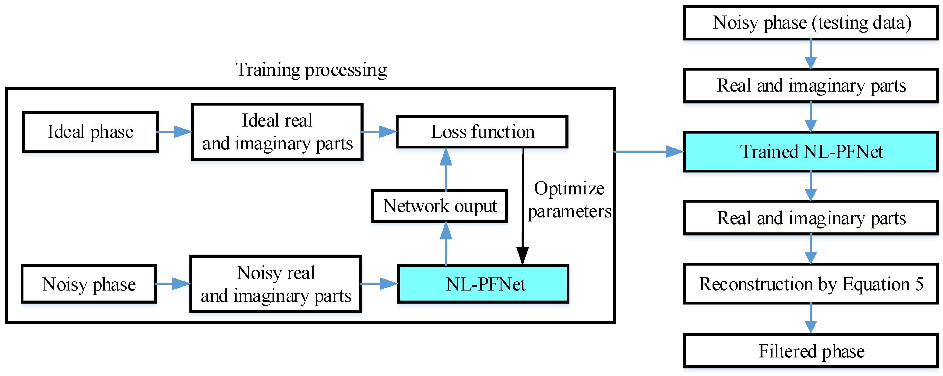
where ${\varphi }_{real}$ and ${\varphi }_{imag}$ are real and imaginary parts of the interferometric phase $\varphi$; $v_r$ and $v_i$ are the zero-mean additive noise; and $N_c$ is a quality index monotonically increasing with the coherence $\rho$. Therefore, the filtering object is converted into the real and imaginary parts rather than the interferometric phase itself. After obtaining the filtered real and imaginary parts, the final filtered interferometric phase can be estimated by

$${\varphi }_c^{\prime }=\mathrm{angle}({\varphi }_{real}^{\prime }+j{\varphi }_{imag}^{\prime }).$$

(5)

2.2. Problem Analysis

According to (5), we can use a neural network to predict the filtered real and imaginary parts of the interferometric phase and then calculate the filtered interferometric phase. Following this processing idea, some methods [16,17] have successfully used DCNNs to achieve phase filtering and rely on the powerful feature extraction capabilities of DCNNs to obtain a filtering performance beyond traditional phase filtering methods to a certain extent, but these methods are achieved based on local neighboring pixels and only use local phase information. However, interferometric phase images have the property of the nonlocal self-similarity, that is, the similar phase fringe structure appears repeatedly in different image regions. If this self-similarity property can be incorporated into network processing to achieve nonlocal phase filtering, it is expected to further improve the accuracy of phase filtering.

In addition, because the noise in the interferometric phase is affected by many factors, such as system thermal noise, time decorrelation, etc., it has strong spatial variability, that is, the noise level is different in different image regions. The spatial variability of the noise requires that the filtering method can handle the interferometric phase images with different noise levels in a balanced manner, otherwise, the low-coherence area may be under-filtered, and the high-coherence area may be over-filtered. Therefore, we use interferometric images with different noise levels as training data to improve the accuracy of the neural network.

3. Proposed Method

Based on the analysis in Section 2, we propose a nonlocal phase filtering method that works via a nonlocal phase filtering network (NL-PFNet) based on the encoder–decoder architecture and nonlocal feature selection strategy. The processing flow of the proposed method is shown in Figure 1. During training, NL-PFNet takes interferometric phase images with different noise levels as inputs and outputs the estimated real and imaginary parts of the interferometric phase. Due to the powerful feature extraction of the encoder–decoder architecture and the use of nonlocal phase information, NL-PFNet can predict the accurate real and imaginary parts of the interferometric phase after training using a large number of interferometric phase images with different noise levels. Finally, the filtered interferometric phase can be obtained by (5). Then, NL-PFNet will be introduced in detail.

Figure 1. The processing flow of the proposed nonlocal phase filtering method.

3.1. Nonlocal Phase Filtering Network

Based on the encoder–decoder structure and nonlocal features’ selection strategy achieved by the neural nearest neighbors block ($N^3$ block), we designed NL-PFNet specialized for interferometric phase filtering. The detailed structure and parameters of NL-PFNet are shown in Figure 2 and Table 1. It can be divided into three sub-networks: encoder part (Encoder), $N^3$ block, and decoder part (Decoder). In the process of building the proposed network, we considered the five following points to adapt to the characteristics of phase filtering. Firstly, the real and imaginary parts of the interferometric phase can be simultaneously fed into the network and the filtered versions can be output at the same time, eliminating the trouble of separate processing. Secondly, the encoder extracts the hierarchical phase features while reducing the image size, which can reduce the computational resource requirements in the $N^3$ block processing. Thirdly, the $N^3$ block is used for the extraction of nonlocal phase feature maps, which is conducive to improving filtering performance. Fourth, the decoder is used to fuse the output of the decoder and $N^3$ block, which allows the nonlocal phase information to be effectively fused in a nonlinear way. Fifth, the skip connections [21] is used for the fusion and complementation of different levels of phase features, which helps to accelerate training while improving filtering accuracy. Then, the encoder–decoder structure and $N^3$ block used in NL-PFNet will be described in detail.

Figure 2. The overall architecture of NL-PFNet. Given the input of the embedding network is Y, the embedding network outputs a pairwise distance matrix D between the query element and nonlocal elements in Y, and a temperature matrix T for each element.

Table 1. Detailed layers and parameters of NL-PFNet.

Block Name	Layer Name	Filter Size	# Channels	Stride	Padding	Output Size
Encoder block-1	Conv + Relu	$3\times 3$	64	1	1	$M\times N\times 64$
	Conv + BN + Relu	$3\times 3$	64	1	1	$M/2\times N/2\times 64$
	Conv + BN + Relu	$3\times 3$	64	2	1	$M/2\times N/2\times 64$
Encoder block-2	Conv + BN + Relu	$3\times 3$	128	1	1	$M/2\times N/2\times 128$
	Conv + BN + Relu	$3\times 3$	128	1	1	$M/2\times N/2\times 128$
	Conv + BN + Relu	$3\times 3$	128	1	1	$M/2\times N/2\times 128$
Encoder block-3	Conv + BN + Relu	$3\times 3$	256	1	1	$M/2\times N/2\times 256$
	Conv + BN + Relu	$3\times 3$	256	1	1	$M/2\times N/2\times 256$
	Conv + BN + Relu	$3\times 3$	256	1	1	$M/2\times N/2\times 256$
Encoder block-4	Conv + BN + Relu	$3\times 3$	256	1	1	$M/2\times N/2\times 256$
	Conv + BN + Relu	$3\times 3$	256	1	1	$M/2\times N/2\times 256$
	Conv	$3\times 3$	8	1	1	$M/2\times N/2\times 8$
	Neural Nearest Neighbors Block					$M/2\times N/2\times 64$
Decoder block-1	Conv + Relu	$3\times 3$	256	1	1	$M/2\times N/2\times 256$
	Conv + BN + Relu	$3\times 3$	256	1	1	$M/2\times N/2\times 256$
	Conv + BN + Relu	$3\times 3$	256	1	1	$M/2\times N/2\times 256$
Decoder block-2	Conv + BN + Relu	$3\times 3$	128	1	1	$M/2\times N/2\times 128$
	Conv + BN + Relu	$3\times 3$	128	1	1	$M/2\times N/2\times 128$
	Conv + BN + Relu	$3\times 3$	128	1	1	$M/2\times N/2\times 128$
Decoder block-3	Conv + BN + Relu	$3\times 3$	64	1	1	$M/2\times N/2\times 64$
	Conv + BN + Relu	$3\times 3$	64	1	1	$M/2\times N/2\times 64$
	Conv + BN + Relu	$3\times 3$	64	1	1	$M/2\times N/2\times 64$
Decoder block-4	Up + Conv + BN + Relu	$3\times 3$	8	1	1	$M\times N\times 8$
	Conv + BN + Relu	$3\times 3$	8	1	1	$M\times N\times 8$
	conv	$3\times 3$	2	1	1	$M\times N\times 2$

3.1.1. Encoder–Decoder Structure

Following the classic encoder–decoder structure [18], the encoder and decoder consist of four encoder blocks and four decoder blocks, and each block consists of three convolution layers. In contrast to [18], the $N^3$ block is utilized to connect the encoder and decoder. To ensure that the $N^3$ block can extract enough phase information in nonlocal processing, the encoder only reduces the image size using the convolution with a stride of two in the encoder block-1; otherwise, the small input feature maps may cause the nonlocal processing to fail. Correspondingly, the decoder only performs the upsampling operation with a scale factor of two in decoder block-4 to ensure that the output image size of the encoder is the same as that of the input image. At the same time, different levels of phase feature maps can be fused by skip connections [21]. In addition, batch normalization (BN) layers are employed to accelerate the network training and boost the network’s performance [22,23].

3.1.2. Neural Nearest Neighbors Block

The nonlocal feature selection strategy is achieved by the $N^3$ block. The block implements nonlocal processing that leverages the property of phase self-similarity and is achieved by a differentiable and continuous version of the k-nearest neighbors (KNN) rule. The $N^3$ block is composed of an embedding network and continuous nearest neighbors selection. Following the classic architecture of the $N^3$ block [19], the embedding network is a multi-layer perceptron with a depth of three and is the same as [19]. Given that the input of the embedding network is Y, the embedding network outputs a pairwise distance matrix D between the query element and nonlocal elements in Y, and a temperature matrix T for each element. The continuous nearest neighbors selection is used to calculate k continuous nearest nonlocal maps and concatenates these maps and Y as output. In the following, how to obtain the k continuous nearest nonlocal maps will be introduced in detail.

The $N^3$ block processes phase images at the patch level, that is, the nonlocal items consist of image patches instead of a single pixel. This can employ the broader contextual phase information. Concretely, given a query image patch q and a dataset of candidate nonlocal self-similarity patches $x_i$ with $i\in I=\{1,\dots ,M\}$, a distance measure function between the query patch and the nonlocal patches can be expressed as

$$d_i=d(q,x_i).$$

(6)

The Euclidean distance is selected as the distance measure function because it works well in the additive noise case [19]. The first element of the weighted vector can be calculated by the softmax function:

$$w_i\left(1\right)=\frac{e^{-d_i/T}}{{\sum }_{i^{\prime }\in I}{e}^{-d_{i^{\prime }}/T}}$$

(7)

Using an iterative scheme to construct the weighted vector including k elements for the KNN rule. The $(j+1)$-th element of the weighted vector can be calculated by

$$w_i(j+1)=\frac{e^{-d_i(j+1)/T}}{{\sum }_{i^{\prime }\in I}{e}^{-d_{i^{\prime }}(j+1)/T}}$$

(8)

where $-d_i(j+1)/T=-d_i\left(j\right)/T+log(1-w_i\left(j\right))$ and $j=1,\dots ,k$. The k continuous nearest neighbors $\left\{X\right(1),\dots ,X(k\left)\right\}$ of the query image patch q can be calculated by

$$X\left(j\right)=\sum _{i\in I}{w}_i\left(j\right)x_i$$

(9)

where the query image patch is obtained by the weighted average of the nonlocal phase information. After processing all image patches, the k continuous nearest nonlocal maps can be obtained.

Following the common parameter configuration of the $N^3$ block [19], the encoder outputs eight feature maps which are fed into the $N^3$ block. For each input feature map of the $N^3$ block, the $N^3$ block computes seven neighbor nonlocal maps, so it outputs 64 feature maps ($8\times 7$ nonlocal maps + 8 input maps). The $N^3$ block calculates seven neighbor nonlocal maps for each input feature map and outputs 64 feature maps. The size of the image patches is set to $10\times 10$ pixels with a stride of five, and 224 nonlocal candidate image patches are matched in an image region with a size of $128\times 128$ pixels for each query image patch.

3.2. Data Generation

To enhance the generalization capability of NL-PFNet, we used a digital elevation model (DEM) to generate interferometric phase images with topography features, which can enhance the phase feature similarity between the simulated and real InSAR data [24,25]. According to the ambiguity height $h_{2\pi }$ of the InSAR system and terrain height, the interferometric phase can be calculated by

$$\varphi (i,j)=\mathrm{angle}(exp(j2\pi \frac{H(i,j)}{h_{2\pi }}))$$

(10)

where $h_{2\pi }$ represents the height change value corresponding to a phase change of $2\pi$. The ambiguity height used to generate samples is set to 92.13 m and is the same as that of the real InSAR data employed in the following experiments. After generating the interferometric phase, its real and imaginary parts can be obtained by (4). In addition, to increase the network’s ability to handle different levels of noise, we generated interferometric phase images with different coherences according to the phase noise model described in Section 2.1, and the coherence range is in $[0.5,0.95]$ with an interval of 0.05. This range can cover most interferometric phase data in practical application [24] and avoid data with coherence $\rho <0.5$ from affecting the filtering performance during the training process.

The DEM used to generate the training data is shown in Figure 3a. These DEM data, which cover the eastern part of Turkey ($2048\times 2048$ pixels), are from SRTM 1Sec HGT. Examples of the ideal and noisy interferometric phase are shown in Figure 3b–d. The topographic features of Figure 3a are similar to those of the real InSAR data employed in the following experiments. To reduce the memory requirement and augment data, the whole interferometric phase image is cut into patches ($256\times 256$ pixels) with 50% overlap. Therefore, the total number of interferometric phase image patches for training is 2250.

Figure 3. Training data: (a) reference DEM; (b) ideal interferometric phase simulated by Figure 3a; (c) noisy interferometric phase with a coherence of 0.75; (d) noisy interferometric phase with a coherence of 0.5.

The DEM data ($1024\times 1024$ pixels) used to generate the testing data are shown in Figure 4a and are different from the one used for training data. The DEM is also from SRTM 1Sec HGT, and the simulation parameter settings are the same as those for the training data. Examples of the ideal and noisy interferometric phase are shown in Figure 4b–d. The total number of interferometric phase image patches for testing is 490; therefore, the ratio of the testing data to the training data is 22%.

Figure 4. Testing data: (a) reference DEM; (b) ideal interferometric phase simulated by Figure 4a; (c) noisy interferometric phase with a coherence of 0.75; and (d) noisy interferometric phase with a coherence of 0.5.

3.3. Loss Function

According to the clean and filtered real and imaginary parts of the interferometric phase, the mean squared error (MSE) is used to optimize the parameters of NL-PFNet. It can be defined as

$$L=\frac{1}{2N}(\parallel {\varphi }_{c,real}-{\varphi }_{real}^{\prime }{\parallel }^2+\parallel {\varphi }_{c,imag}-{\varphi }_{imag}^{\prime }{\parallel }^2)$$

(11)

where N is the number of phase image pixels; ${\varphi }_{c,real}$ and ${\varphi }_{c,imag}$ are the clean real and imaginary parts of the interferometric phase, respectively, and ${\varphi }_{real}^{\prime }$ and ${\varphi }_{imag}^{\prime }$ are the filtered real and imaginary parts of the interferometric phase, respectively.

3.4. Performance Evaluation

In order to evaluate the performance of the proposed method, we conducted a series of experiments using simulated and real InSAR data and compared the proposed method with the Lee filter [7], Goldstein filter [10], InSAR-BM3D filter [14], and a deep learning-based filtering method (PFNet) [17]. Both the qualitative evaluation through visual observation and quantitative evaluation indexes were employed. The quantitative indexes are the number of residues (NOR) [1] remaining after filtering, the MSE between the filtered phase and the corresponding ideal phase, the mean structural similarity index (MSSIM) [26] between the filtered phase and the corresponding ideal phase, and running time (T). Lacking the ideal interferometric phase, the no-reference metric Q [26,27] was used in the experiments on real data. The metric Q can provide a quantitative measure of the phase detail information. A higher Q means that more phase details are preserved after filtering.

All experiments were performed on a computer with an Inter(R) Core(TM) i9-9900k CPU and an NVIDIA GeForce GTX 1080Ti GPU. NL-PFNet was trained using the Adam optimization method [28] with a batch size of two. We trained 50 epochs with an initial learning rate of $1\times {10}^{-3}$ which exponentially decayed from $1\times {10}^{-3}$ to $1\times {10}^{-6}$ on the PyTorch platform, and the training process took approximately 2.5 h.

4. Results

In this section, we used simulated and real InSAR data to verify the effectiveness of the proposed method.

4.1. Experiments on Simulated InSAR Data

We first selected a sample with a coherence of 0.5 to visually analyze the filtering effect of the proposed method and then calculate the mean evaluation indexes of the proposed method for all testing samples.

Figure 5a shows a testing sample with a coherence of 0.5, and its corresponding ideal phase is shown in Figure 5b. Figure 6 shows the filtering result and phase error result obtained by the proposed method. The phase error result was obtained by subtracting the filtered phase from the ideal phase. From Figure 6, we can see that the phase error of the proposed method is close to zero, that is, the filtered phase of the proposed method is close to the ideal phase. In addition, the mean value of NOR, MSSIM, MSE, and T for all testing samples were calculated and listed in Table 2. We can see that the proposed method can filter noise and preserve the phase detail information for simulated InSAR data.

Figure 5. Simulated interferometric phase: (a) clean interferometric phase; (b) noisy version of (a) with a coherence of 0.5.

Figure 6. Filtered result and phase error result of the proposed method on simulated data: (a) filtered interferometric phase; and (b) phase error.

Table 2. Quantitative indexes of the proposed method on simulated data.

Method	NOR	MSSIM	MSE (${\mathbf{Rad}}^2$)	$\mathit{T}$ (s)
No filtering	7217	0.074	3.47	-
Proposed method	0	0.81	0.48	0.023

4.2. Experiments on Real InSAR Data

In this section, a real interferometric phase image ($2048\times 2048$ pixels) covering the eastern part of Turkey was used to evaluate the performance of the proposed method. The interferometric phase (coherence = 0.63) is shown in Figure 7a, and is obtained by the interferometric wide swath mode of the Sentinel-1 SAR satellite. The filtered result obtained by the proposed method is shown in Figure 7b. To better observe the filtering effects, a local area (black rectangle in Figure 7a and the corresponding filtered result are enlarged in Figure 8. For further quantitative analysis, the NOR, the percentage of the reduced residues (PRR), the no-reference metric Q, and running time were calculated and listed in Table 3. We can see that the proposed method can filter noise and preserve the phase detail information for real InSAR data.

Figure 7. Real InSAR data and the filtered result using the proposed methods: (a) a real interferometric phase image of Sentinel-1; (b) filtered result.

Figure 8. Filtered results of a local area in Figure 7a (black rectangle) using the proposed method: (a) black rectangle area in Figure 7a; and (b) filtered result.

Table 3. Quantitative indexes of the proposed method on real InSAR data.

Method	NOR	PRR (%)	Metric Q	$\mathit{T}\left(\mathit{s}\right)$
No filtering	546,647	0	2.08	-
Proposed method	1624	99.70	31.70	5.35

5. Discussion

In this section, we use simulated and real InSAR data to compare the proposed method with the Lee filter, Goldstein filter, InSAR-BM3D filter and PFNet.

5.1. Comparison Experiments on Simulated InSAR Data

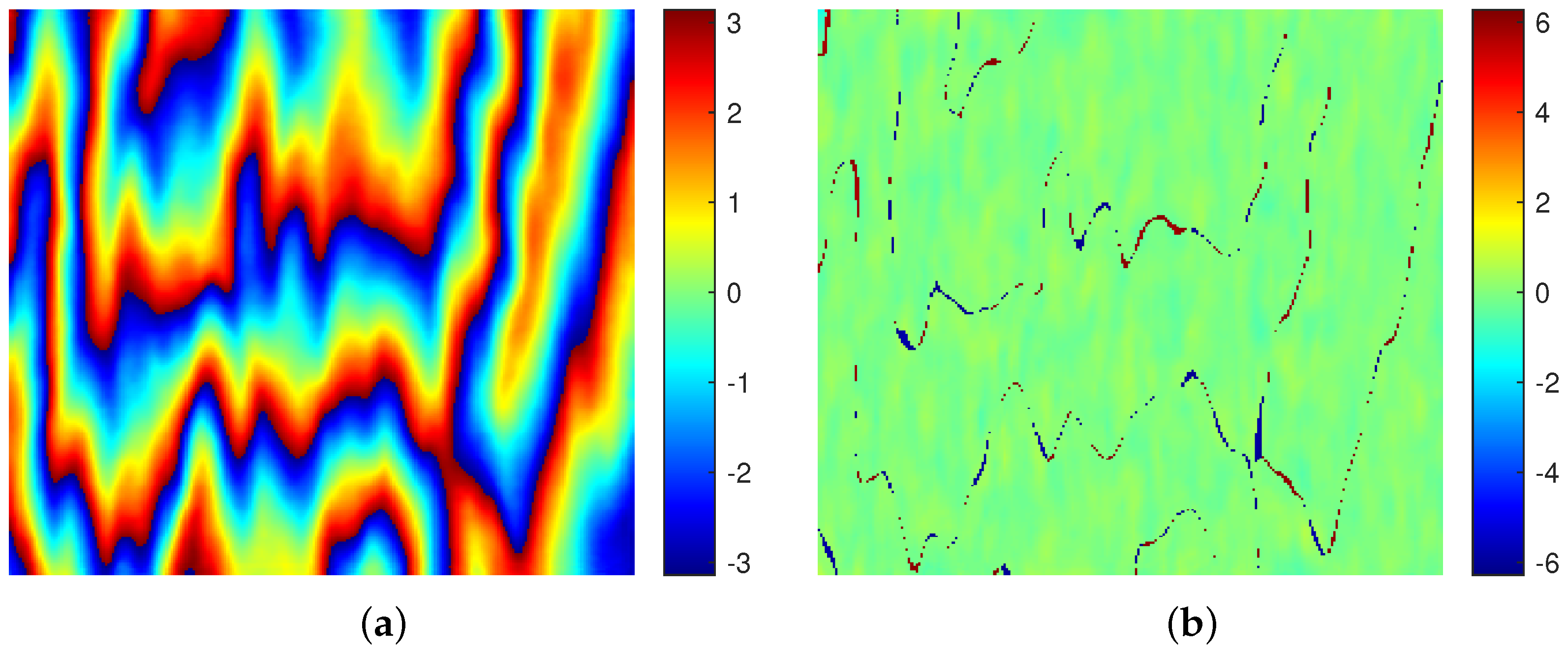
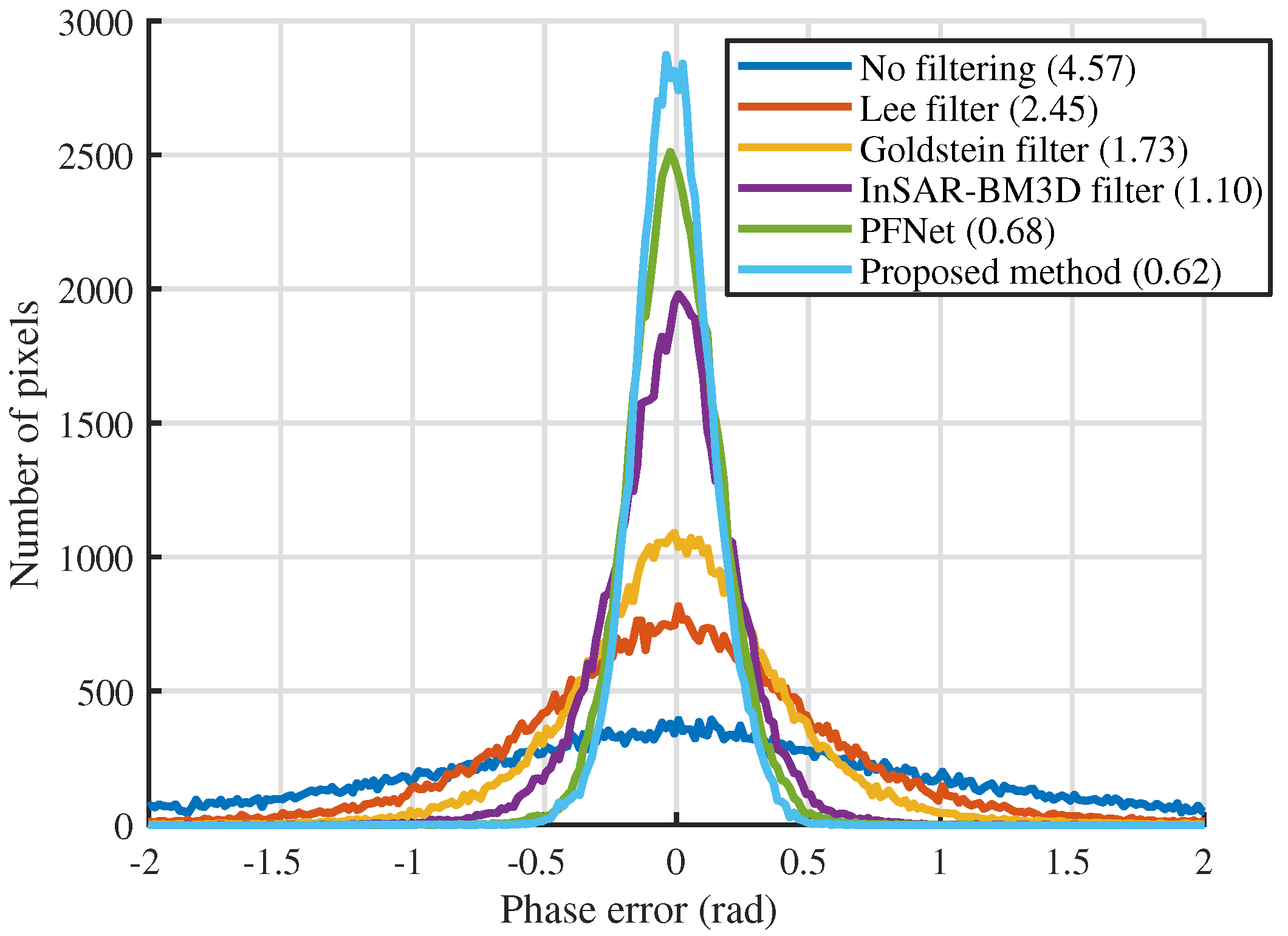
Figure 9 shows the filtering results of Figure 5a and phase error results obtained by the four reference methods. From Figure 6 and Figure 9, we can see that the phase error of the proposed method is closer to zero than other methods, that is, the filtered phase of the proposed method is closest to the ideal phase. In order to further verify this inference, the fitted histogram curves of the phase errors are given in Figure 10. The fitted histogram curve can clearly compare the error distribution of various methods. As can be seen from Figure 10, the error curve of the proposed method is sharper near zero than other methods, that is, the proposed method outperforms other methods from the perspective of phase error.

Figure 9. Filtered results (top) and phase error results (bottom) of the four reference methods on simulated data: (a) Lee filter; (b) Goldstein filter; (c) InSAR-BM3D filter; and (d) PFNet.

Figure 10. Fitted phase error histogram curves of the five methods. The standard deviation of the six curves are 4.57, 2.45, 1.73, 1.10, 0.68 and 0.62.

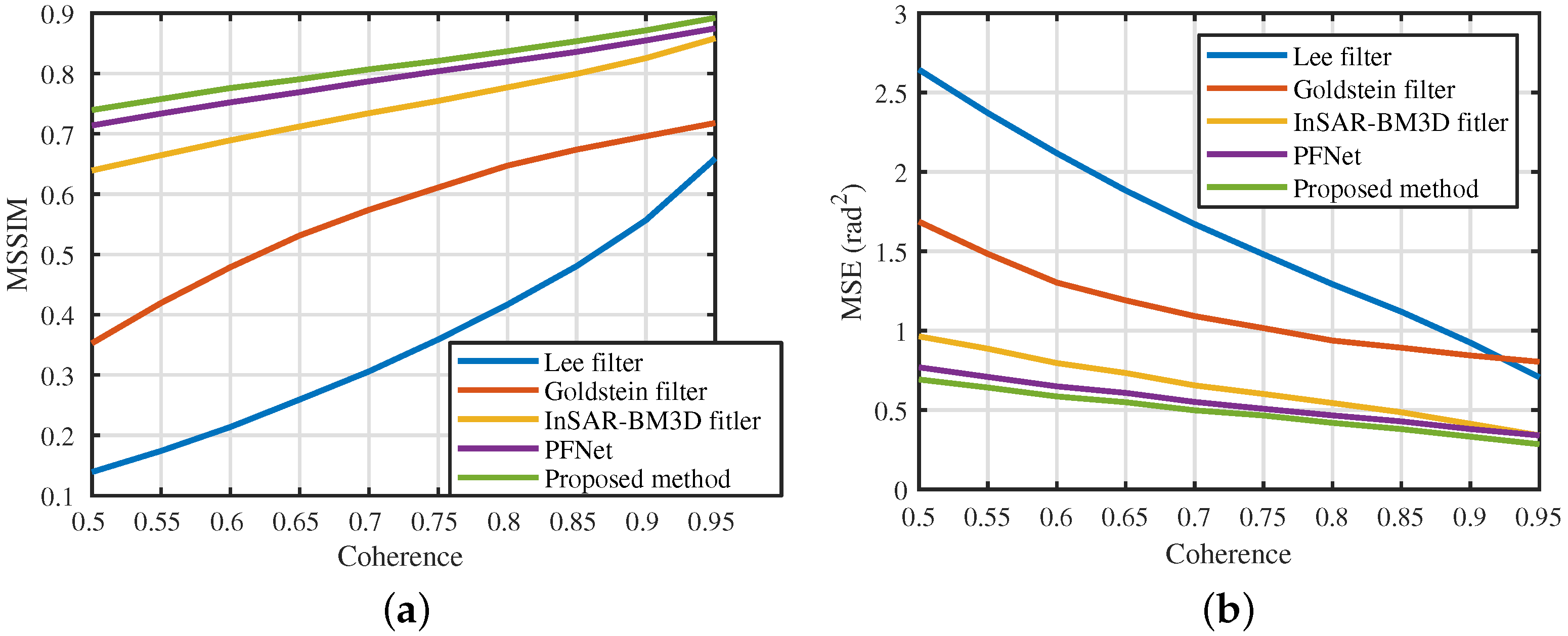
To verify the performance of the proposed method under different noise levels, the quantitative indexes were calculated for all testing samples with the same coherences, and the results are shown in Figure 11. From Figure 11, we can see that the proposed method has the highest MSSIM and lowest MSE among the five methods under all considered cases, that is, the proposed method can obtain the highest filtering performance. In addition, the mean NOR, MSSIM, MSE, and T of the four reference methods for all testing samples were calculated and listed in Table 4. From Table 2 and Table 4, we can see that the InSAR-BM3D filter, PFNet, and the proposed method have sufficient filtering power to filter out all residues from the perspective of NOR. Among these five methods, the proposed method has the highest MSSIM and the smallest MSE. Compared with the InSAR-BM3D filter and PFNet, the MSSIM of the proposed method is 8% and 3% higher, respectively, and the MSE of the proposed method is 25% and 11% higher, respectively. This indicates that the proposed method has the best filtering performance. In addition, the proposed method has a significant advantage of computational efficiency compared to traditional methods. Compared with PFNet, the proposed method has the same level of running time because the required running time for nonlocal processing is also small when the image size is small.

Figure 11. Quantitative indexes of the proposed and reference methods for phase filtering results on simulated images with different coherences: (a) mean structural similarity index (MSSIM); (b) mean square error (MSE).

Table 4. Quantitative indexes of the reference methods on simulated images.

Method	NOR	MSSIM	MSE (${\mathbf{Rad}}^2$)	$\mathit{T}$ (s)
Lee filter	268	0.36	1.62	2.88
Goldstein filter	14	0.57	1.12	2.70
InSAR-BM3D filter	0	0.75	0.64	6.95
PFNet	0	0.79	0.54	0.028

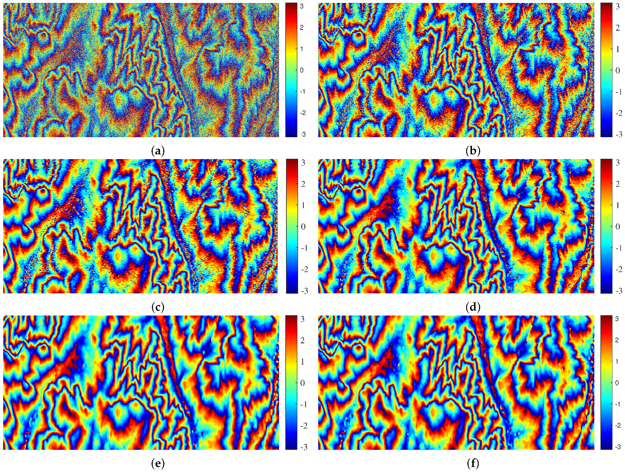
5.2. Comparison Experiments on Real InSAR Data

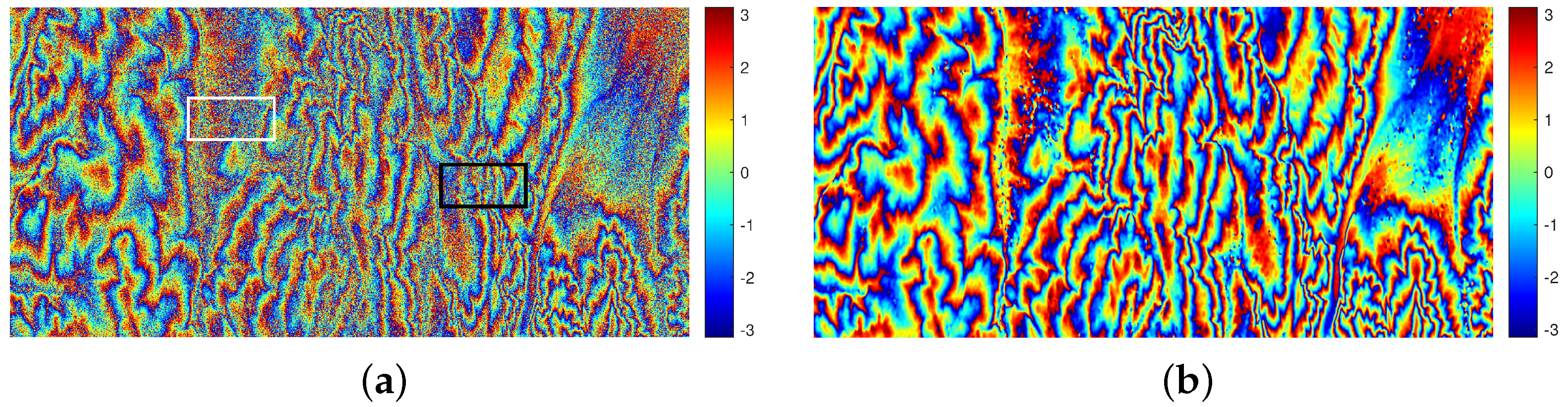
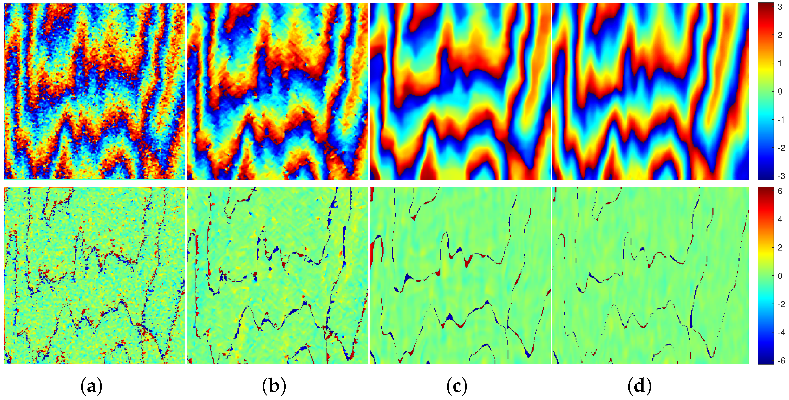
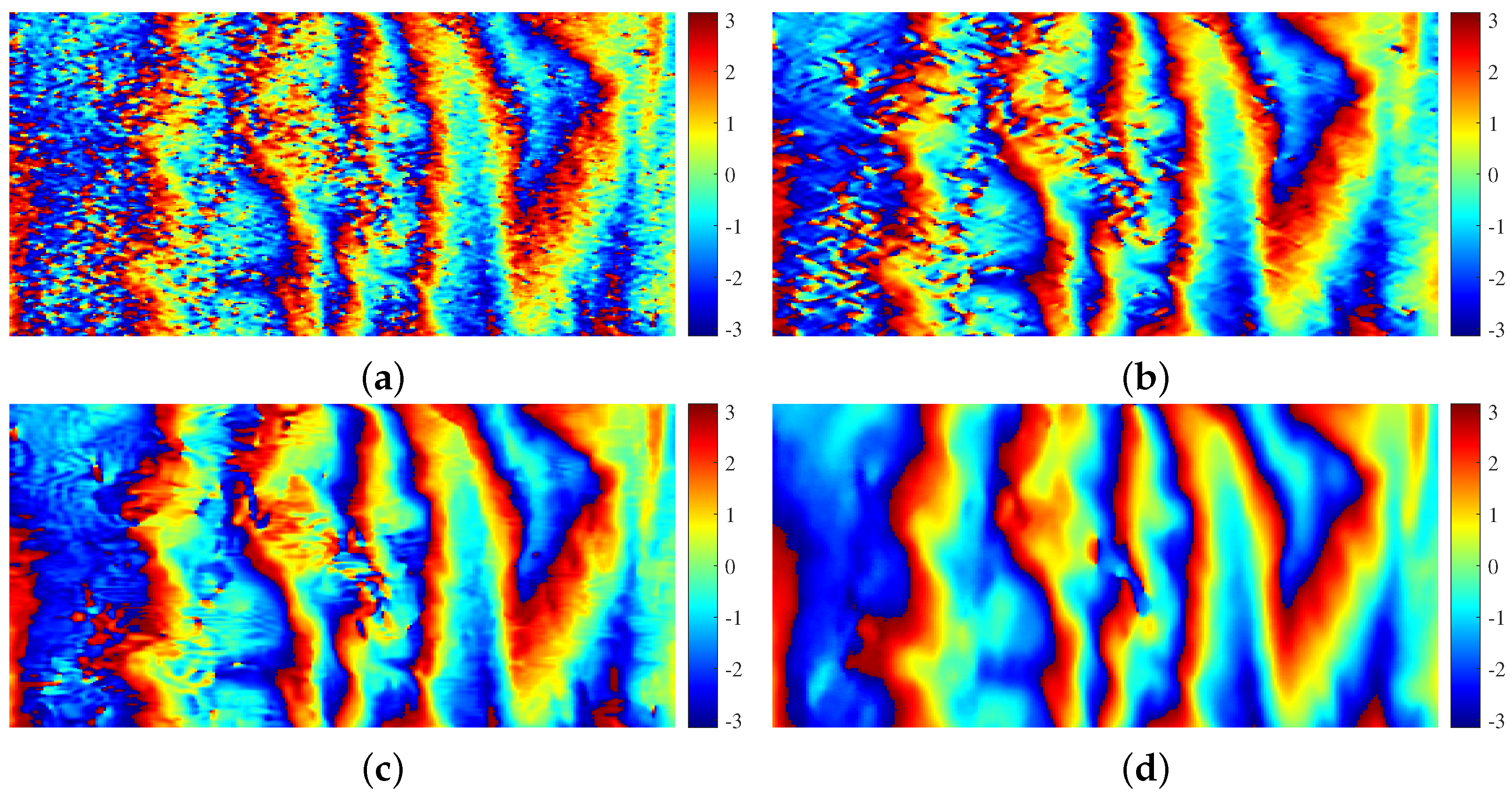
The filtered results of Figure 7a obtained by the four reference methods are shown in Figure 12a–d, respectively. To better observe the filtering effects, a local area (black rectangle in Figure 7a) and the corresponding filtered results are enlarged in Figure 13. From Figure 7, Figure 8, Figure 12 and Figure 13, we can see that compared with PFNet and the proposed method, the denoising power of the Lee filter, Goldstein filter and InSAR-BM3D filter is not enough. Compared with the proposed method, the result of PFNet is over-filtered, that is, more phase detail information is lost. However, the proposed method better balances denoising and phase detail preservation.

Figure 12. Filtered results of Figure 7a using the four reference methods: (a) Lee filter; (b) Goldstein filter; (c) InSAR-BM3D filter; and (d) PFNet.

Figure 13. Filtered results of a local area in Figure 7a (black rectangle) using the four reference methods: (a) Lee filter; (b) Goldstein filter; (c) InSAR-BM3D filter; and (d) PFNet.

For further quantitative analysis, the evaluation indexes of the four reference methods were calculated and listed in Table 5. From Table 3 and Table 5, it can be seen that compared with the Lee filter, Goldstein filter and InSAR-BM3D filter, the PRR and metric Q of the proposed method and PFNet are significantly higher, which indicates that the proposed method and PFNet have better filtering performance. Comparing the proposed method and PFNet, although the proposed method has a lower PRR, it has a higher metric Q. This indicates that PFNet loses more phase detail information due to the excessive denoising ability, while the proposed method maintains the balance of denoising and phase detail preservation. Compared with the InSAR-BM3D filter and PFNet, the metric Q of the proposed method is 25% and 9% higher, respectively. Furthermore, due to the time consumption of nonlocal phase information processing, the running time of the proposed method is higher than PFNet, but still several tens of times less than the Lee filter, Goldstein filter, and InSAR-BM3D filter.

Table 5. Quantitative indexes of the four reference methods on real InSAR data.

Method	NOR	PRR (%)	Metric Q	$\mathit{T}\left(\mathit{s}\right)$
Lee Filter	85,930	84.28	9.93	180.26
Goldstein Filter	31,024	94.32	17.55	174.73
InSAR-BM3D Filter	5936	98.91	25.44	483.47
PFNet	415	99.92	29.02	0.25

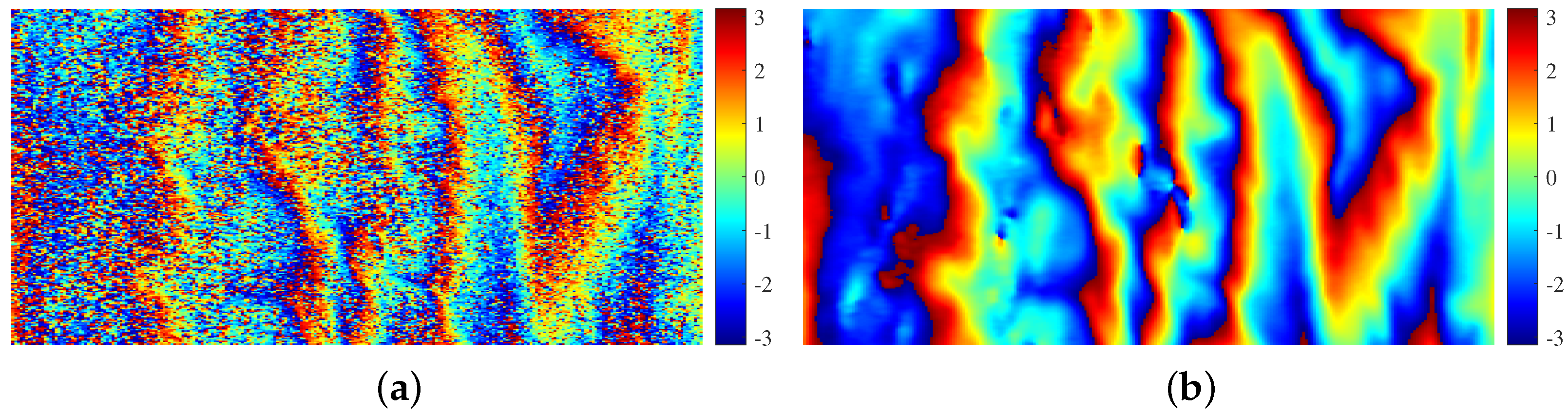
5.3. Generalization Ability to Real InSAR Data

To further analyze the filtering performance of the proposed method for low-coherence areas, a low-coherence region (coherence = 0.44) of Figure 7a (white rectangle) and the corresponding filtered results obtained by the proposed and reference methods are shown in Figure 14. For further quantitative analysis, the evaluation indexes of the five methods were calculated and listed in Table 6. Comparing the proposed method and PFNet, although the proposed method has a lower PRR, it has a higher metric Q. Compared with the InSAR-BM3D filter and PFNet, the metric Q of the proposed method is 37% and 19% higher, respectively. Therefore, we can see that the proposed method maintains the balance of denoising and phase detail preservation for the low-coherence area better than the reference methods.

Figure 14. Filtered results of a low-coherence area using the proposed and reference methods: (a) a low-coherence area (the white rectangle in Figure 7a); (b) Lee filter; (c) Goldstein filter; (d) InSAR-BM3D filter; (e) PFNet; and (f) proposed method.

Table 6. Quantitative indexes of the proposed and reference methods on a low-coherence area of real InSAR data (the white rectangle in Figure 7a).

Method	NOR	PRR (%)	Metric Q
No filtering	11,142	0	1.80
Lee filter	3011	72.98	11.17
Goldstein filter	1550	86.09	17.16
InSAR-BM3D filter	585	94.75	27.10
PFNet	59	99.47	32.13
Proposed method	78	99.30	37.71

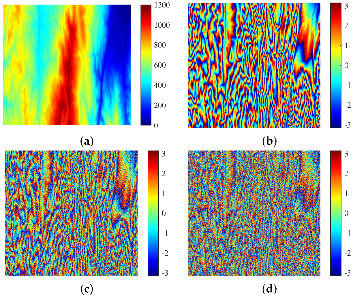
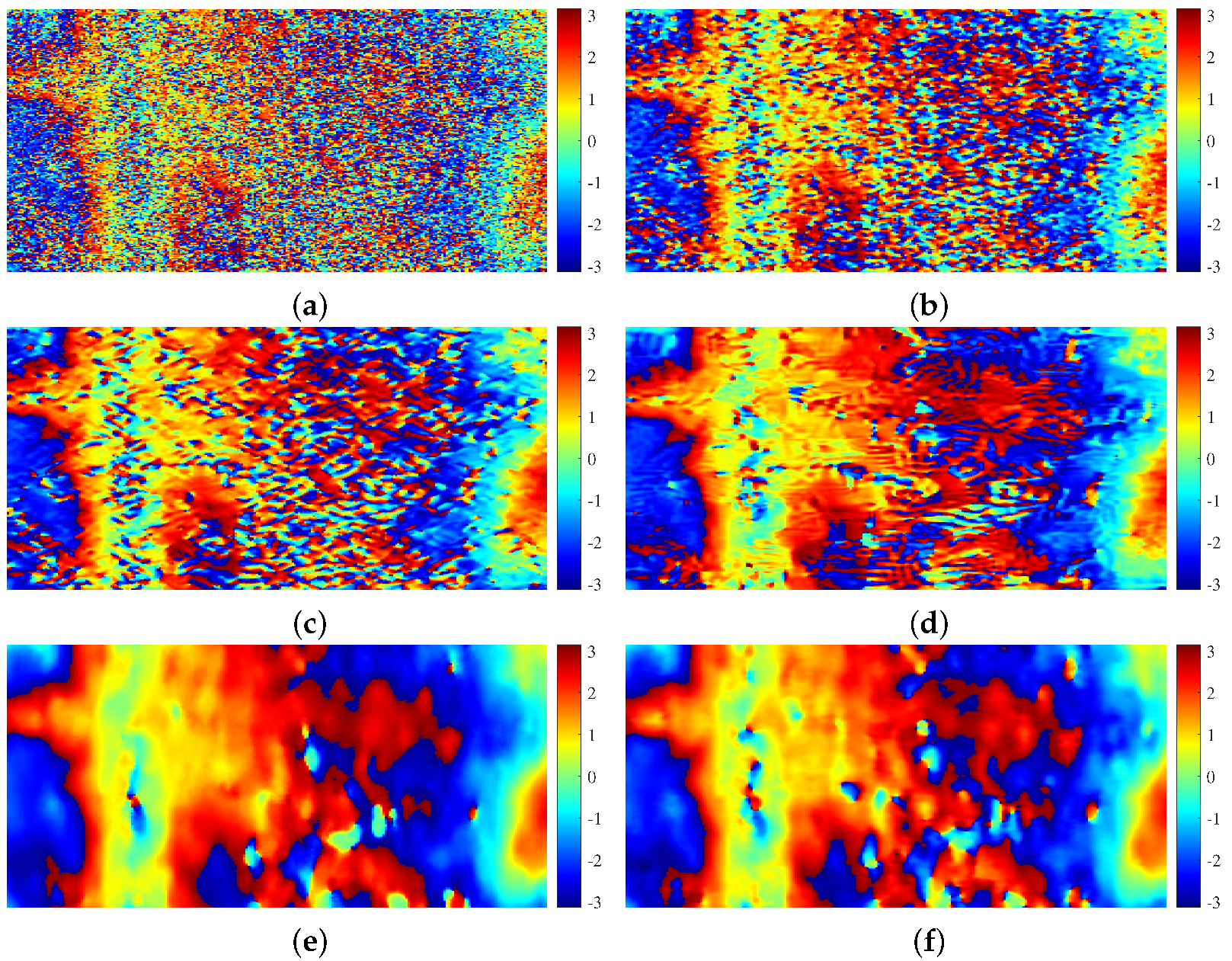
To verify the generalization ability of the proposed method for different studied areas, we processed the real InSAR data with different terrain from the training data. The real interferometric phase image also comes from the interferometric wide swath mode of the Sentinel-1 SAR satellite. The interferometric phase ($1024\times 1024$ pixels, coherence = 0.62) is shown in Figure 15a. The filtered results obtained by the proposed and reference methods are shown in Figure 15b–f, respectively. For further quantitative analysis, the evaluation indexes of the five methods were calculated and listed in Table 7. From Figure 15 and Table 7, we can see that the proposed method maintains the balance of denoising and phase detail preservation better than the reference methods. Compared with the InSAR-BM3D filter, the metric Q of the proposed method is 24% higher. According to Section 5.2, in the case of the real data with the same terrain as the training data, the improvement of the metric Q is 25% higher. It can be seen that there is a slight drop in filtering performance when the terrain of the study area is different from that of the training data. Therefore, to a certain extent, the proposed method has good generalization ability to different studied areas in this experiment. In practical applications, the need to regenerate training data and retrain can be determined based on a combination of the three following factors: the required filtering performance, the required training time and whether there is the DEM of the studied area to generate training data. Furthermore, the ambiguity height of the InSAR system directly affects the density of phase fringes related to the filtering performance. Therefore, to enhance the phase feature similarity between simulated and real InSAR data [24,25], the ambiguity height used in the process of generating the training data is the same as that of the real InSAR system.

Figure 15. Filtered results of Figure 15a using the reference and proposed methods: (a) a real interferometric phase image of Sentinel-1 with a different terrain from the training data; (b) Lee filter; (c) Goldstein filter; (d) InSAR-BM3D filter; (e) PFNet; and (f) proposed method.

Table 7. Quantitative indexes of the proposed and reference methods on real InSAR data with different terrain from the training data.

Method	NOR	PRR (%)	Metric Q	$\mathit{T}\left(\mathit{s}\right)$
No filtering	139,099	0	1.99	-
Lee filter	19,805	85.76	10.74	44.82
Goldstein filter	6288	95.48	19.11	44.44
InSAR-BM3D filter	893	99.36	27.65	120.11
PFNet	94	99.93	32.20	0.14
Proposed method	113	99.92	34.17	1.37

In addition, as with the terrain-induced interferometric phase, the deformation-induced interferometric phase, such as the co-seismic interferogram, also has the property of the nonlocal phase self-similarity. Therefore, the proposed nonlocal filtering method should also be applicable to deformation-induced interferometric phase filtering and can obtain a better filtering performance than the four reference methods used in this paper.

6. Conclusions

In this paper, a nonlocal InSAR phase filtering method via NL-PFNet was proposed to improve the filtering performance. NL-PFNet is designed based on the encoder–decoder structure and nonlocal feature selection strategy. Thanks to the powerful phase feature extraction ability of the encoder–decoder structure and the utilization of nonlocal information in the $N^3$ block, NL-PFNet can predict an accurate filtered phase after training using a large number of interferometric phase images with different noise levels. Experiments both on simulated and real InSAR data show that the proposed method significantly outperforms the three traditional well-established methods and another deep learning-based method. In experiments on simulated data, compared with the InSAR-BM3D filter and PFNet, the MSE of the proposed method is 25% and 11% lower, respectively. Furthermore, when processing the Sentinel-1 interferometric phase, compared with the InSAR-BM3D filter and PFNet, the metric Q of the proposed method is 25% and 9% higher, respectively. In addition, the running time of the proposed method is tens of times less than that of the traditional filtering methods. In future work, to further improve filtering performance, we will combine more advanced nonlocal processing methods with the deep learning networks to achieve InSAR phase filtering.

References

- Bamler, R.; Hartl, P. Synthetic aperture radar interferometry. Inverse Probl. 1998, 14, R1. [Google Scholar] [CrossRef]
- Zhu, X.; Wang, Y.; Montazeri, S.; Ge, N. A Review of Ten-Year Advances of Multi-Baseline SAR Interferometry Using TerraSAR-X Data. Remote Sens. 2018, 10, 1374. [Google Scholar] [CrossRef] [Green Version]
- Richter, N.; Froger, J.L. The role of Interferometric Synthetic Aperture Radar in detecting, mapping, monitoring, and modelling the volcanic activity of Piton de la Fournaise, La Réunion: A review. Remote Sens. 2020, 12, 1019. [Google Scholar] [CrossRef] [Green Version]
- Huang, L.; Hajnsek, I. Polarimetric Behavior for the Derivation of Sea Ice Topographic Height from TanDEM-X Interferometric SAR Data. IEEE J. Sel. Top. Appl. Earth Obs. Remote Sens. 2020, 14, 1095–1110. [Google Scholar] [CrossRef]
- Wang, H.; Fu, H.; Zhu, J.; Liu, Z.; Zhang, B.; Wang, C.; Li, Z.; Hu, J.; Yu, Y. Estimation of subcanopy topography based on single-baseline TanDEM-X InSAR data. J. Geod. 2021, 95, 1–19. [Google Scholar] [CrossRef]
- Xu, G.; Gao, Y.; Li, J.; Xing, M. InSAR phase denoising: A review of current technologies and future directions. IEEE Geosci. Remote Sens. Mag. 2020, 8, 64–82. [Google Scholar] [CrossRef] [Green Version]
- Lee, J.S.; Papathanassiou, K.P.; Ainsworth, T.L.; Grunes, M.R.; Reigber, A. A new technique for noise filtering of SAR interferometric phase images. IEEE Trans. Geosci. Remote Sens. 1998, 36, 1456–1465. [Google Scholar]
- Vasile, G.; Trouvé, E.; Lee, J.S.; Buzuloiu, V. Intensity-driven adaptive-neighborhood technique for polarimetric and interferometric SAR parameters estimation. IEEE Trans. Geosci. Remote Sens. 2006, 44, 1609–1621. [Google Scholar] [CrossRef] [Green Version]
- Li, T.; Chen, K.S.; Lee, J.S. Enhanced Interferometric Phase Noise Filtering of the Refined InSAR Filter. IEEE Geosci. Remote Sens. Lett. 2019, 17, 1528–1532. [Google Scholar] [CrossRef]
- Goldstein, R.M.; Werner, C.L. Radar interferogram filtering for geophysical applications. Geophys. Res. Lett. 1998, 25, 4035–4038. [Google Scholar] [CrossRef] [Green Version]
- Song, R.; Guo, H.; Liu, G.; Perski, Z.; Fan, J. Improved Goldstein SAR interferogram filter based on empirical mode decomposition. IEEE Geosci. Remote Sens. Lett. 2013, 11, 399–403. [Google Scholar] [CrossRef]
- Chi, B.; Zhuang, H.; Fan, H.; Yu, Y.; Peng, L. An adaptive patch-based goldstein filter for interferometric phase denoising. Int. J. Remote Sens. 2021, 42, 6746–6761. [Google Scholar] [CrossRef]
- Deledalle, C.A.; Denis, L.; Tupin, F. NL-InSAR: Nonlocal interferogram estimation. IEEE Trans. Geosci. Remote Sens. 2010, 49, 1441–1452. [Google Scholar] [CrossRef]
- Sica, F.; Cozzolino, D.; Zhu, X.X.; Verdoliva, L.; Poggi, G. INSAR-BM3D: A nonlocal filter for SAR interferometric phase restoration. IEEE Trans. Geosci. Remote Sens. 2018, 56, 3456–3467. [Google Scholar] [CrossRef] [Green Version]
- Xu, H.; Li, Z.; Li, S.; Liu, W.; Li, J.; Liu, A.; Li, W. A Nonlocal Noise Reduction Method Based on Fringe Frequency Compensation for SAR Interferogram. IEEE J. Sel. Top. Appl. Earth Obs. Remote Sens. 2021, 14, 9756–9767. [Google Scholar] [CrossRef]
- Sun, X.; Zimmer, A.; Mukherjee, S.; Kottayil, N.K.; Ghuman, P.; Cheng, I. DeepInSAR—A Deep Learning Framework for SAR Interferometric Phase Restoration and Coherence Estimation. Remote Sens. 2020, 12, 2340. [Google Scholar] [CrossRef]
- Pu, L.; Zhang, X.; Zhou, Z.; Shi, J.; Wei, S.; Zhou, Y. A Phase Filtering Method with Scale Recurrent Networks for InSAR. Remote Sens. 2020, 12, 3453. [Google Scholar] [CrossRef]
- Ronneberger, O.; Fischer, P.; Brox, T. U-net: Convolutional networks for biomedical image segmentation. In Proceedings of the International Conference on Medical Image Computing and Computer-Assisted Intervention, Munich, Germany, 5–9 October 2015; Springer: Berlin/Heidelberg, Germany, 2015; pp. 234–241. [Google Scholar]
- Plötz, T.; Roth, S. Neural Nearest Neighbors Networks. Adv. Neural Inf. Process. Syst. 2018, 31, 1087–1098. [Google Scholar]
- Lopez-Martinez, C.; Fabregas, X. Modeling and reduction of SAR interferometric phase noise in the wavelet domain. IEEE Trans. Geosci. Remote Sens. 2002, 40, 2553–2566. [Google Scholar] [CrossRef] [Green Version]
- Mao, X.; Shen, C.; Yang, Y.B. Image restoration using very deep convolutional encoder-decoder networks with symmetric skip connections. Adv. Neural Inf. Process. Syst. 2016, 29, 2802–2810. [Google Scholar]
- Ioffe, S.; Szegedy, C. Batch normalization: Accelerating deep network training by reducing internal covariate shift. In Proceedings of the International Conference on Machine Learning, Lille, France, 6–11 July 2015; pp. 448–456. [Google Scholar]
- Zhang, K.; Zuo, W.; Chen, Y.; Meng, D.; Zhang, L. Beyond a gaussian denoiser: Residual learning of deep cnn for image denoising. IEEE Trans. Image Process. 2017, 26, 3142–3155. [Google Scholar] [CrossRef] [PubMed] [Green Version]
- Pu, L.; Zhang, X.; Zhou, Z.; Li, L.; Zhou, L.; Shi, J.; Wei, S. A Robust InSAR Phase Unwrapping Method via Phase Gradient Estimation Network. Remote Sens. 2021, 13, 4564. [Google Scholar] [CrossRef]
- Zhou, L.; Yu, H.; Lan, Y. Deep Convolutional Neural Network-Based Robust Phase Gradient Estimation for Two-Dimensional Phase Unwrapping Using SAR Interferograms. IEEE Trans. Geosci. Remote Sens. 2020, 58, 4653–4665. [Google Scholar] [CrossRef]
- Zhu, X.; Milanfar, P. Automatic Parameter Selection for Denoising Algorithms Using a No-Reference Measure of Image Content. IEEE Trans. Image Process. 2010, 19, 3116–3132. [Google Scholar]
- Fang, D.; Lv, X.; Wang, Y.; Lin, X.; Qian, J. A Sparsity-Based InSAR Phase Denoising Algorithm Using Nonlocal Wavelet Shrinkage. Remote Sens. 2016, 8, 830. [Google Scholar] [CrossRef] [Green Version]
- Kingma, D.P.; Ba, J. Adam: A method for stochastic optimization. arXiv 2014, arXiv:1412.6980. [Google Scholar]
Publisher’s Note: MDPI stays neutral with regard to jurisdictional claims in published maps and institutional affiliations. |
© 2022 by the authors. Licensee MDPI, Basel, Switzerland. This article is an open access article distributed under the terms and conditions of the Creative Commons Attribution (CC BY) license (https://creativecommons.org/licenses/by/4.0/).