
Development of Semantic Maps of Vegetation Cover from UAV Images to Support Planning and Management in Fine-Grained Fire-Prone Landscapes


Abstract
:1. Introduction
1.1. Remote Sensing and Land Cover Mapping
1.2. Case Study: Fire Prone Mediterranean Landscapes
1.3. Objectives
2. Materials and Methods
2.1. Study Area
2.2. Data Description
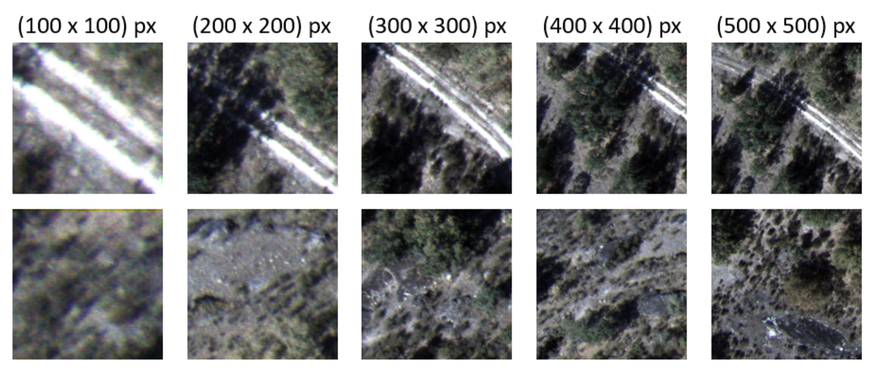
- One (800 × 800) px tile derived from the same image from which training tiles were taken, which was not previously used for training;
- Two (800 × 800) px tiles derived from two other images that were taken during the same flight;
- Two (800 × 800) px tiles derived from one image that was taken during the same season but in a following year (August 2020—summer season);
- Two (800 × 800) px tiles derived from one image that was taken during a different season (December 2019—winter season).
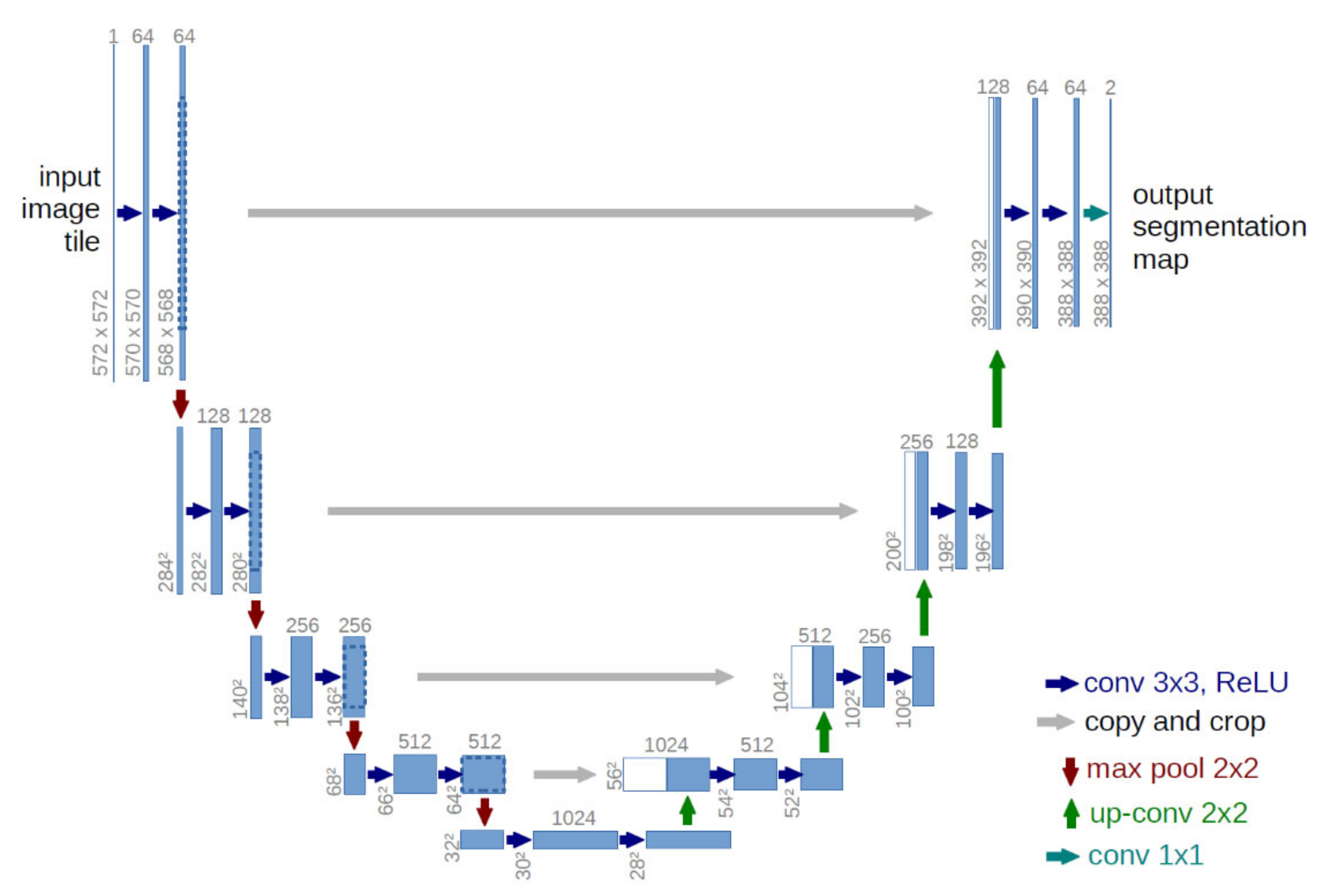
2.3. Model
2.4. Model Training
2.5. Evaluation Method
3. Results
3.1. Preliminary Analysis in the Training Sets
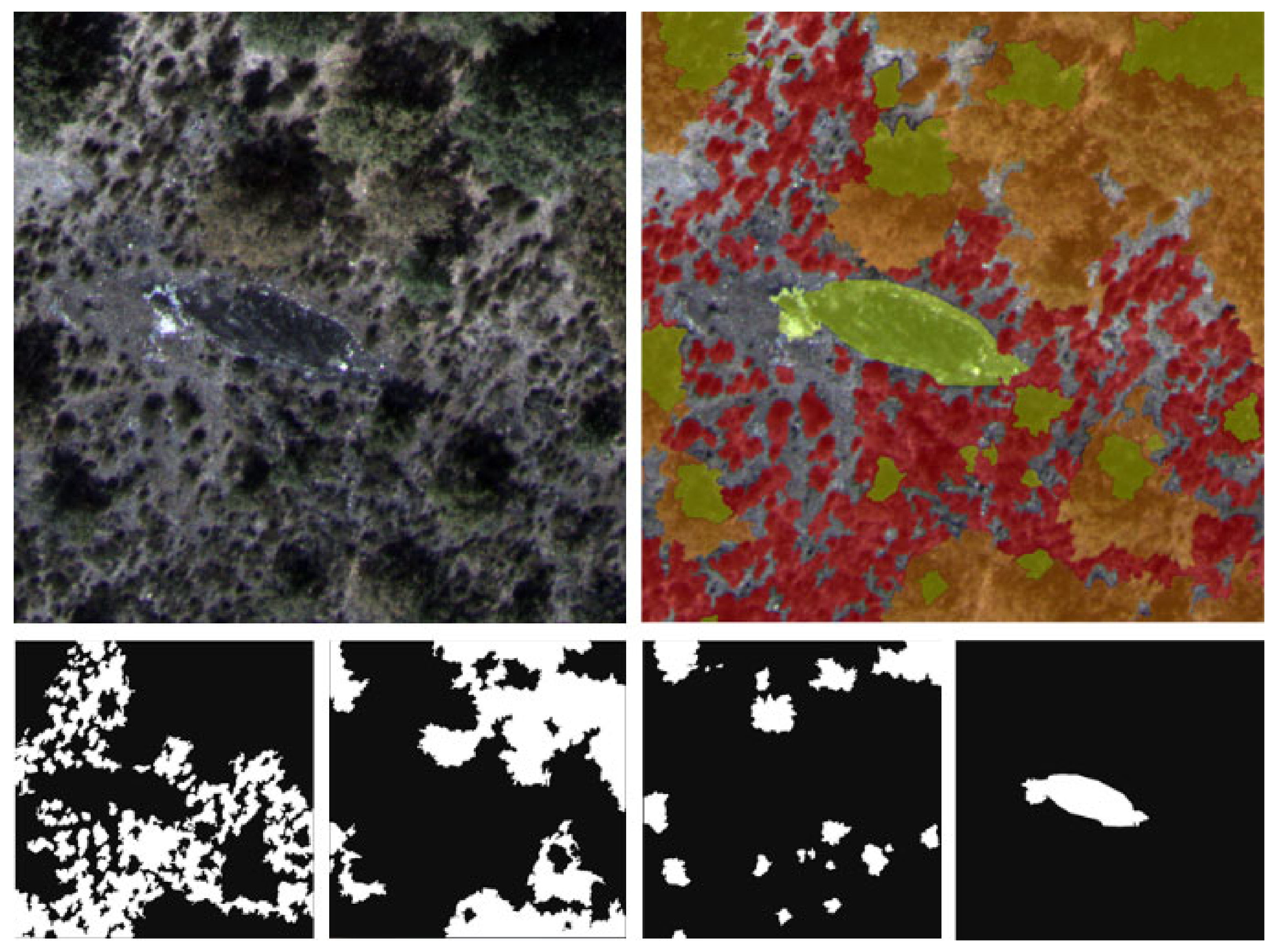
3.1.1. Multi-Class Segmentation
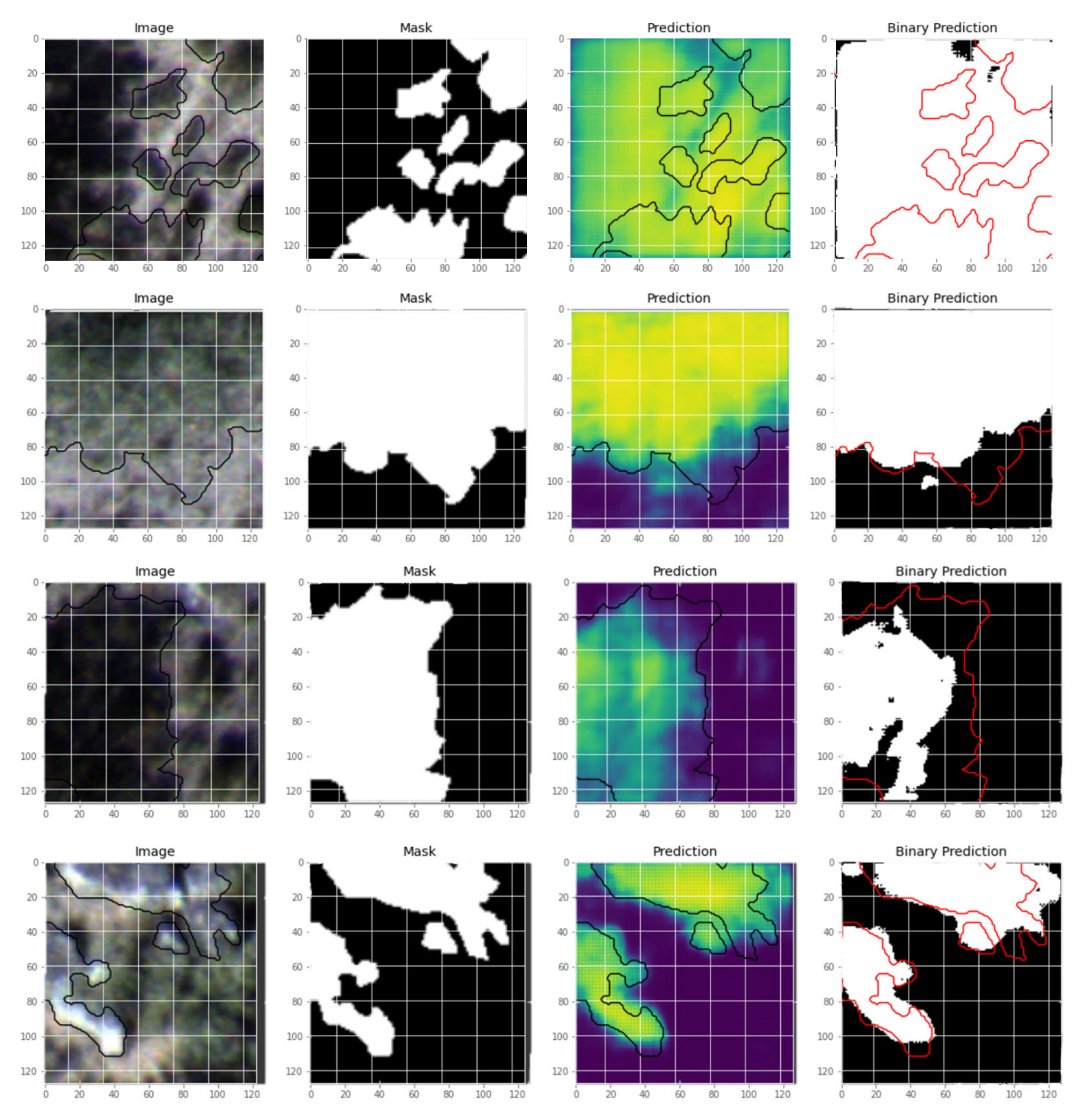
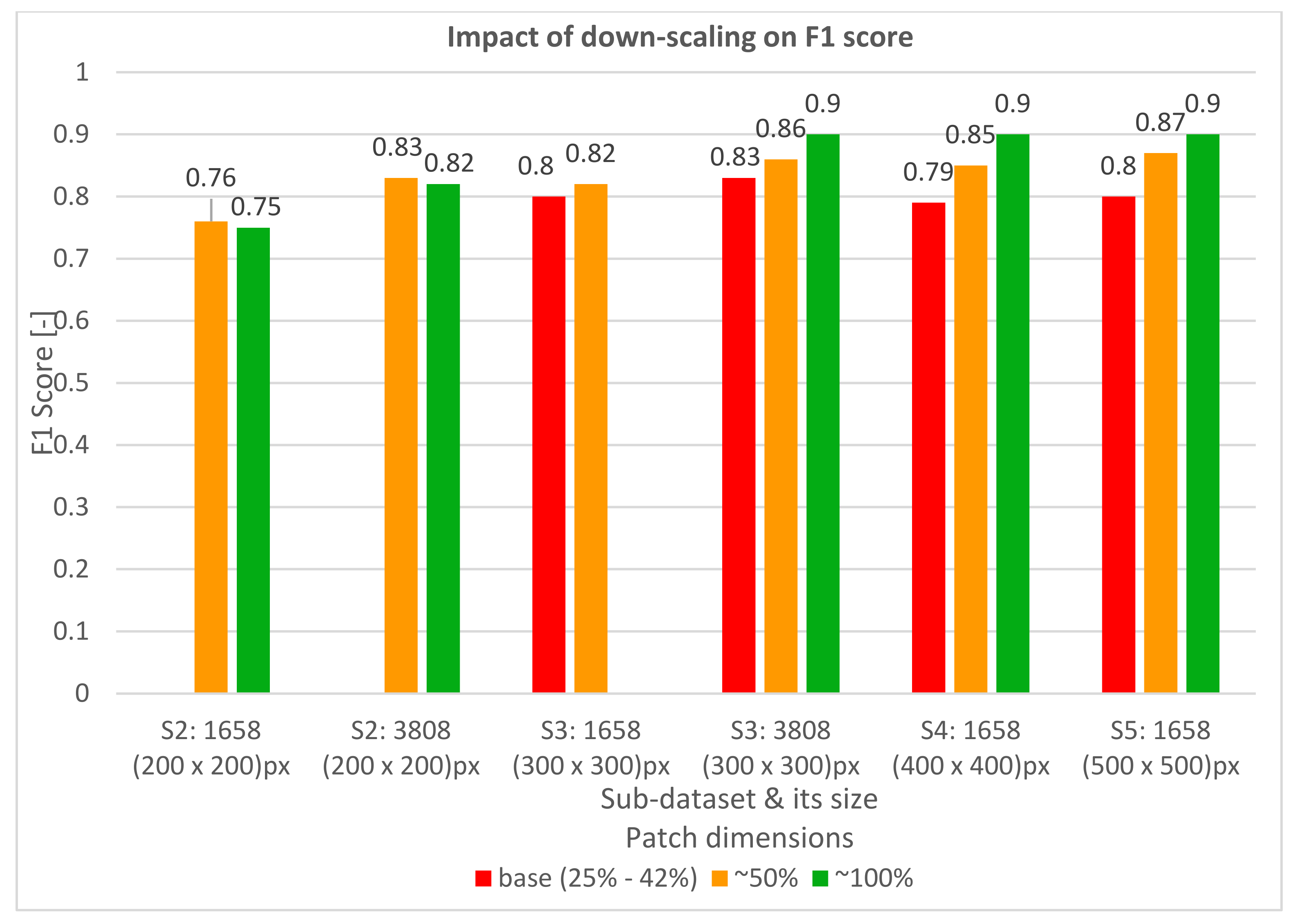
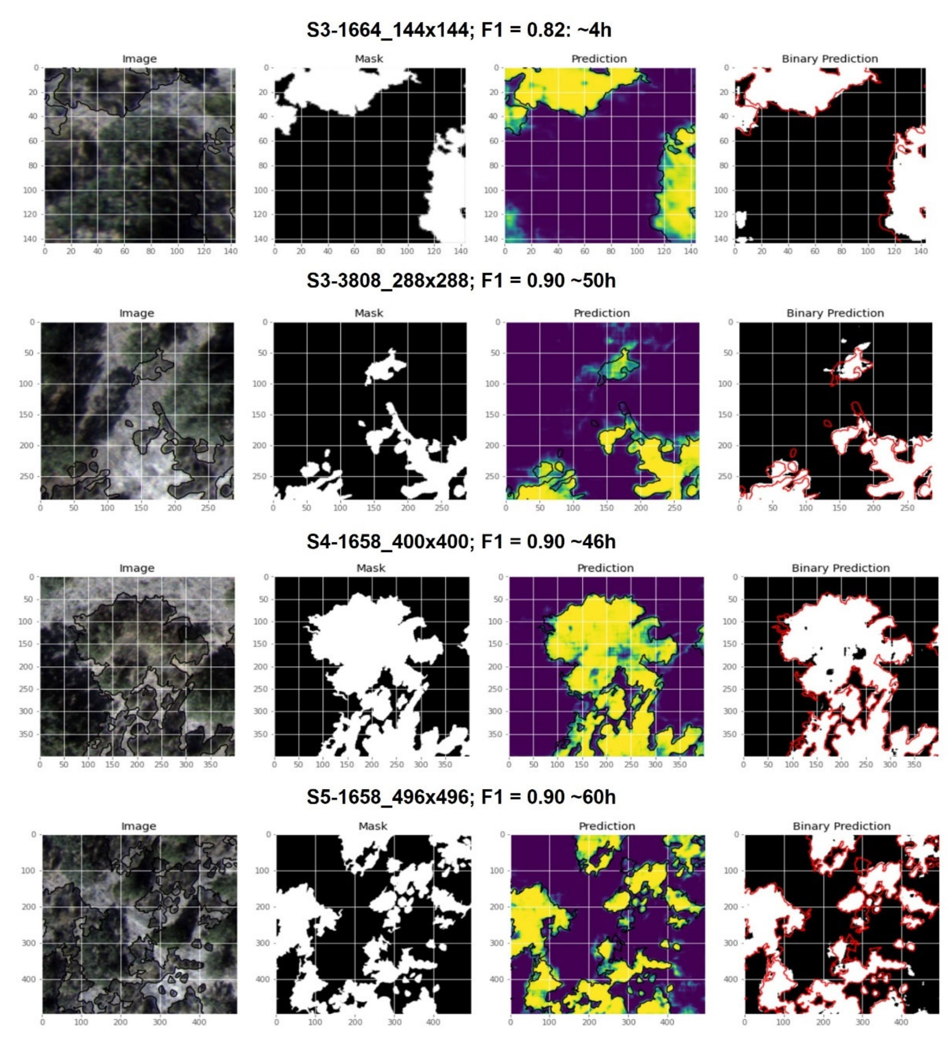
3.1.2. Binary Segmentation
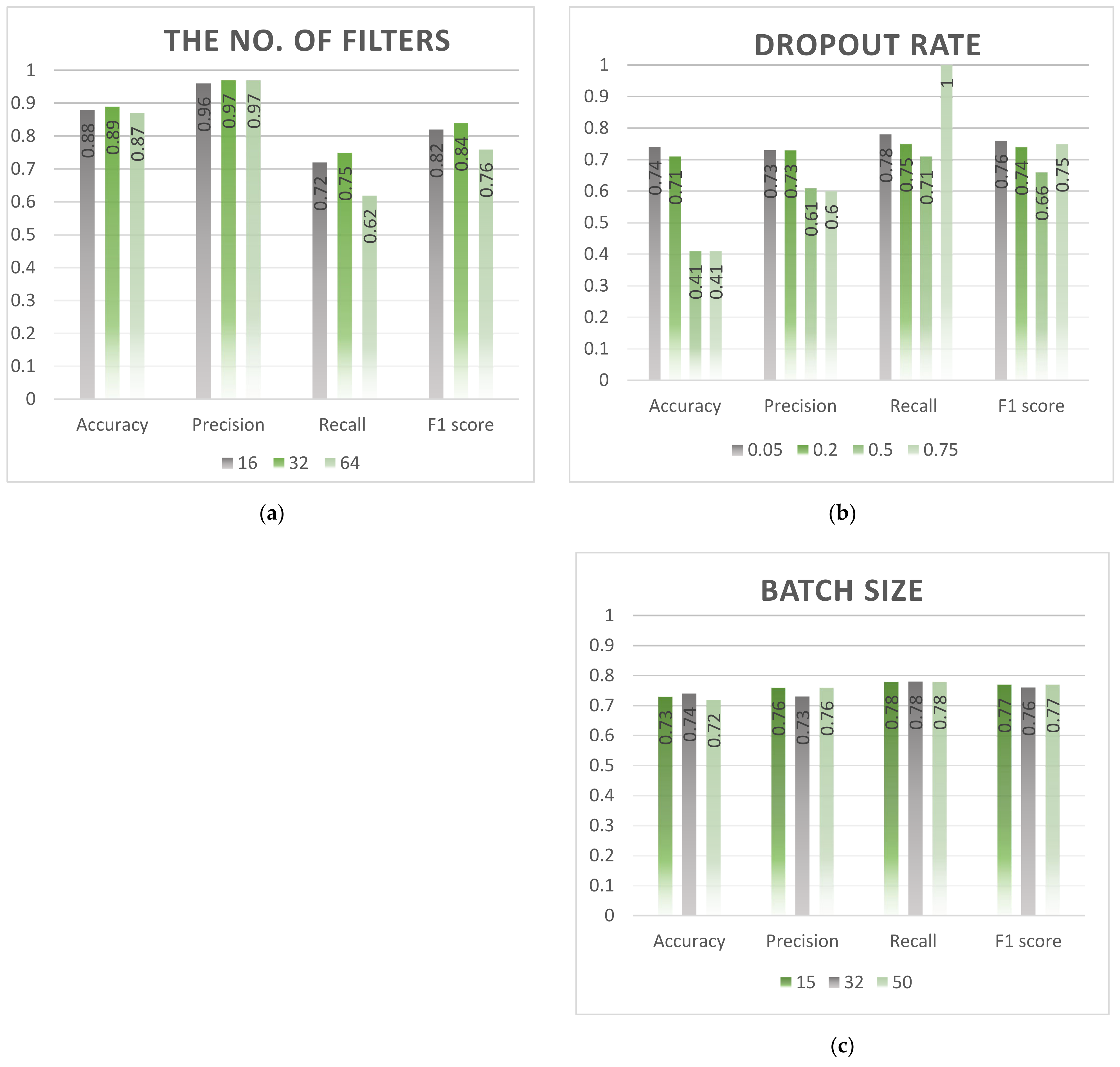
3.1.3. Hyperparameter Tuning
- The initial number of filters: 16, 32 and 64 [50];
3.2. Test Data
4. Discussion
4.1. Preliminary Analysis in the Training Sets
4.1.1. Multi-Class Segmentation
4.1.2. Binary Segmentation
4.1.3. Hyperparameter Tuning
4.2. Test Data
5. Conclusions
- Further enlargement of the datasets, either from more labeled data from spatially and temporally distinct samples, or by employing more data augmentation variants;
- Decreasing labeling incoherency, especially in case of frequently overlapping classes, by using more annotators and stricter rules on how to label mixed classes;
- Alternatively, or in addition to the previous point, reduce the demands on precise segmentation and allow a less precise approach to labeling, e.g., selecting random regions of interest (ROI) within the class area, without identifying the exact borders of the class object. This could yield higher volumes of samples and concurrently dramatically reduce labeling time;
- The systematic search of hyperparameters for augmentation and pre-processing techniques suitable for these particular data and tasks. Due to limited computational resources, we could not perform an exhaustive search of hyperparameters, but we noticed their importance in optimizing performance.
Author Contributions
Funding
Institutional Review Board Statement
Informed Consent Statement
Data Availability Statement
Acknowledgments
Conflicts of Interest
References
- Ahmed, B.; Noman, M.A.A. Land cover classification for satellite images based on normalization technique and Artificial Neural Network. In Proceedings of the 2015 International Conference on Computer and Information Engineering (ICCIE), Rajshahi, Bangladesh, 26–27 November 2015; pp. 138–141. [Google Scholar]
- Fröhlich, B.; Bach, E.; Walde, I.; Hese, S.; Schmullius, C.; Denzler, J. Land cover classification of satellite images using contextual information. ISPRS Ann. Photogramm. Remote Sens. Spat. Inf. Sci. 2013, II-3/W1, 1–6. [Google Scholar] [CrossRef] [Green Version]
- Kussul, N.; Lavreniuk, M.; Skakun, S.; Shelestov, A. Deep Learning Classification of Land Cover and Crop Types Using Remote Sensing Data. IEEE Geosci. Remote Sens. Lett. 2017, 14, 778–782. [Google Scholar] [CrossRef]
- Vanjare, A.; Omkar, S.N.; Senthilnath, J. Satellite Image Processing for Land Use and Land Cover Mapping. Int. J. Image Graph. Signal Process. 2014, 6, 18–28. [Google Scholar] [CrossRef]
- Matese, A.; Toscano, P.; Di Gennaro, S.F.; Genesio, L.; Vaccari, F.P.; Primicerio, J.; Belli, C.; Zaldei, A.; Bianconi, R.; Gioli, B. Intercomparison of UAV, Aircraft and Satellite Remote Sensing Platforms for Precision Viticulture. Remote Sens. 2015, 7, 2971–2990. [Google Scholar] [CrossRef] [Green Version]
- Pérez-Rodríguez, L.A.; Quintano, C.; Marcos, E.; Suarez-Seoane, S.; Calvo, L.; Fernández-Manso, A. Evaluation of Prescribed Fires from Unmanned Aerial Vehicles (UAVs) Imagery and Machine Learning Algorithms. Remote Sens. 2020, 12, 1295. [Google Scholar] [CrossRef] [Green Version]
- Getzin, S.; Wiegand, K.; Schöning, I. Assessing biodiversity in forests using very high-resolution images and unmanned aerial vehicles. Methods Ecol. Evol. 2012, 3, 397–404. [Google Scholar] [CrossRef]
- Mangewa, L.J.; Ndakidemi, P.A.; Munishi, L.K. Integrating UAV Technology in an Ecological Monitoring System for Community Wildlife Management Areas in Tanzania. Sustainability 2019, 11, 6116. [Google Scholar] [CrossRef] [Green Version]
- Csillik, O.; Cherbini, J.; Johnson, R.; Lyons, A.; Kelly, M. Identification of Citrus Trees from Unmanned Aerial Vehicle Imagery Using Convolutional Neural Networks. Drones 2018, 2, 39. [Google Scholar] [CrossRef] [Green Version]
- Kinaneva, D.; Hristov, G.; Raychev, J.; Zahariev, P. Early Forest Fire Detection Using Drones and Artificial Intelligence. In Proceedings of the 2019 42nd International Convention on Information and Communication Technology, Electronics and Microelectronics (MIPRO), Opatija, Croatia, 20–24 May 2019; pp. 1060–1065. [Google Scholar]
- Kerle, N.; Nex, F.; Gerke, M.; Duarte, D.; Vetrivel, A. UAV-Based Structural Damage Mapping: A Review. ISPRS Int. J. Geo-Inf. 2019, 9, 14. [Google Scholar] [CrossRef] [Green Version]
- Sankey, T.; Donager, J.; McVay, J.; Sankey, J.B. UAV lidar and hyperspectral fusion for forest monitoring in the southwestern USA. Remote Sens. Environ. 2017, 195, 30–43. [Google Scholar] [CrossRef]
- Baena, S.; Moat, J.; Whaley, O.; Boyd, D.S. Identifying species from the air: UAVs and the very high resolution challenge for plant conservation. PLoS ONE 2017, 12, e0188714. [Google Scholar] [CrossRef] [Green Version]
- Malenovský, Z.; Lucieer, A.; King, D.H.; Turnbull, J.D.; Robinson, S.A. Unmanned aircraft system advances health mapping of fragile polar vegetation. Methods Ecol. Evol. 2017, 8, 1842–1857. [Google Scholar] [CrossRef] [Green Version]
- Langford, Z.L.; Kumar, J.; Hoffman, F.M.; Breen, A.L.; Iversen, C.M. Arctic Vegetation Mapping Using Unsupervised Training Datasets and Convolutional Neural Networks. Remote Sens. 2019, 11, 69. [Google Scholar] [CrossRef] [Green Version]
- Lopatin, J.; Fassnacht, F.E.; Kattenborn, T.; Schmidtlein, S. Mapping plant species in mixed grassland communities using close range imaging spectroscopy. Remote Sens. Environ. 2017, 201, 12–23. [Google Scholar] [CrossRef]
- Cao, J.; Leng, W.; Liu, K.; Liu, L.; He, Z.; Zhu, Y. Object-Based Mangrove Species Classification Using Unmanned Aerial Vehicle Hyperspectral Images and Digital Surface Models. Remote Sens. 2018, 10, 89. [Google Scholar] [CrossRef] [Green Version]
- Sladojevic, S.; Arsenovic, M.; Anderla, A.; Culibrk, D.; Stefanovic, D. Deep Neural Networks Based Recognition of Plant Diseases by Leaf Image Classification. Available online: https://www.hindawi.com/journals/cin/2016/3289801/ (accessed on 26 December 2020).
- Guirado, E.; Tabik, S.; Alcaraz-Segura, D.; Cabello, J.; Herrera, F. Deep-Learning Convolutional Neural Networks for Scattered Shrub Detection with Google Earth Imagery. arXiv 2017, arXiv:1706.00917. Available online: http://arxiv.org/abs/1706.00917 (accessed on 23 December 2020).
- Ayhan, B.; Kwan, C. Tree, Shrub, and Grass Classification Using Only RGB Images. Remote Sens. 2020, 12, 1333. [Google Scholar] [CrossRef] [Green Version]
- Hellesen, T.; Matikainen, L. An Object-Based Approach for Mapping Shrub and Tree Cover on Grassland Habitats by Use of LiDAR and CIR Orthoimages. Remote Sens. 2013, 5, 558–583. [Google Scholar] [CrossRef] [Green Version]
- Lopatin, J.; Dolos, K.; Kattenborn, T.; Fassnacht, F.E. How canopy shadow affects invasive plant species classification in high spatial resolution remote sensing. Remote Sens. Ecol. Conserv. 2019, 5, 302–317. [Google Scholar] [CrossRef]
- Zhou, Q.; Yang, W.; Gao, G.; Ou, W.; Lu, H.; Chen, J.; Latecki, L.J. Multi-scale deep context convolutional neural networks for semantic segmentation. World Wide Web 2019, 22, 555–570. [Google Scholar] [CrossRef]
- Volpi, M.; Tuia, D. Dense Semantic Labeling of Subdecimeter Resolution Images With Convolutional Neural Networks. IEEE Trans. Geosci. Remote Sens. 2017, 55, 881–893. [Google Scholar] [CrossRef] [Green Version]
- Wen, D.; Huang, X.; Liu, H.; Liao, W.; Zhang, L. Semantic classification of urban trees using very high resolution satellite imagery. IEEE J. Sel. Top. Earth Obs. Remote Sens. 2017, 10, 1413–1424. [Google Scholar] [CrossRef]
- Paisitkriangkrai, S.; Sherrah, J.; Janney, P.; Van Den Hengel, A. Semantic labeling of aerial and satellite imagery. IEEE J. Sel. Top. Appl. Earth Obs. Remote Sens. 2016, 9, 2868–2881. [Google Scholar] [CrossRef]
- Yu, C.; Wang, J.; Peng, C.; Gao, C.; Yu, G.; Sang, N. Learning a Discriminative Feature Network for Semantic Segmentation. In Proceedings of the 2018 IEEE/CVF Conference on Computer Vision and Pattern Recognition, Salt Lake City, UT, USA, 18–23 June 2018; pp. 1857–1866. [Google Scholar]
- Chen, L.-C.; Papandreou, G.; Kokkinos, I.; Murphy, K.; Yuille, A.L. DeepLab: Semantic Image Segmentation with Deep Convolutional Nets, Atrous Convolution, and Fully Connected CRFs. arXiv 2017, arXiv:160600915. Available online: http://arxiv.org/abs/1606.00915 (accessed on 27 December 2020). [CrossRef] [Green Version]
- Li, R.; Liu, W.; Yang, L.; Sun, S.; Hu, W.; Zhang, F.; Li, W. DeepUNet: A Deep Fully Convolutional Network for Pixel-Level Sea-Land Segmentation. IEEE J. Sel. Top. Appl. Earth Obs. Remote Sens. 2018, 11, 3954–3962. [Google Scholar] [CrossRef] [Green Version]
- Long, J.; Shelhamer, E.; Darrell, T. Fully Convolutional Networks for Semantic Segmentation. arXiv 2015, arXiv:1411.4038. Available online: http://arxiv.org/abs/1411.4038 (accessed on 2 November 2020).
- Badrinarayanan, V.; Kendall, A.; Cipolla, R. SegNet: A Deep Convolutional Encoder-Decoder Architecture for Image Segmentation. arXiv 2016, arXiv:151100561. Available online: http://arxiv.org/abs/1511.00561 (accessed on 27 December 2020). [CrossRef]
- Ronneberger, O.; Fischer, P.; Brox, T. U-Net: Convolutional Networks for Biomedical Image Segmentation. arXiv 2015, arXiv:150504597. Available online: http://arxiv.org/abs/1505.04597 (accessed on 13 October 2020).
- Stoian, A.; Poulain, V.; Inglada, J.; Poughon, V.; Derksen, D. Land Cover Maps Production with High Resolution Satellite Image Time Series and Convolutional Neural Networks: Adaptations and Limits for Operational Systems. Remote Sens. 2019, 11, 1986. [Google Scholar] [CrossRef] [Green Version]
- Mahdianpari, M.; Salehi, B.; Rezaee, M.; Mohammadimanesh, F.; Zhang, Y. Very Deep Convolutional Neural Networks for Complex Land Cover Mapping Using Multispectral Remote Sensing Imagery. Remote Sens. 2018, 10, 1119. [Google Scholar] [CrossRef] [Green Version]
- Hung, C.; Xu, Z.; Sukkarieh, S. Feature Learning Based Approach for Weed Classification Using High Resolution Aerial Images from a Digital Camera Mounted on a UAV. Remote Sens. 2014, 6, 12037–12054. [Google Scholar] [CrossRef] [Green Version]
- Ashapure, A.; Jung, J.; Chang, A.; Oh, S.; Maeda, M.; Landivar, J. A Comparative Study of RGB and Multispectral Sensor-Based Cotton Canopy Cover Modelling Using Multi-Temporal UAS Data. Remote Sens. 2019, 11, 2757. [Google Scholar] [CrossRef] [Green Version]
- Solórzano, J.V.; Mas, J.F.; Gao, Y.; Gallardo-Cruz, J.A. Land Use Land Cover Classification with U-Net: Advantages of Combining Sentinel-1 and Sentinel-2 Imagery. Remote Sens. 2021, 13, 3600. [Google Scholar] [CrossRef]
- Korznikov, K.A.; Kislov, D.E.; Altman, J.; Doležal, J.; Vozmishcheva, A.S.; Krestov, P.V. Using U-Net-Like Deep Convolutional Neural Networks for Precise Tree Recognition in Very High Resolution RGB (Red, Green, Blue) Satellite Images. Forests 2021, 12, 66. [Google Scholar] [CrossRef]
- Pereira, H.M.; Navarro, L.M. (Eds.) Rewilding European Landscapes; Springer International Publishing: Cham, Switzerland, 2015; ISBN 978-3-319-12038-6. [Google Scholar]
- Pausas, J.G.; Paula, S. Fuel shapes the fire-climate relationship: Evidence from Mediterranean ecosystems: Fuel shapes the fire-climate relationship. Glob. Ecol. Biogeogr. 2012, 21, 1074–1082. [Google Scholar] [CrossRef]
- Fernandes, P.M. Fire-smart management of forest landscapes in the Mediterranean basin under global change. Landsc. Urban Plan. 2013, 110, 175–182. [Google Scholar] [CrossRef] [Green Version]
- Fernández-Manjarrés, J.; Ruiz-Benito, P.; Zavala, M.; Camarero, J.; Pulido, F.; Proença, V.; Navarro, L.; Sansilvestri, R.; Granda, E.; Marqués, L.; et al. Forest Adaptation to Climate Change along Steep Ecological Gradients: The Case of the Mediterranean-Temperate Transition in South-Western Europe. Sustainability 2018, 10, 3065. [Google Scholar] [CrossRef] [Green Version]
- Álvarez-Martínez, J.; Gómez-Villar, A.; Lasanta, T. The use of goats grazing to restore pastures invaded by shrubs and avoid desertification: A preliminary case study in the Spanish Cantabrian Mountains. Degrad. Dev. 2016, 27, 3–13. [Google Scholar] [CrossRef]
- Silva, J.S.; Moreira, F.; Vaz, P.; Catry, F.; Godinho-Ferreira, P. Assessing the relative fire proneness of different forest types in Portugal. Plant Biosyst.-Int. J. Deal. Asp. Plant Biol. 2009, 143, 597–608. [Google Scholar] [CrossRef]
- Cruz, Ó.; García-Duro, J.; Riveiro, S.F.; García-García, C.; Casal, M.; Reyes, O. Fire Severity Drives the Natural Regeneration of Cytisus scoparius L. (Link) and Salix atrocinerea Brot. Communities and the Germinative Behaviour of These Species. Forests 2020, 11, 124. [Google Scholar] [CrossRef] [Green Version]
- Tarrega, R.; Calvo, L.; Trabaud, L. Effect of High Temperatures on Seed Germination of Two Woody Leguminosae. Vegetatio 1992, 102, 139–147. [Google Scholar] [CrossRef]
- Lovreglio, R.; Meddour-Sahar, O.; Leone, V. Goat grazing as a wildfire prevention tool: A basic review. IForest-Biogeosci. For. 2014, 7, 260–268. [Google Scholar] [CrossRef] [Green Version]
- Reina, G.A.; Panchumarthy, R.; Thakur, S.P.; Bastidas, A.; Bakas, S. Systematic Evaluation of Image Tiling Adverse Effects on Deep Learning Semantic Segmentation. Front. Neurosci. 2020, 14, 65. [Google Scholar] [CrossRef] [PubMed]
- Rakhlin, A.; Davydow, A.; Nikolenko, S. Land Cover Classification from Satellite Imagery with U-Net and Lovász-Softmax Loss. In Proceedings of the 2018 IEEE/CVF Conference on Computer Vision and Pattern Recognition Workshops (CVPRW), Salt Lake City, UT, USA, 18–22 June 2018; pp. 257–2574. [Google Scholar]
- Zhang, P.; Ke, Y.; Zhang, Z.; Wang, M.; Li, P.; Zhang, S. Urban Land Use and Land Cover Classification Using Novel Deep Learning Models Based on High Spatial Resolution Satellite Imagery. Sensors 2018, 18, 3717. [Google Scholar] [CrossRef] [Green Version]
- Zhang, F.; Du, B.; Zhang, L. Saliency-Guided Unsupervised Feature Learning for Scene Classification. IEEE Trans. Geosci. Remote Sens. 2015, 53, 2175–2184. [Google Scholar] [CrossRef]
- Bengio, Y. Practical Recommendations for Gradient-Based Training of Deep Architectures. arXiv 2012, arXiv:12065533. Available online: http://arxiv.org/abs/1206.5533 (accessed on 14 December 2020).
- Keskar, N.S.; Mudigere, D.; Nocedal, J.; Smelyanskiy, M.; Tang, P.T.P. On Large-Batch Training for Deep Learning: Generalization Gap and Sharp Minima. arXiv 2017, arXiv:160904836. Available online: http://arxiv.org/abs/1609.04836 (accessed on 14 December 2020).
- Masters, D.; Luschi, C. Revisiting Small Batch Training for Deep Neural Networks. arXiv 2018, arXiv:180407612. Available online: http://arxiv.org/abs/1804.07612 (accessed on 9 November 2020).
- Zheng, L.; Zhao, Y.; Wang, S.; Wang, J.; Tian, Q. Good Practice in CNN Feature Transfer. arXiv 2016, arXiv:160400133. Available online: http://arxiv.org/abs/1604.00133 (accessed on 2 December 2020).
- Kattenborn, T.; Eichel, J.; Wiser, S.; Burrows, L.; Fassnacht, F.E.; Schmidtlein, S. Convolutional Neural Networks accurately predict cover fractions of plant species and communities in Unmanned Aerial Vehicle imagery. Remote Sens. Ecol. Conserv. 2020, 6, 472–486. [Google Scholar] [CrossRef] [Green Version]
- Zhang, W.; Tang, P.; Zhao, L. Remote Sensing Image Scene Classification Using CNN-CapsNet. Remote Sens. 2019, 11, 494. [Google Scholar] [CrossRef] [Green Version]
- Müllerová, J.; Brůna, J.; Bartaloš, T.; Dvořák, P.; Vítková, M.; Pyšek, P. Timing Is Important: Unmanned Aircraft vs. Satellite Imagery in Plant Invasion Monitoring. Front. Plant Sci. 2017, 8, 887. [Google Scholar] [CrossRef] [Green Version]
- Audebert, N.; Le Saux, B.; Lefèvre, S. Beyond RGB: Very high resolution urban remote sensing with multimodal deep networks. ISPRS J. Photogramm. Remote Sens. 2018, 140, 20–32. [Google Scholar] [CrossRef] [Green Version]
- Iglovikov, V.; Mushinskiy, S.; Osin, V. Satellite Imagery Feature Detection using Deep Convolutional Neural Network: A Kaggle Competition. arXiv 2017, arXiv:170606169. Available online: http://arxiv.org/abs/1706.06169 (accessed on 2 December 2020).


| Class | Shrubs | Trees | Shadows | Rocks |
|---|---|---|---|---|
| Pixel count | 1,746,204 | 4,042,008 | 1,213,720 | 90,313 |
| Pixel share | 20.99% | 48.58% | 14.59% | 1.09% |
| Shrubs | Trees | Shadows | Rocks | |
|---|---|---|---|---|
| Accuracy | 0.46 | 0.79 | 0.90 | 0.99 |
| Precision | 0.23 | 0.83 | 0.77 | 0.72 |
| Recall | 0.96 | 0.83 | 0.63 | 0.18 |
| F1 Score | 0.31 | 0.83 | 0.69 | 0.29 |
| Reference | ||||
|---|---|---|---|---|
| Classified | Shrubs | Trees | Shadows | Rocks |
| Shrubs | 28.44% | 1.87% | 0.08% | 0.00% |
| Trees | 6.83% | 43.69% | 0.89% | 0.00% |
| Shadows | 5.17% | 2.15% | 9.52% | 0.00% |
| Rocks | 0.74% | 0.05% | 0.08% | 0.48% |
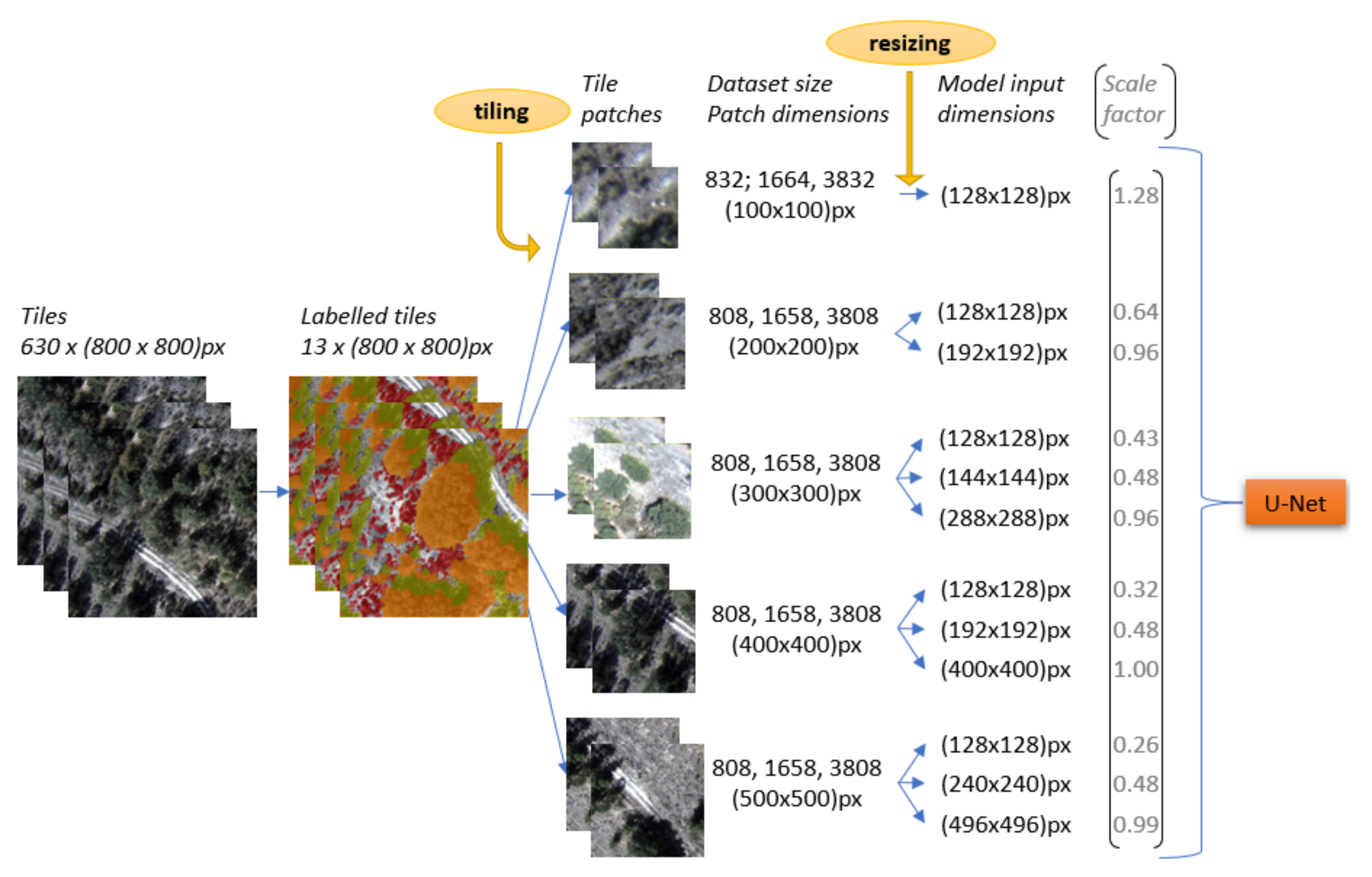
| No. | Class | Dataset Size | Patch Dimensions (px) | Model Input Dimensions (px) |
|---|---|---|---|---|
| 1 | Shrubs (augmented) | 808 | 200 × 200 | 128 × 128 |
| 2 | 1658 | 128 × 128 | ||
| 3 | 1658 | 192 × 192 | ||
| 4 | 3808 | 128 × 128 | ||
| 5 | 3808 | 192 × 192 | ||
| 6 | 808 | 300 × 300 | 128 × 128 | |
| 7 | 1658 | 128 × 128 | ||
| 8 | 1658 | 144 × 144 | ||
| 9 | 3808 | 128 × 128 | ||
| 10 | 3808 | 144 × 144 | ||
| 11 | 3808 | 288 × 288 | ||
| 12 | 808 | 400 × 400 | 128 × 128 | |
| 13 | 1658 | 128 × 128 | ||
| 14 | 1658 | 192 × 192 | ||
| 15 | 1658 | 400 × 400 | ||
| 16 | 3808 | 128 × 128 | ||
| 17 | 808 | 500 × 500 | 128 × 128 | |
| 18 | 1658 | 128 × 128 | ||
| 19 | 1658 | 240 × 240 | ||
| 20 | 1658 | 496 × 496 | ||
| 21 | 3808 | 128 × 128 |
| Patch Size (px) | Patch Size (m) | Scale (cm/1 px) | Model Input Size (px) | Scale (cm/1 px) | Model Input Size (px) | Scale (cm/1 px) | Model Input Size (px) | Scale (cm/1 px) |
|---|---|---|---|---|---|---|---|---|
| 800 | 50.00 | 6.25 | - | - | - | - | - | - |
| 500 | 31.25 | 128 | 24.41 | 240 | 13.02 | 496 | 6.30 | |
| 400 | 25.00 | 128 | 19.53 | 192 | 13.02 | 400 | 6.25 | |
| 300 | 18.75 | 128 | 14.65 | 144 | 13.02 | 288 | 6.51 | |
| 200 | 12.50 | 128 | 9.77 | 192 | 6.51 | - | - | |
| 100 | 6.25 | 128 | 4.88 | - | - | - | - |
| Dataset Size | Patch Dimensions (px) | Model Input Dimensions (px) | F1 (-) (Validation Data) | No. of the Test Set | F1 (-) (Test Data) |
|---|---|---|---|---|---|
| 3808 | 200 × 200 (S2) | 192 × 192 | 0.82 | 1 | 0.60 |
| 2 | 0.64 | ||||
| 3 | 0.63 | ||||
| 300 × 300 (S3) | 288 × 288 | 0.90 | 1 | 0.77 | |
| 2 | 0.76 | ||||
| 3 | 0.62 | ||||
| 1658 | 400 × 400 (S4) | 400 × 400 | 0.90 | 1 | 0.69 |
| 2 | 0.68 | ||||
| 3 | 0.61 | ||||
| 500 × 500 (S5) | 496 × 496 | 0.90 | 1 | 0.67 | |
| 2 | 0.67 | ||||
| 3 | 0.58 |
Publisher’s Note: MDPI stays neutral with regard to jurisdictional claims in published maps and institutional affiliations. |
© 2022 by the authors. Licensee MDPI, Basel, Switzerland. This article is an open access article distributed under the terms and conditions of the Creative Commons Attribution (CC BY) license (https://creativecommons.org/licenses/by/4.0/).
Share and Cite
Trenčanová, B.; Proença, V.; Bernardino, A. Development of Semantic Maps of Vegetation Cover from UAV Images to Support Planning and Management in Fine-Grained Fire-Prone Landscapes. Remote Sens. 2022, 14, 1262. https://doi.org/10.3390/rs14051262
Trenčanová B, Proença V, Bernardino A. Development of Semantic Maps of Vegetation Cover from UAV Images to Support Planning and Management in Fine-Grained Fire-Prone Landscapes. Remote Sensing. 2022; 14(5):1262. https://doi.org/10.3390/rs14051262
Chicago/Turabian StyleTrenčanová, Bianka, Vânia Proença, and Alexandre Bernardino. 2022. "Development of Semantic Maps of Vegetation Cover from UAV Images to Support Planning and Management in Fine-Grained Fire-Prone Landscapes" Remote Sensing 14, no. 5: 1262. https://doi.org/10.3390/rs14051262
APA StyleTrenčanová, B., Proença, V., & Bernardino, A. (2022). Development of Semantic Maps of Vegetation Cover from UAV Images to Support Planning and Management in Fine-Grained Fire-Prone Landscapes. Remote Sensing, 14(5), 1262. https://doi.org/10.3390/rs14051262