
Reducing the Residual Topography Phase for the Robust Landscape Deformation Monitoring of Architectural Heritage Sites in Mountain Areas: The Pseudo-Combination SBAS Method


Abstract
:1. Introduction
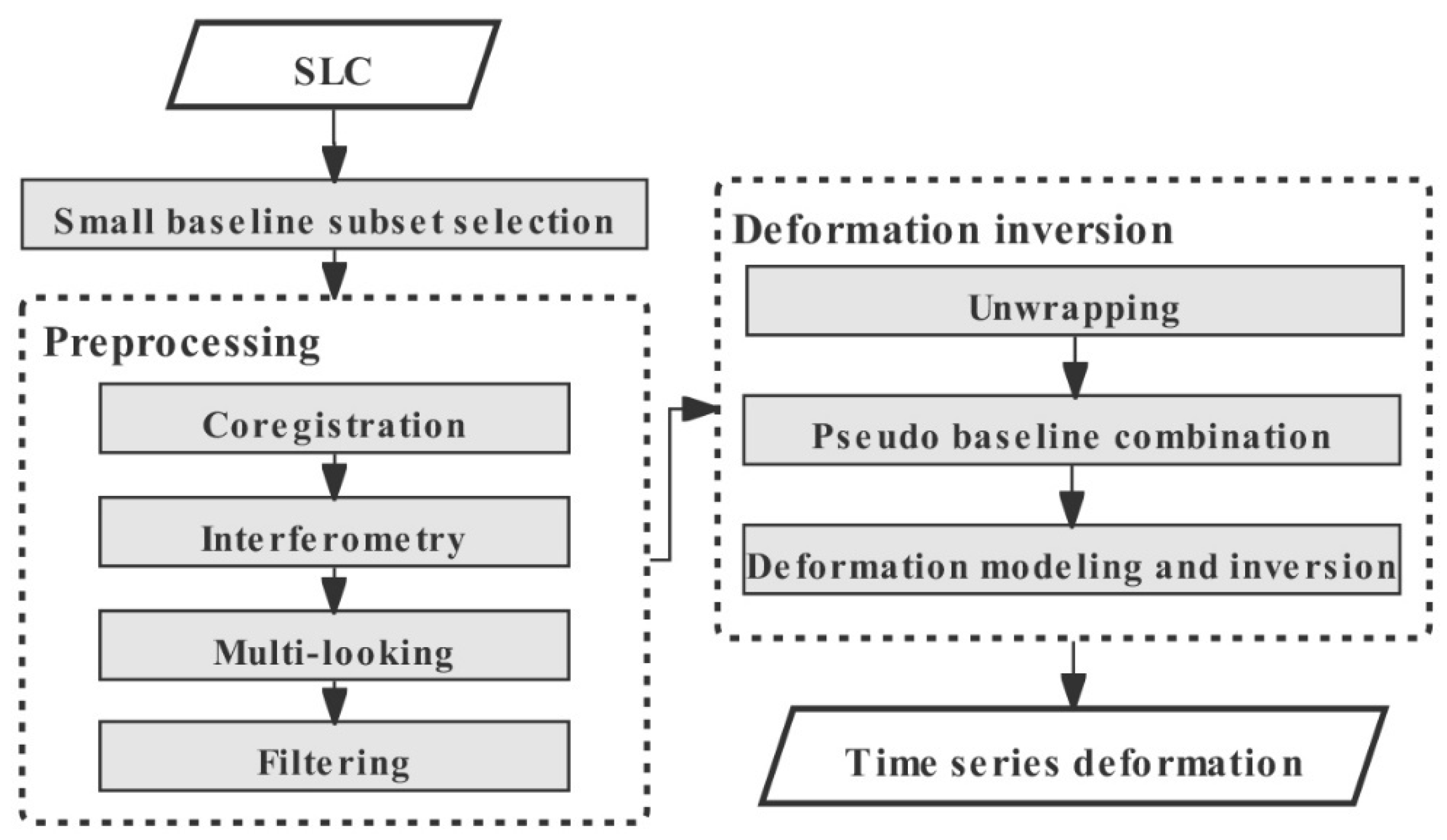
2. Methods
3. Performance Verification
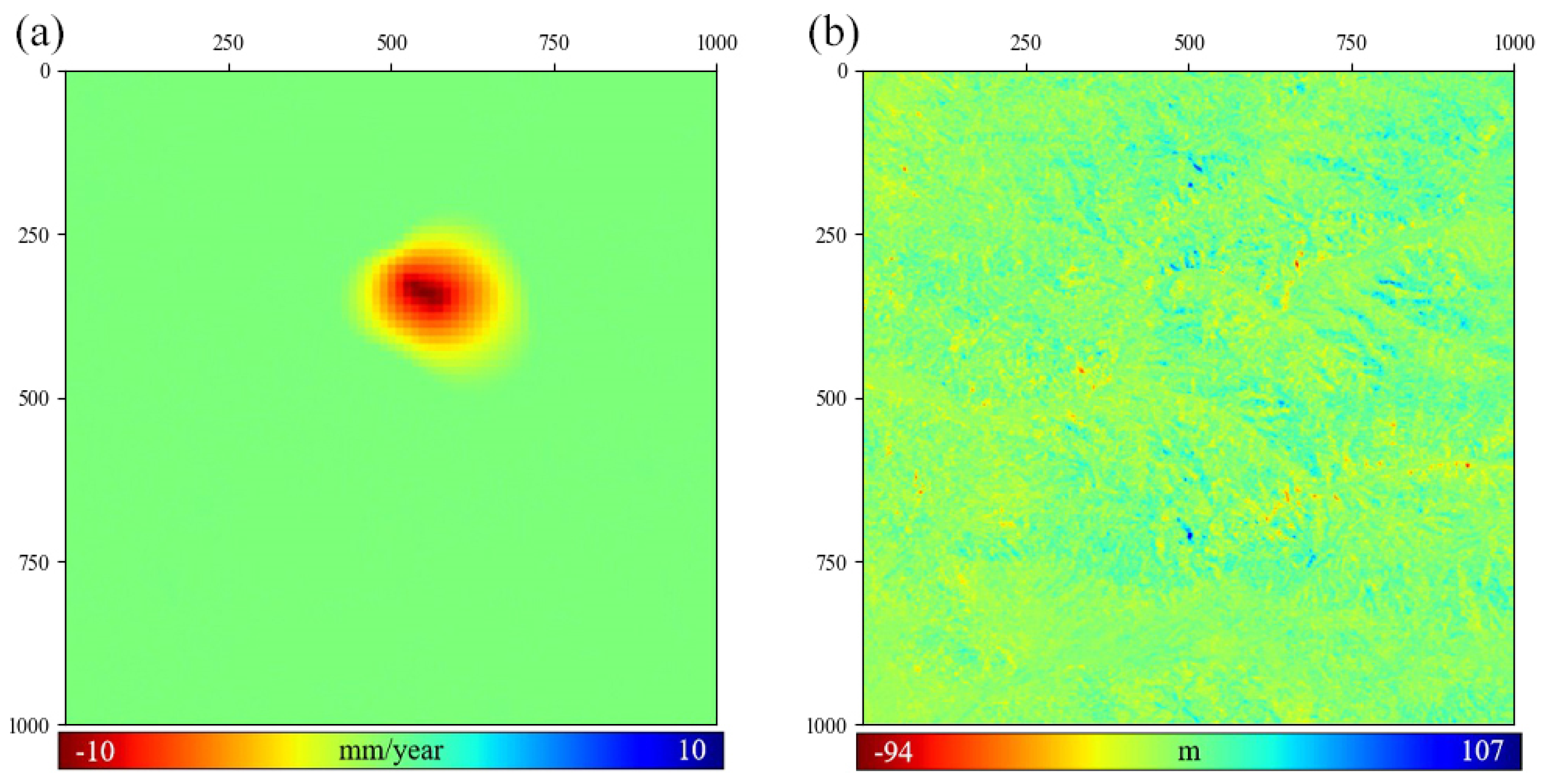
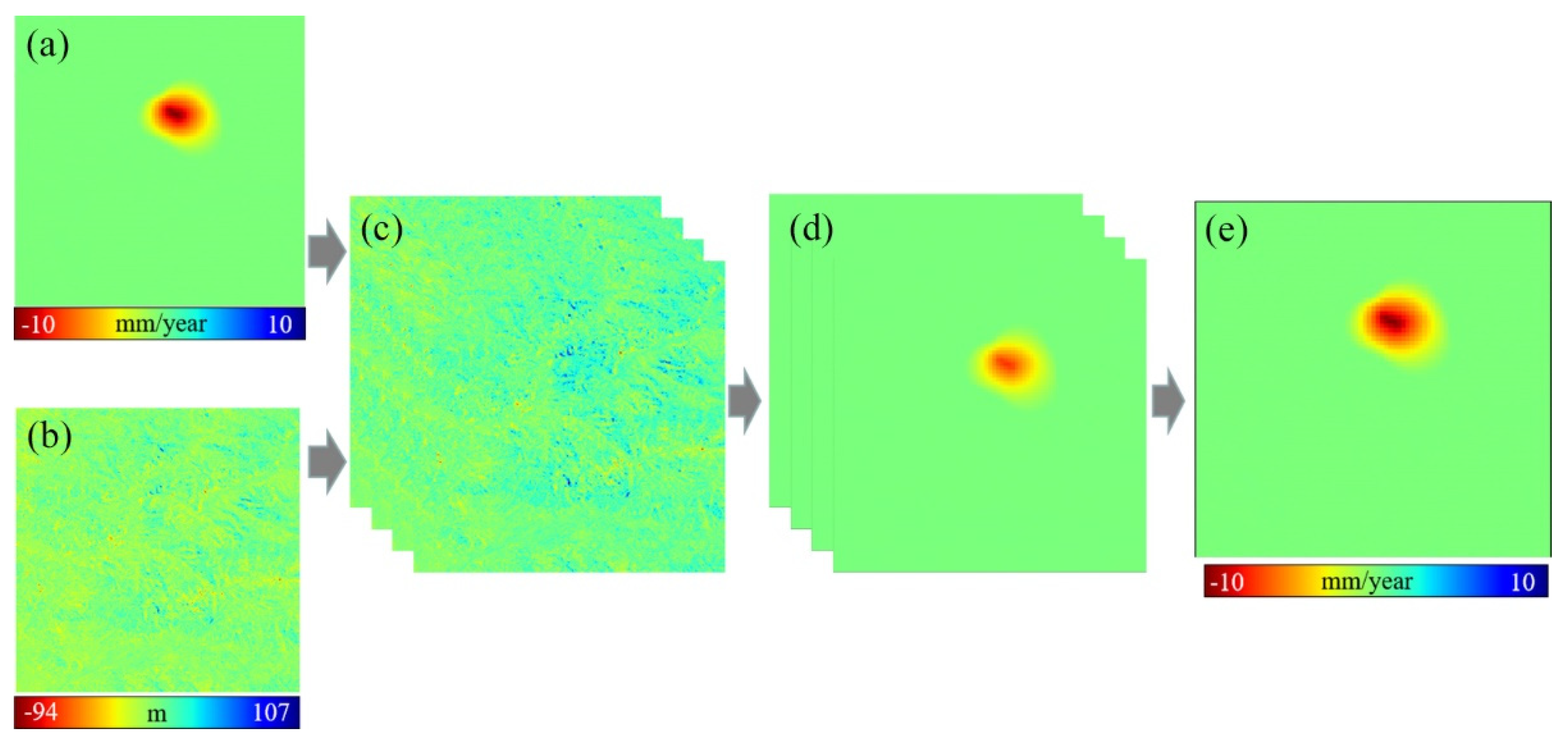
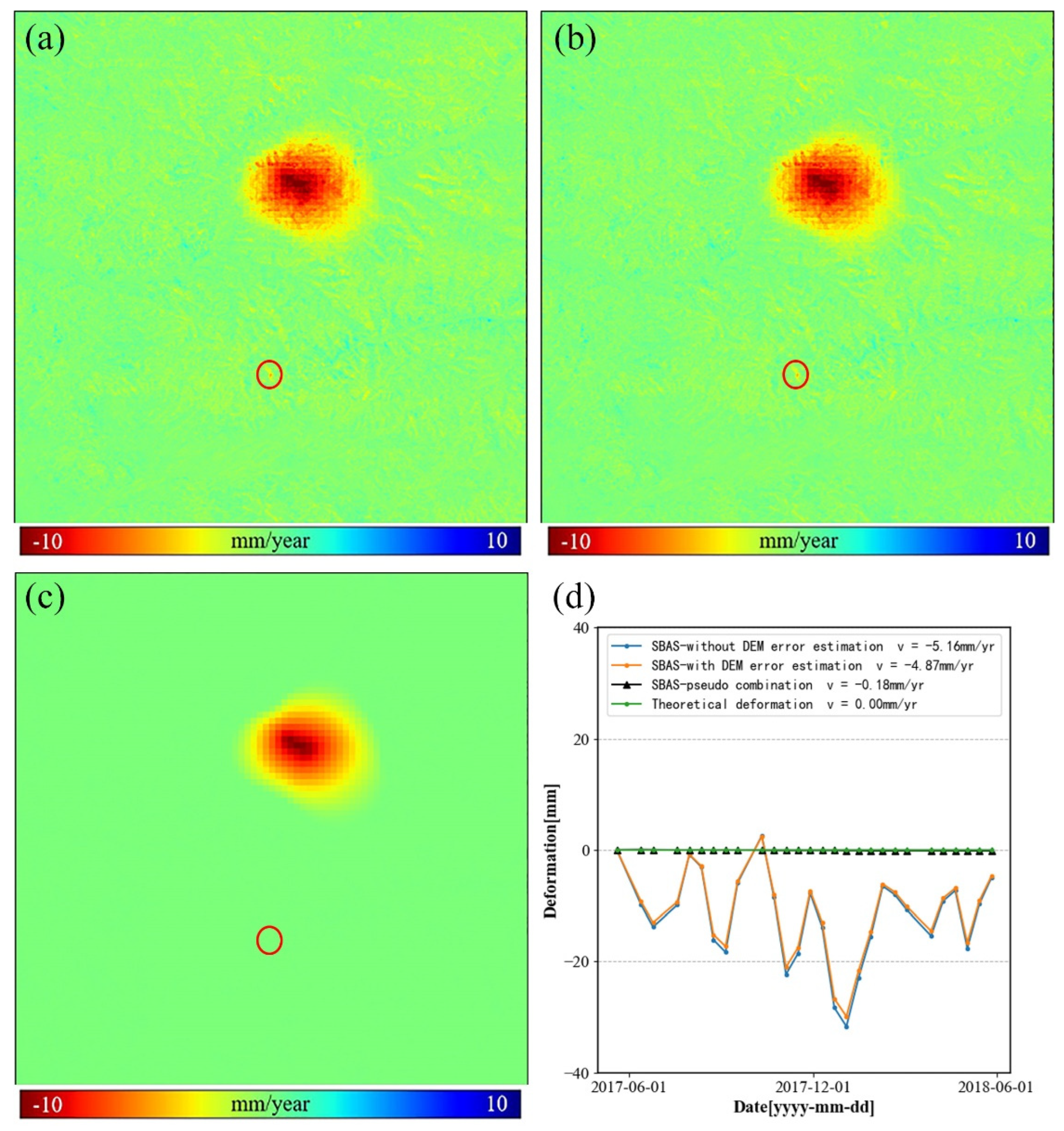
3.1. Performance Verification Using Simulated Data
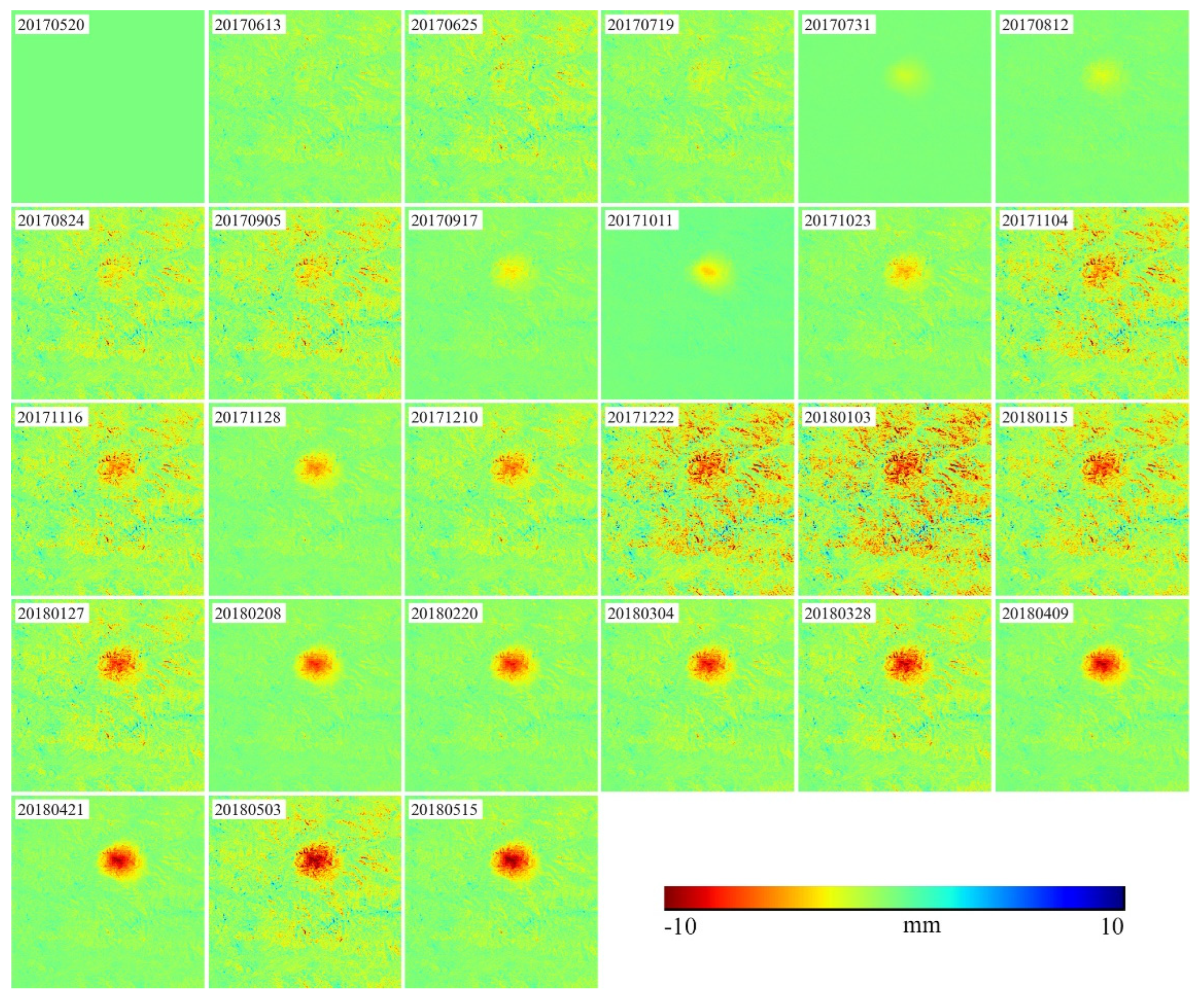
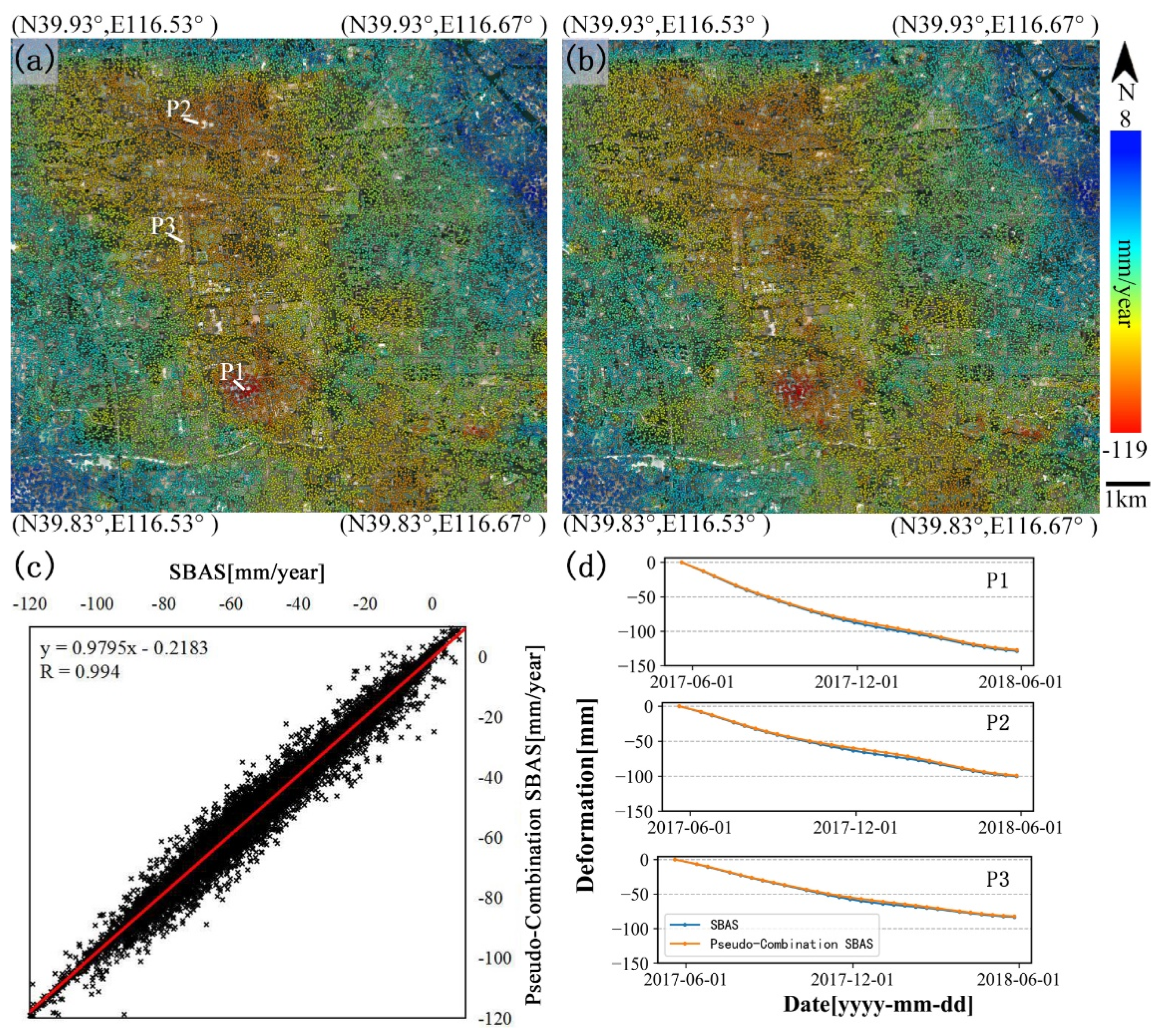
3.2. Performance Verification on Real Data
4. Application to Mountain Area
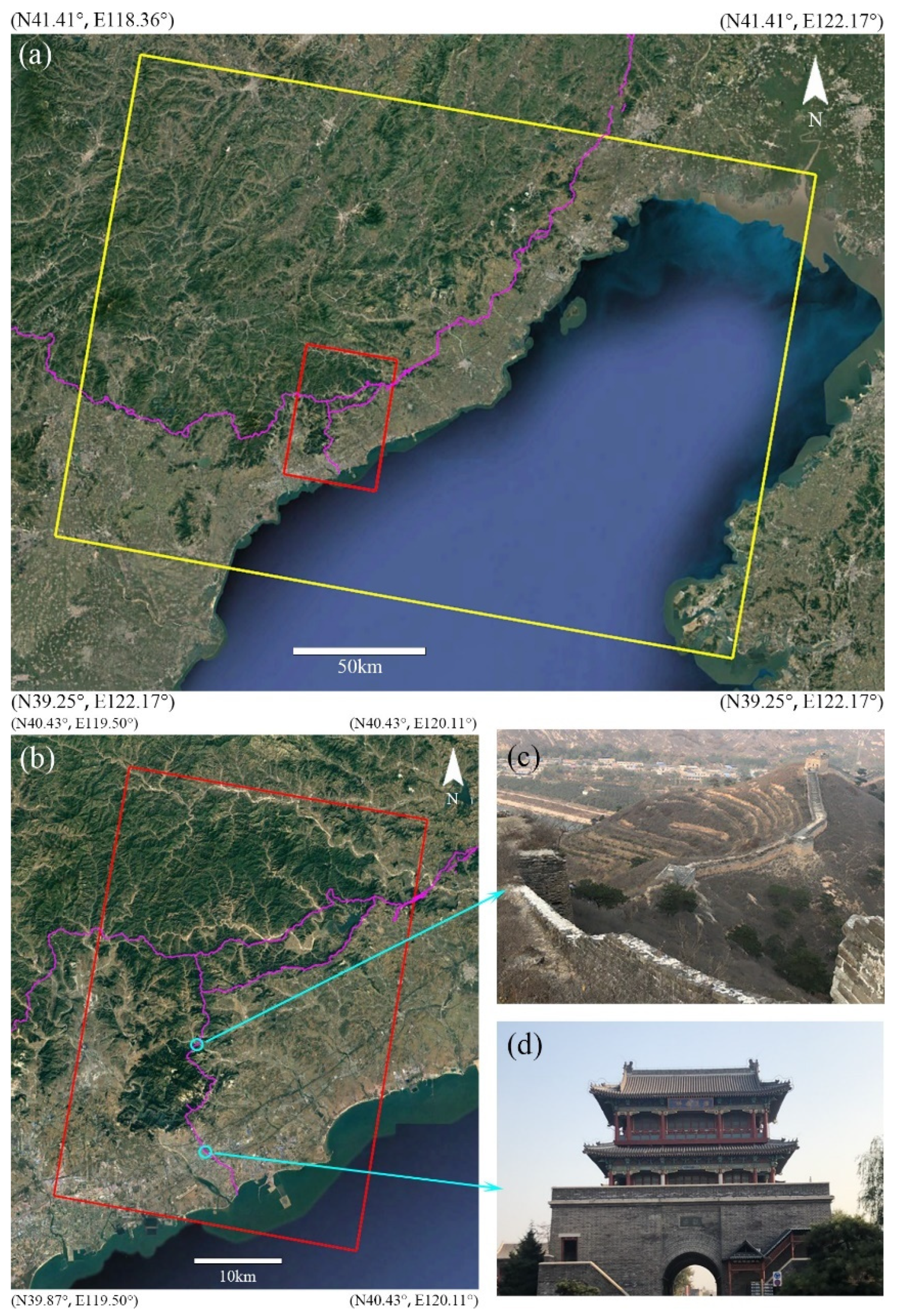
4.1. Study Site
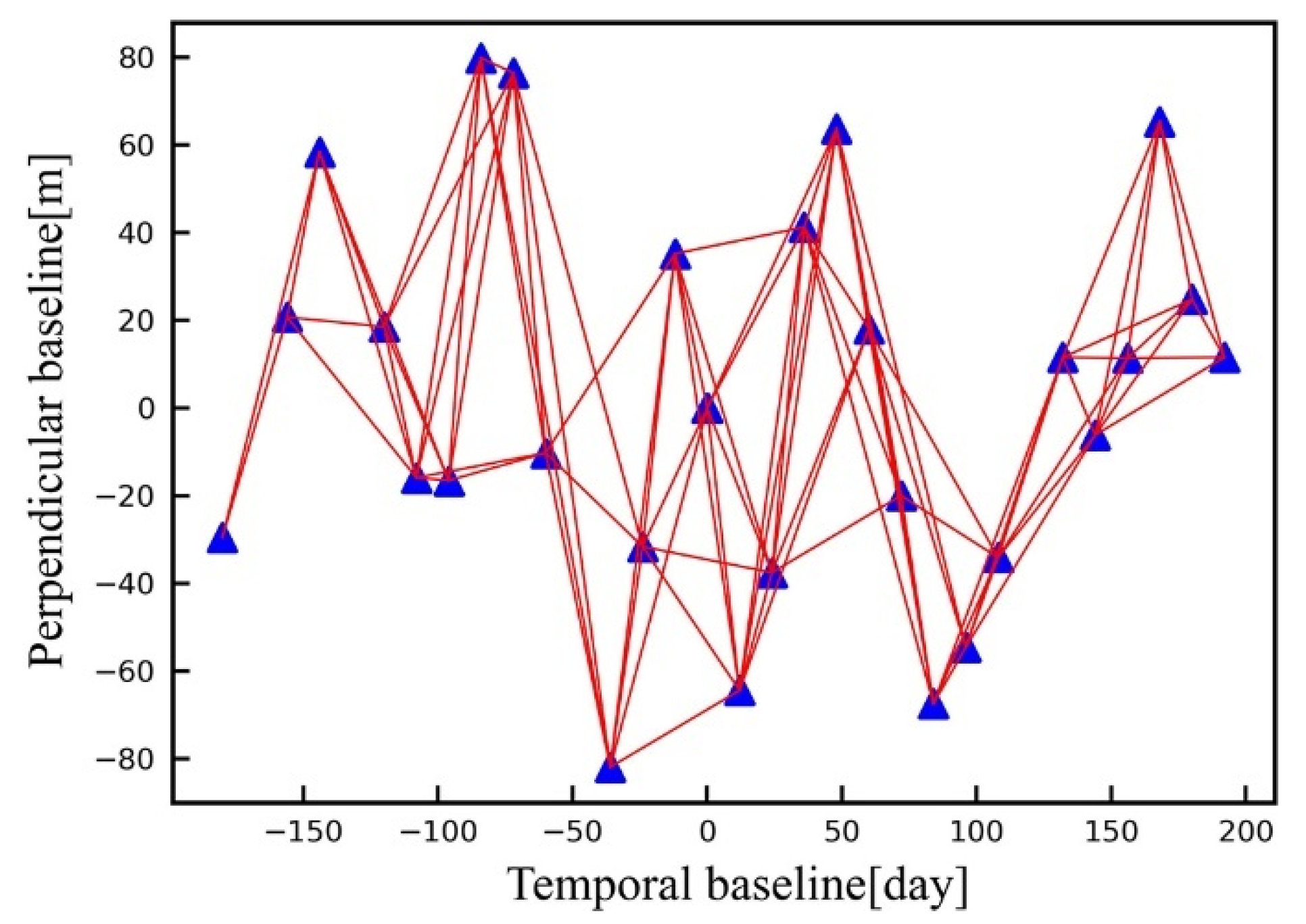
4.2. Data
4.3. Data Processing
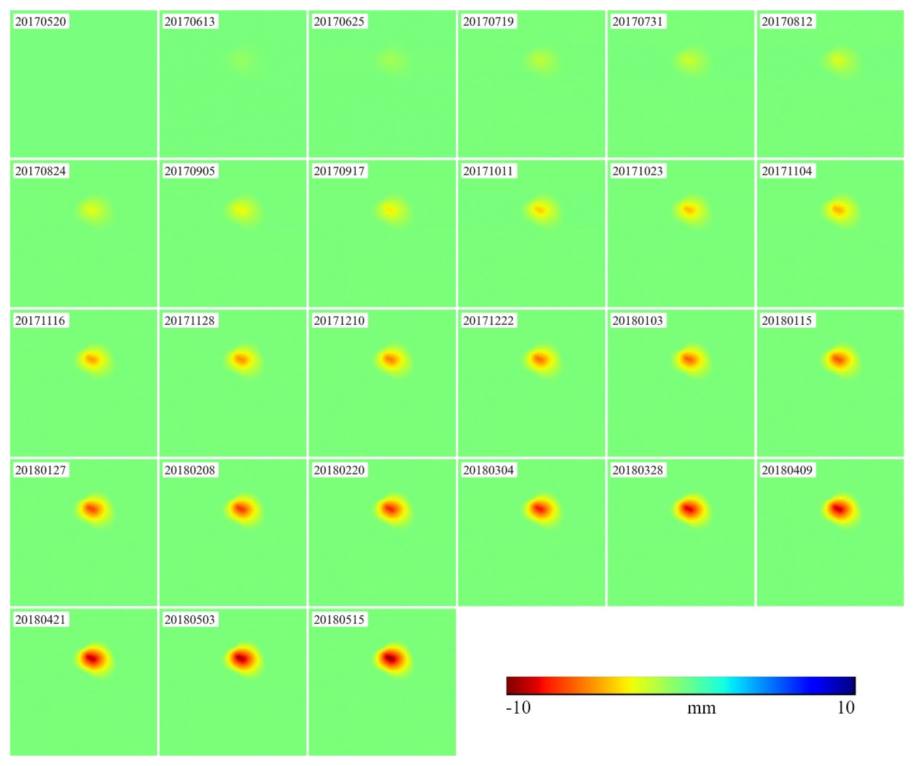
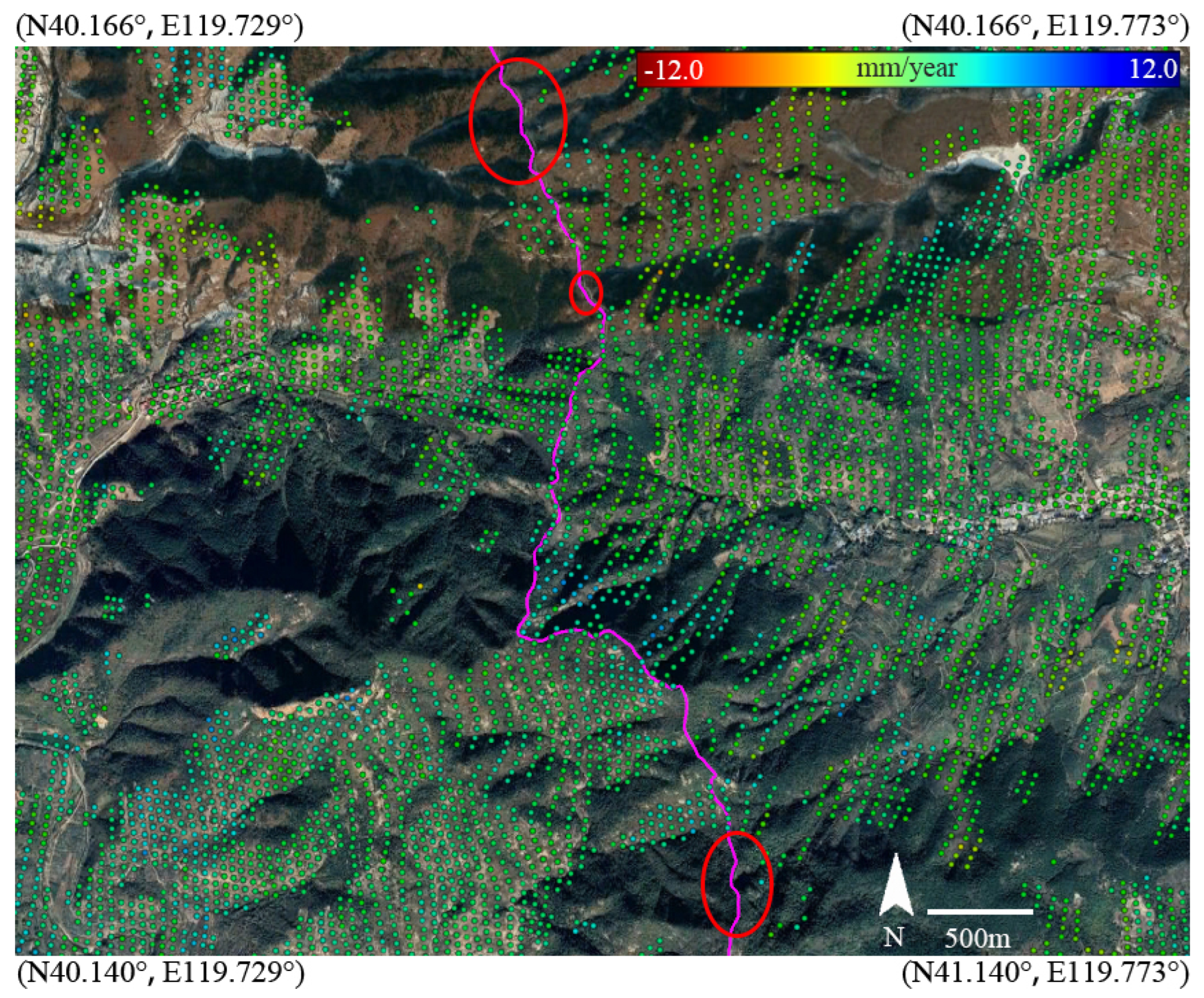
4.4. Deformation Interpretation
5. Discussion
6. Conclusions and Prospects
Author Contributions
Funding
Institutional Review Board Statement
Informed Consent Statement
Data Availability Statement
Acknowledgments
Conflicts of Interest
References
- Gibas-Tracy, D.R. Cost-effective environmental consulting using geographic information systems and remote sensing. Geoscience and Remote Sensing Symposium, 1996. Int. Geosci. Remote Sens. Symp. 1996, 4, 2234–2236. [Google Scholar] [CrossRef]
- Crosse, W. The opportunities and constraints in using cost-effective satellite remote sensing for biodiversity monitoring. Oceans IEEE 2005, 1, 844–849. [Google Scholar] [CrossRef]
- Shinozuka, M.; Ghanem, R.; Houshmand, B.; Mansouri, B. Damage detection in urban areas by SAR imagery. J. Eng. Mech. 2000, 126, 769–777. [Google Scholar] [CrossRef]
- Ma, M.; Chen, J.; Liu, W.; Yang, W. Ship classification and detection based on CNN using GF-3 SAR images. Remote Sens. 2018, 10, 2043. [Google Scholar] [CrossRef] [Green Version]
- Bamler, R.; Hartl, P. Synthetic aperture radar interferometry. Inverse Probl. 1998, 14, R1–R54. [Google Scholar] [CrossRef]
- Jiang, Y.; Xu, Q.; Lu, Z. Landslide Displacement Monitoring by Time Series InSAR Combining PS and DS Targets. Int. Geosci. Remote Sens. Symp. 2020, 1011–1014. [Google Scholar] [CrossRef]
- Horst, T.; Rutten, M.M.; Giesen, N.C.; Hanssen, R.F. Monitoring land subsidence in Yanggon, Myanmar using Sentinel-1 persistent scatterer interferometry and assessment of driving mechanisms. Remote Sens. Environ. 2018, 217, 101–110. [Google Scholar] [CrossRef] [Green Version]
- Milillo, P.; Perissin, D.; Salzer, J.T.; Lundgren, P.; Lacava, G.; Milillo, G.; Serio, C. Monitoring dam structural health from space: Insights from novel InSAR techniques and multi-parametric modeling applied to the Pertusillo dam Basilicata, Italy. Int. J. Appl. Earth Obs. Geoinf. 2016, 52, 221–229. [Google Scholar] [CrossRef]
- Crosetto, M.; Monserrat, O.; Cuevas-Gonzalez, M.; Cuevas-Gonzáleza, M.; Devanthérya, N.; Luzia, G.; Crippab, B. Measuring thermal expansion using X-band persistent scatterer interferometry. ISPRS J. Photogramm. Remote Sens. 2015, 100, 84–91. [Google Scholar] [CrossRef] [Green Version]
- Qin, X.; Li, Q.; Ding, X.; Xie, L.; Wang, C.; Liao, M.; Zhang, L.; Zhang, B.; Xiong, S. A structure knowledge-synthetic aperture radar interferometry integration method for high-precision deformation monitoring and risk identification of sea-crossing bridges. Int. J. Appl. Earth Obs. Geoinf. 2021, 103, 102476. [Google Scholar] [CrossRef]
- Xu, H.; Chen, F.; Zhou, W. A comparative case study of MTInSAR approaches for deformation monitoring of the cultural landscape of the Shanhaiguan section of the Great Wall. Herit. Sci. 2021, 9, 71. [Google Scholar] [CrossRef]
- Bosiljkov, V.; Uranjek, M.; Arni, R.; Bokan-Bosiljkov, V. An integrated diagnostic approach for the assessment of historic masonry structures. J. Cult. Herit. 2010, 11, 239–249. [Google Scholar] [CrossRef]
- Pasek, J.; Gaya, H.P. Numerical simulations of the influence of temperature changes on structural integrity of stone temples in Angkor, Cambodia. Appl. Math. Comput. 2015, 267, 409–418. [Google Scholar] [CrossRef]
- Gigli, G.; Frodella, W.; Mugnai, F.; Tapete, D.; Cigna, F.; Fanti, R.; Intrieri, E.; Lombardi, L. Instability mechanisms affecting cultural heritage sites in the Maltese Archipelago. Nat. Hazards Earth Syst. Sci. 2012, 12, 1883–1903. [Google Scholar] [CrossRef] [Green Version]
- Chen, F.; Xu, H.; Zhou, W.; Deng, W.; Parcharidis, I. Three-dimensional deformation monitoring and simulations for the preventive conservation of architectural heritage: A case study of the Angkor Wat Temple, Cambodia. GIsci. Remote Sens. 2021, 58, 217–234. [Google Scholar] [CrossRef]
- Nuttens, T.; Wulf, A.D.; Deruyter, G.; Stal, C. Deformation monitoring with terrestrial laser scanning: Measurement and processing optimization through experience. Int. Multidiscip. Sci. GeoConf.-SGEM 2012, 707–714. [Google Scholar] [CrossRef]
- Tapete, D.; Cigna, F. Site-specific analysis of deformation patterns on archaeological heritage by satellite radar interferometry. MRS Online Proc. Libr. (OPL) 2012, 1374, 283–295. [Google Scholar] [CrossRef] [Green Version]
- Suziedelyte-Visockiene, J.; Bagdziunaite, R.; Malys, N.; Maliene, V. Close-range photogrammetry enables documentation of environment-induced deformation of architectural heritage. Environ. Eng. Manag. J. 2015, 14, 1371–1381. [Google Scholar] [CrossRef]
- Garziera, R.; Amabili, M.; Collini, L. Structural health monitoring techniques for historical buildings. In Proceedings of the IV Pan American Conference for Non Destructive Testing, Buenos Aires, Argentina, 22–26 October 2007; pp. 1–12. [Google Scholar]
- Sigurdardottir, D.H.; Glisic, B. On-site validation of fiber-optic methods for structural health monitoring: Streicker Bridge. J. Civil Struct. Health Monit. 2015, 5, 529–549. [Google Scholar] [CrossRef]
- Tapete, D.; Fanti, R.; Cecchi, R.; Petrangeli, P.; Casagli, N. Satellite radar interferometry for monitoring and early-stage warning of structural instability in archaeological sites. J. Geophys. Eng. 2012, 9, 10–25. [Google Scholar] [CrossRef]
- Parcharidis, I.; Foumelis, M.; Pavlopoulos, K.; Kourkouli, P. Ground deformation monitoring in cultural heritage areas by time series interferometry: The case of ancient Olympia site (western Greece). Int. Geosci. Remote Sens. Symp. 2010. [Google Scholar]
- Cigna, F.; Lasaponara, R.; Masini, N.; Milillo, P.; Tapete, D. Persistent scatterer interferometry processing of COSMO-SkyMed StripMap HIMAGE time series to depict deformation of the historic centre of Rome, Italy. Remote Sens. 2014, 6, 12593–12618. [Google Scholar] [CrossRef] [Green Version]
- Themistocleous, K.; Cuca, B.; Agapiou, A.; Lysandrou, V.; Tzouvaras, M.; Hadjimitsis, D.; Kyriakides, P.; Kouhartsiouk, D.; Margottini, C.; Spizzichino, D.; et al. The protection of cultural heritage sites from Geo-Hazards: The PROTHEGO project. In Proceedings of the 6th International Conference, EuroMed 2016, Nicosia, Cyprus, October 31–November 5 2016; pp. 91–98. [Google Scholar]
- Chen, F.; Zhou, W.; Xu, H.; Parcharidis, I.; Lin, H.; Fang, C. Space technology facilitates the preventive monitoring and preservation of the Great Wall of the Ming dynasty: A comparative study of the Qingtongxia and Zhangjiakou sections in China. IEEE J. Sel. Top. Appl. Earth Obs. Remote Sens. 2020, 13, 5719–5729. [Google Scholar] [CrossRef]
- Gaber, A.; Darwish, N.; Koch, M. Minimizing the residual topography effect on interferograms to improve DInSAR results: Estimating land subsidence in Port-Said city, Egypt. Remote Sens. 2017, 9, 752. [Google Scholar] [CrossRef] [Green Version]
- Zebker, H.A.; Rosen, P.; Goldstein, R.M.; Gabriel, A.; Werner, C.L. On the derivation of coseismic displacement fields using differential radar interferometry: The Landers earthquake. J. Geophys. Res. 1994, 99, 19617–19634. [Google Scholar] [CrossRef]
- Du, Y.; Zhang, L.; Feng, G.; Lu, Z.; Sun, Q. On the accuracy of topographic residuals retrieved by MTInSAR. IEEE Trans. Geosci. Remote Sens. 2017, 55, 1053–1065. [Google Scholar] [CrossRef]
- Ducret, G.; Doin, M.P.; Grandin, R.; Lasserre, C.; Guillaso, S. Dem corrections before unwrapping in a Small Baseline strategy for InSAR time series analysis. IEEE Geosci Remote Sens. Lett. 2013, 11, 696–700. [Google Scholar] [CrossRef]
- Bayer, B.; Schmidt, D.; Simoni, A. The influence of external digital elevation models on PS-InSAR and SBAS results: Implications for the analysis of deformation signals caused by slow moving landslides in the Northern Apennines (Italy). IEEE Trans. Geosci. Remote Sens. 2017, 55, 2618–2631. [Google Scholar] [CrossRef]
- Ferretti, A.; Prati, C.; Rocca, F. Permanent scatterers in SAR interferometry. IEEE Trans. Geosci. Remote Sens. 2001, 39, 8–20. [Google Scholar] [CrossRef]
- Berardino, P.; Fornaro, G.; Lanari, R. A new algorithm for surface deformation monitoring based on small baseline differential SAR interferograms. IEEE Trans. Geosci. Remote Sens. 2002, 40, 2375–2383. [Google Scholar] [CrossRef] [Green Version]
- Samsonov, S. Topographic correction for ALOS PALSAR interferometry. IEEE Trans. Geosci. Remote Sens. 2010, 48, 3020–3027. [Google Scholar] [CrossRef]
- Fattahi, H.; Amelung, F. Dem error correction in InSAR time series. IEEE Trans. Geosci. Remote Sens. 2013, 51, 4249–4259. [Google Scholar] [CrossRef]
- Zhang, L.; Jia, H.; Lu, Z.; Liang, H.; Ding, X.; Li, X. Minimizing height effects in MTInSAR for deformation detection over built areas. IEEE Trans. Geosci. Remote Sens. 2019, 57, 9167–9176. [Google Scholar] [CrossRef]
- Rosen, P.A.; Hensley, S.; Joughin, I.R.; Li, F.K.; Madsen, S.N.; Rodriguez, E.; Goldstein, R.M. Synthetic aperture radar interferometry. Proc. IEEE 2000, 88, 333–380. [Google Scholar] [CrossRef]
- Massonnet, D.; Rossi, M.; Carmona, C.; Adragna, F.; Peltzer, G.; Feigl, K.; Rabaute, T. The displacement field of the Landers earthquake mapped by radar interferometry. Nature 1993, 364, 138–142. [Google Scholar] [CrossRef]
- Zhang, Q.; Yyuan, Q.; Cheng, J.; Wang, C. Characteristics of 3″ SRTM Errors in China. Geomat. Inf. Sci. Wuhan Univ. 2018, 43, 684–690. [Google Scholar] [CrossRef]
- Werner, M. Shuttle radar topography mission (SRTM) mission overview. Frequenz 2001, 55, 75–79. [Google Scholar] [CrossRef]
- Tachikawa, T.; Hato, M.; Kaku, M.; Iwasaki, A. Characteristics of ASTER GDEM version 2. Int. Geosci. Remote Sens. Symp. 2011, 3657–3660. [Google Scholar] [CrossRef]
- Gao, M.; Gong, H.; Li, X.; Chen, B.; Zhou, C.; Shi, M.; Guo, L.; Chen, Z.; Ni, Z.; Duan, G. Imaging land subsidence induced by groundwater extraction in Beijing (China) using satellite radar interferometry. Remote Sens. 2019, 11, 1466. [Google Scholar] [CrossRef] [Green Version]
- Gao, M.; Gong, H.; Li, X.; Chen, B.; Duan, G. Land subsidence and ground fissures in Beijing Capital International Airport (BCIA): Evidence from Quasi-PS InSAR analysis. Remote Sens. 2019, 11, 1466. [Google Scholar] [CrossRef] [Green Version]
- Chen, B.; Gong, H.; Chen, Y.; Li, X.; Zhao, X. Land subsidence and its relation with groundwater aquifers in Beijing Plain of China. Sci. Total Environ. 2020, 735, 139111. [Google Scholar] [CrossRef] [PubMed]
- Zhou, C.; Lan, H.; Gong, H.; Zhang, Y.; Warner, T.A.; Clague, J.J.; Wu, Y. Reduced rate of land subsidence since 2016 in Beijing, China: Evidence from Tomo-PSInSAR using RadarSAT-2 and Sentinel-1 datasets. Int. Remote Sens. 2019, 41, 1259–1285. [Google Scholar] [CrossRef]
- Su, M.; Wall, G. Global-local relationships and governance issues at the Great Wall world heritage site. China J Sustain. Tour. 2012, 20, 1067–1086. [Google Scholar] [CrossRef]
- Liu, Y.; Gao, J.; Yang, Y. A Holistic approach towards assessment of severity of land degradation along the Great Wall in northern Shaanxi province. China Environ. Monit Assess. 2003, 82, 187–202. [Google Scholar] [CrossRef] [PubMed]
- Deng, F.; Zhu, X.; Li, X.; Li, M. 3D digitisation of large-scale unstructured Great Wall heritage sites by a small unmanned helicopter. Remote Sens. 2017, 9, 423. [Google Scholar] [CrossRef] [Green Version]
- Hua, W.; Qiao, Y.; Hou, M. The Great Wall 3D documentation and application based on multisource data fusion—A case study of No.15 enemy tower of the new Guangwu Great Wall. Int. Arch. Photogramm. Remote Sens. Spat. Inf. Sci. 2020, 43, 176–181. [Google Scholar] [CrossRef]
- Wang, J.; Fu, C. Analysis on the city wall stability for Shanhaiguan section of the Great Wall. J. Eng. Geol. 2006, 14, 301–307. [Google Scholar]
- Gabriel, A.K.; Goldstein, R.M.; Zebker, H.A. Mapping small elevation changes over large areas: Differential radar interferometry. J. Geophys. Res. Solid Earth. 1989, 94, 9183–9191. [Google Scholar] [CrossRef]
- Tang, P.; Chen, F.; Guo, H.; Tian, B.; Wang, X.; Natarajan, I. Large-area landslides monitoring using advanced multi-temporal InSAR technique over the giant panda habitat, Sichuan, China. Remote Sens. 2015, 7, 8925–8949. [Google Scholar] [CrossRef] [Green Version]
- Jia, Y.; Chen, X.; Li, J. Error analysis of multi-source ground elevation data of mountain area. Arid Land Geogr. 2014, 37, 793–801. [Google Scholar] [CrossRef]
- Chen, F.; Liu, H.; Xu, H.; Zhou, W.; Balz, T.; Chen, P.; Zhu, X.; Lin, H.; Fang, C.; Parcharidis, I. Deformation monitoring and thematic mapping of the Badaling Great Wall using very high-resolution interferometric synthetic aperture radar data. Int. J. Appl. Earth Obs. 2021, 105, 102630. [Google Scholar] [CrossRef]
- Montazeri, S.; Xiao, X.Z.; Eineder, M.; Bamler, R. Three-dimensional deformation monitoring of urban infrastructure by tomographic SAR using multitrack TerraSAR-X data stacks. IEEE Trans. Geosci. Remote Sens. 2016, 54, 6868–6878. [Google Scholar] [CrossRef]
- Milillo, P.; Fielding, E.J.; Shulz, W.H.; Delbridge, B.; Burgmann, R. Cosmo-SkyMed spotlight interferometry over rural areas: The slumgullion landslide in Colorado, USA. IEEE J. Sel. Top Appl. Earth Obs. Remote Sens. 2014, 7, 2919–2926. [Google Scholar] [CrossRef]
- Schneider, R.Z.; Papathanassiou, K.P.; Hajnsek, I.; Moreira, A. Polarimetric and interferometric characterization of coherent scatterers in urban areas. IEEE Trans. Geosci. Remote Sens. 2006, 44, 971–984. [Google Scholar] [CrossRef]
- Dong, J.; Zhang, L.; Tang, M.; Liao, M.; Xu, Q.; Gong, J.; Ao, M. Mapping landslide surface displacements with time series SAR interferometry by combining persistent and distributed scatterers: A case study of Jiaju landslide in Danba, China. Remote Sens. Environ. 2018, 205, 180–198. [Google Scholar] [CrossRef]
- Yu, C.; Li, Z.; Penna, N.T.; Crippa, P. Generic atmospheric correction model for Interferometric Synthetic Aperture Radar observations. J. Geophys. Res. Solid Earth 2018, 123, 9202–9222. [Google Scholar] [CrossRef]
- Bekaert, D.P.S.; Hooper, A.; Wright, T.J. A spatially variable power law tropospheric correction technique for InSAR data. J. Geophys. Res. Solid Earth 2015, 120, 1345–1356. [Google Scholar] [CrossRef]


Publisher’s Note: MDPI stays neutral with regard to jurisdictional claims in published maps and institutional affiliations. |
© 2022 by the authors. Licensee MDPI, Basel, Switzerland. This article is an open access article distributed under the terms and conditions of the Creative Commons Attribution (CC BY) license (https://creativecommons.org/licenses/by/4.0/).
Share and Cite
Xu, H.; Chen, F.; Zhou, W.; Wang, C. Reducing the Residual Topography Phase for the Robust Landscape Deformation Monitoring of Architectural Heritage Sites in Mountain Areas: The Pseudo-Combination SBAS Method. Remote Sens. 2022, 14, 1178. https://doi.org/10.3390/rs14051178
Xu H, Chen F, Zhou W, Wang C. Reducing the Residual Topography Phase for the Robust Landscape Deformation Monitoring of Architectural Heritage Sites in Mountain Areas: The Pseudo-Combination SBAS Method. Remote Sensing. 2022; 14(5):1178. https://doi.org/10.3390/rs14051178
Chicago/Turabian StyleXu, Hang, Fulong Chen, Wei Zhou, and Cheng Wang. 2022. "Reducing the Residual Topography Phase for the Robust Landscape Deformation Monitoring of Architectural Heritage Sites in Mountain Areas: The Pseudo-Combination SBAS Method" Remote Sensing 14, no. 5: 1178. https://doi.org/10.3390/rs14051178
APA StyleXu, H., Chen, F., Zhou, W., & Wang, C. (2022). Reducing the Residual Topography Phase for the Robust Landscape Deformation Monitoring of Architectural Heritage Sites in Mountain Areas: The Pseudo-Combination SBAS Method. Remote Sensing, 14(5), 1178. https://doi.org/10.3390/rs14051178