Article

Use Remote Sensing and Machine Learning to Study the Changes of Broad-Leaved Forest Biomass and Their Climate Driving Forces in Nature Reserves of Northern Subtropics

1
Natural Resource Ecology Laboratory, Colorado State University, Fort Collins, CO 80523, USA
2
School of Forestry and Landscape Architecture, Anhui Agricultural University, Hefei 230036, China
3
Anhui Dabie Mountains Forest Ecosystem Research Station, National Forestry and Grassland Administration, Jinzhai 237300, China
*
Author to whom correspondence should be addressed.
Remote Sens. 2022, 14(5), 1066; https://doi.org/10.3390/rs14051066
Submission received: 6 January 2022 / Revised: 17 February 2022 / Accepted: 18 February 2022 / Published: 22 February 2022
(This article belongs to the Special Issue The Future of Remote Sensing: Harnessing the Data Revolution)

Abstract

:
Forest is the largest vegetation carbon pool in the global terrestrial ecosystem. The spatial distribution and change of forest biomass are of importance to reveal the surface spatial variation and driving factors, to analyze and evaluate forest productivity, and to evaluate ecological function of forest. In this study, broad-leaved forests located in a typical state nature reserve in northern subtropics were selected as the study area. Based on ground survey data and high-resolution remote sensing images, three machine learning models were used to identify the best remote sensing quantitative inversion model of forest biomass. The biomass of broad-leaved forest with 30-m resolution in the study area from 1998 to 2016 was estimated by using the best model about every two years. With the estimated biomass, multiple leading factors to cause biomass temporal change were then identified from dozens of remote sensing factors by investigating their nonlinear correlations. Our results showed that the artificial neural network (ANN) model was the best (R2 = 0.8742) among the three, and its accuracy was also much higher than that of the traditional linear or nonlinear models. The mean biomass of the broad-leaved forest in the study area from 1998 to 2016 ranged from 90 to 145 Mg ha−1, showing an obvious temporal variation. Instead of biomass, biomass change (BC) was studied further in this research. Significant correlations were found between BC in broad-leaved forest and three climate factors, including average daily maximum surface temperature, maximum precipitation, and maximum mean temperature. It was also found that BC has a strong correlation with the biomass at the previous time (i.e., two years ago). Those quantitative correlations were used to construct a linear model of BC with high accuracy (R2 = 0.8873), providing a new way to estimate the biomass change of two years later based on the observations of current biomass and the three climate factors.

1. Introduction

Forest biomass is a fundamental characteristic factor for evaluating forest ecosystems, as well as one of the important variables for quantifying the structure and function of forest ecosystems [1,2]. Forest biomass accounts for about 85% of global terrestrial vegetation biomass, which is the energy base and source of nutrients for the operation of the entire forest ecosystem [3,4]. Based on forest biomass estimation, many studies have been conducted on forest ecosystem productivity, terrestrial ecosystem carbon cycling, and global climate change [5]. Exploring the response of long-term climate factors to forest biomass changes can help to understand the impact of climate change on forest stand growth. In-depth quantitative analysis of key factors will provide not only a basis for establishing forest biomass prediction models, but also a scientific basis for the evaluation and prediction of forest ecosystem evolution and carbon cycle effects under future climates [6].
Traditional biomass estimation methods include the clear-cutting method [7,8,9], standard wood method [10,11], and regression method [12,13]. Although the traditional methods to estimate biomass are comparatively accurate, there are some disadvantages, such as time-consuming, low efficiency, and greater damage to ecological environment. Remote sensing technology could quickly, accurately, and nondestructively estimate forest biomass at large scales, especially for some areas where ground measurements are difficult to obtain, leading to the unique advantages of remote sensing estimation of biomass. Remote sensing parameter conversion is a common method for forest biomass estimation, in which an inversion model of forest biomass can be constructed by combining parameters extracted from remote sensing images with observational samples of biomass [14,15]. LiDAR is the most advanced technology currently used for aboveground-biomass (AGB) prediction. Due to the high cost and small detection range of LiDAR, the free and effective images from Landsat series of satellites are selected as remote sensing data sources for long-term biomass studies [16,17]. With the rapid development in the field of artificial intelligence, it has become common to construct forest biomass models by machine learning methods, and then combine them with remote sensing data to estimate the biomass of a certain area [18]. As typical methods in machine learning, artificial neural network (ANN), support vector machine (SVM), and random forest (RF) models are more accurate than traditional linear regression models [19]. When ANN is applied to the remote sensing estimation of forest biomass, its input variables are the pixel gray value and vegetation index in the relevant bands of remote sensing data, and its output variable is the forest biomass in the geographic locations corresponding to the image pixels. Then, the model is trained by using limited sample/survey data. The advantage of ANN is that it can effectively represent the complex nonlinear relationship of multiple variables. If the training data are representative enough, ANN can achieve high estimation accuracy [20,21]. In areas with higher biomass, the ANN model is more accurate than SVM and multivariate linear regression [22]. In the inversion of biomass, ANN can be used to improve the range of biomass estimation with the least spectral and texture variables [23].
Based on accurate estimation of forest biomass, studying dynamic biomass changes can reveal the change of forest biomass timely and accurately, which can help to strengthen forest management and predict its variation. Through remote sensing biomass modeling, researchers can estimate the biomass of their study area in different periods and analyze the causes and trends of biomass changes. In the dynamic study of biomass, researchers carefully analyzed anthropogenic factors, climatic factors, environmental factors, and land use type changes that affect the dynamic change of resources [24]. In the general method of biomass dynamic change research, firstly, an inversion model based on machine learning is often selected. The time series of spectral indices and topographic factors are processed by radiation normalization. Annual raster data of forest biomass during a study period are obtained using the prediction model of machine learning. Finally, the biomass at each pixel of the remote sensing image is extracted, and the dynamic change analysis of biomass is conducted [25]. Currently, it is a hot topic to estimate the spatial and temporal dynamics of forest biomass. The remote sensing images of Landsat satellite have been widely used in the study of dynamic changes in tropical and subtropical forest biomass [17]. In temperate and subtropical regions, broad-leaved forest is the most typical forest type, and the study of broad-leaved forest biomass change has important implications for climate change [26]. Forest biomass has been studied frequently from the continental scale to a single forest park or forest farm. The timescales of those studies are mainly 15–40 years, and their temporal resolutions are mainly 5 and 10 years. However, there are no published studies with finer temporal resolutions (e.g., 2 years) on greater time scales (e.g., 20 years) [27,28,29,30,31,32].
Since the 1940s, the study of the relationship between climate and forest biomass has become a hot topic. Many scholars have found that climate factors are significantly related to forest biomass. Climate factors affect the spatial distribution of forest biomass, among which temperature and precipitation are important climatic driving factors. The study of the distribution characteristics of forest biomass along temperature gradient showed that total biomass was significantly positively correlated with minimum temperature [33]. As the impact of temperature on forest biomass is consistent at different biogeographic scales and climatic gradients, the annual average temperature may be an effective indicator to reflect the impact of climate change on ground biomass [34]. When researchers summarized a large amount of tropical forest biomass data, they found that there was a certain linear relationship between annual average precipitation and forest biomass, and the R2 of the fitted estimation equation reached 0.55. Their further analysis showed that there was a significant linear relationship between forest biomass and annual average temperature, which could affect the change of species biomass [35]. At the continental scale, by studying the climate factors and soil factors affecting forest biomass, it was found that the model accuracy with the participation of climate factors, such as annual average precipitation and temperature, was higher than that with soil factors, and its R2 reached 0.47 [36]. Climate factors such as temperature and precipitation also drive the net primary production (NPP) closely related to biomass. Rainfall, temperature, and evapotranspiration can affect the growth, development, and metabolism of forests, thereby promoting the accumulation of forest biomass [37]. That is to say, climate affects biomass by influencing the rate of biomass accumulation (i.e., NPP), and vegetation NPP increases with annual average temperature. In the analysis of the climate driving forces of NPP in the Yellow River Basin of China, it was concluded that the average correlation coefficients of vegetation NPP with monthly mean temperature and monthly precipitation are 0.57 and 0.56, respectively [38]. In general cases, there is a positive correlation between forest NPP and precipitation [39]. In a study of tropical forest aboveground biomass mapping, it was also found that temperature and precipitation are important variables of forest aboveground biomass prediction models [40]. Climate factors are important factors to cause dynamic changes of forest biomass. Generally, climate factors and human disturbance have been considered in forest biomass studies [41,42,43,44]. However, no research has been reported to improve the prediction accuracy of biomass models by adding the biomass of the previous period as an additional factor to the dynamic model of forest biomass change, and no research has been conducted to model and analyze the temporal changes of forest biomass.
In this study, we used the survey data of 2019 and WorldView-2 images in combination with the three machine learning algorithms (i.e., RF, SVM, and ANN) to establish a model for AGB estimation of broad-leaved forest. By filling in some abovementioned research gaps, the specific scientific objectives of this study are (1) to estimate the AGB at satellite image pixel grids in 2019; (2) to identify the best model from RF, SVM, and ANN; (3) to model and estimate the biomass change of broadleaf forest from 1998 to 2016 with two-year resolution; (4) to analyze the temporal change of broad-leaved forest biomass in the natural reserve of northern subtropics and quantitatively reveal the key climate factors affecting forest biomass change; (5) to provide a scientific basis for evaluating the stability of forest ecosystems in subtropics.

2. Data and Methodology

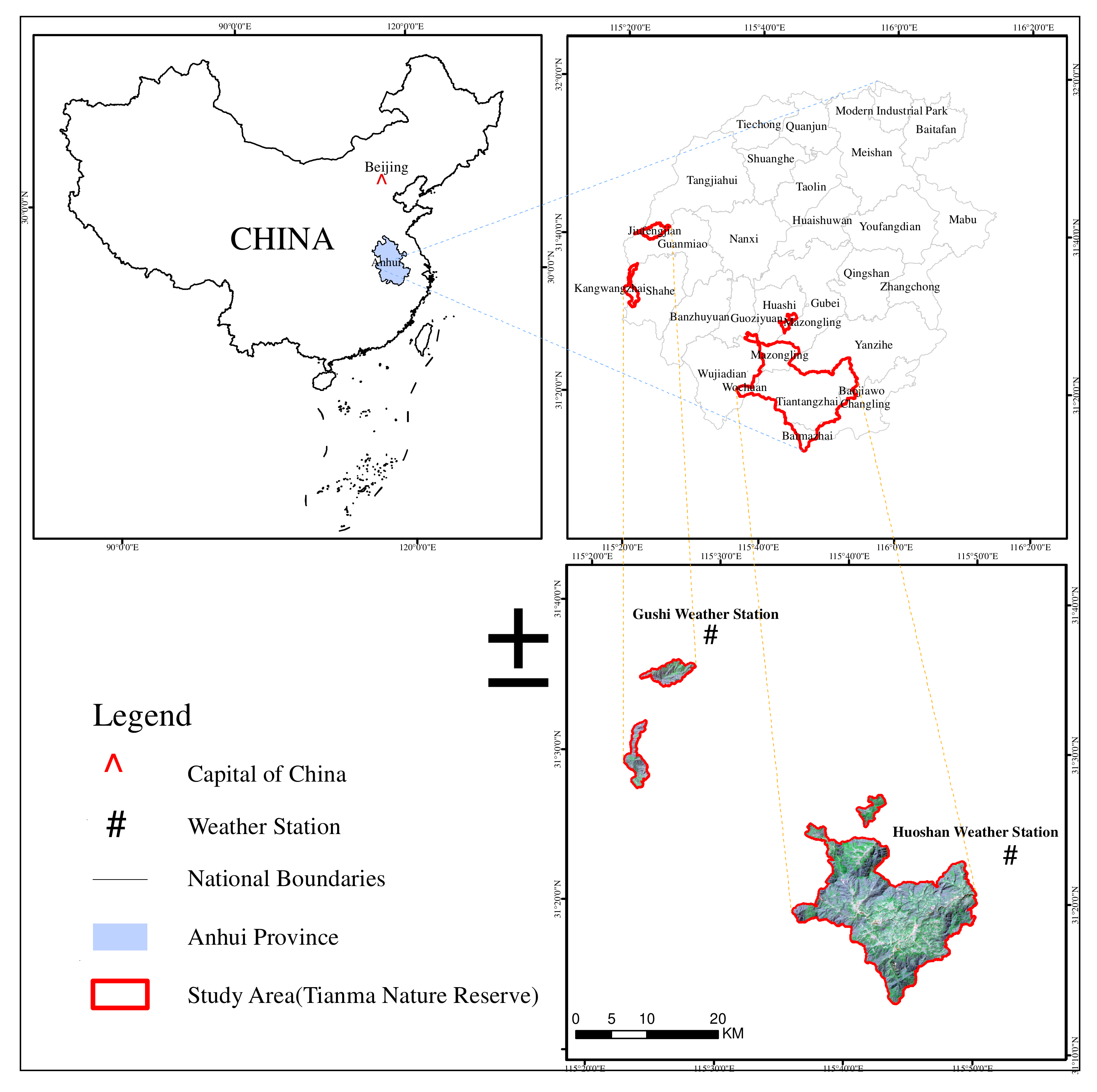
2.1. Overview of the Study Area

Tianma National Nature Reserve is in Jinzhai County, Anhui Province (31°10′–31°20′N, 115°20′–115°50′E), and it is in the hinterland of Dabie Mountain in the ecotone of Hubei, Henan, and Anhui Provinces (Figure 1). The reserve is a transition area from the northern edge of the subtropical zone to the warm temperate zone in Eastern China. The reserve preserves a relatively complete area of natural broad-leaved forests in the north subtropical zone of China. Its vertical distribution of vegetation is clear. The conservation areas of the reserve are the north subtropical evergreen and deciduous broad-leaved forest. The broad-leaved forest in this study is the natural secondary oak deciduous broad-leaved forest. Its forest stands are mostly middle-aged forest and near-mature forest. The Regulations of the People’s Republic of China on Nature Reserves stipulates that forestry production and management activities shall not be carried out in nature reserves, forest cutting is strictly prohibited, and protection priority and natural restoration are emphasized. This reserve covers an area of 28,930 hectares, consisting of Tiantangzhai Town and Mazongling Area, Wanshadang Area, Kangwangzhai Area, and Jiufengjian Area. The reserve belongs to the northern subtropical humid monsoon climate zone, which is characterized by four distinct seasons, mild climate, varying spring temperature, abundant rainfall, significant plum rains, and concentrated summer rains. Its average annual temperature is 13.5 °C, annual rainfall is 1400–1600 mm, annual sunshine hours are 2225.5 h, and average altitude is 900 m. The area of broad-leaved forest reaches 35% of the entire reserve, and the major broad-leaved tree species include Quercus serrata Murray var. brevipetiolata (A.DC.) Nakai, Castanea seguinii Dode, Cyclobalanopsis glauca (Thunb.) Oerst., Quercus acutissima Carruth., Carya cathayensis Sarg., Emmenopterys henryi Oliv., Toona sinensis, Paulownia fortunei (seem.) Hemsl., Platycarya strobilacea Sieb. et Zucc., Celtis sinensis Pers., Liquidambar formosana Hance, and Pistacia chinensis Bunge.

2.2. Data

2.2.1. Sample Plot Data

The biomass sampling survey was conducted from 23 July to 31 July 2019. Typical sampling methods were used to establish broad-leaf forest plots of different ages and stand conditions to comprehensively investigate the forest resources in the study area. All sample plots were 20 m × 20 m, and all the living trees in the plots with a diameter at breast height more than 5 cm were measured. Differential GPS (DGPS) was used to determine the geographic locations of the sample plots. The calculation method of forest biomass, proposed by Li and Lei [45], is the most widely used method for calculating of mixed broad-leaved forest biomass. Its specific formula is
W = 0.044 ( D 2 H ) 0.9169 + 0.023 ( D 2 H ) 0.7115 + 0.0104 ( D 2 H ) 0.9994 + 0.0188 ( D 2 H ) 0.8024
where W (Mg ha−1) is the forest biomass, D (cm) is the breast diameter, and H (m) is the tree height. Finally, estimated biomass data and its location of 35 sample plots were obtained, and they were used to establish a forest biomass model by machine learning.

2.2.2. Satellite Images

WorldView-2 satellite images are used in this study for remote sensing quantitative model construction of broad-leaved forest biomass in conjunction with the abovementioned forest survey data. They were taken on 23 June 2019, with a spatial resolution of 0.46 m panchromatic image and 1.85 m multispectral image, and they were used to determine the key input variables of machine learning model derived from satellite data. The remote sensing data used to retrieve the temporal and spatial distribution of forest biomass are ten scenes of Landsat series satellite image from 1998 to 2016 (http://www.gscloud.cn/ accessed on 1 March 2021), whose detailed image parameters are shown in Table A1. The time interval of two adjacent images is about 2 years, ensuring that the cloud amount of each image in the study area is less than 1% to meet the requirements of further data analysis. Radiation correction of remote sensing data was performed using ENVI5.3 to obtain irradiance data, and the FLAASH module of MODTRAN4+ radiative transfer model was used to perform atmospheric correction of irradiance data to obtain remote sensing reflectance images.

2.2.3. Meteorological Data

The meteorological data used in this study are from a weather database for the public (http://data.sheshiyuanyi.com/WeatherData/ accessed on 5 March 2021), and its dataset is the record of China’s general ground meteorological observatory, including temperature, precipitation, humidity, sunshine duration, ground temperature, and evaporation. Considering that there is no weather station inside the study area, it is impossible to obtain its local meteorological data directly. Therefore, this study uses the data of two nearby weather stations (Huoshan station and Gushi station, Figure 1). Most of the data come from Huoshan station. However, there are missing records for limited time at Huoshan station, so those records from Gushi station are used in 2015. All weather data records include 44 statistical factors such as monthly maximum temperature, monthly minimum temperature, monthly precipitation, and solar radiation (Table 1). After postprocessing these weather data, the meteorological factors of 24 months before the imaging time of each Landsat image are used for further analysis and to model forest biomass change.

2.3. Remote Sensing Classification of Forest Types

After remote sensing image preprocessing, ENVI5.3 software was used to monitor and classify the ten images from 1998 to 2016. The land use types of Tianma Nature Reserve were categorized into four forest types: broad-leaved forest, coniferous forest, coniferous and broad-leaved mixed forest, and nonforest land. Random forest method, maximum likelihood method, and Marxist distance method were selected to classify forest types. Kappa coefficient (i.e., an index to measure the accuracy of classification) and validation data were used to test the accuracy [15,46]. After classification, majority/minority processing was carried out to obtain the remote sensing classification results of forest types in the reserve.

2.4. Selection of Biomass Remote Sensing Estimation Factors

In order to obtain as many comprehensive remote sensing factors related to forest biomass as possible, this study initially screened 36 candidate factors from vegetation index, topography factor, and texture factor. These factors are B532_contrast, B532_correlation, B532_dissimilarity, B532_entropy, B532_homogeneity, B532_mean, B532_secondary moment, B532_variance, B3_contrast, B3_dissimilarity, B3_entropy, B3_homogeneity, B3_mean, B3_secondary moment, B3_variance, B4_dissimilarity, B4_entropy, B4_homogeneity, B4_mean, B4_secondary moment, B4_variance, B5_contrast, B5_correlation, B5_dissimilarity, B5_entropy, B5_homogeneity, B5_mean, B5_secondary moment, B5_variance, Slope, DVI, EVI, MSAVI, RVI, SAVI, and NDVI. The descriptions of these factors are shown in Table 2. B532 refers to the combination of Landsat band 5, 3, and 2. B3, B4, and B5 refer to bands 3, 4, and 5, respectively. Vegetation index and texture information are obtained by using corresponding band information in ENVI5.3, and slope factor is extracted from 30-m DEM data in ArcGIS10.2.

2.5. Identify Core Factors from Candidates

In general, there is redundant information among the above 36 possibly related factors, because some of them are derived from the same sources (e.g., NIR1, Red). It is necessary to identify some core factors as the inputs to machine learning models, so that computation loads can be reduced, and important features can be extracted easily.
The idea to identify the core factors is to try to eliminate some factors which have high correlation with other factors. Instead of using Pearson correlation coefficient, which can only measure linear relationship, nonlinear correlation coefficient (NCC) [47] was used to estimate the relationship between two factors.
Given 1005 random selected samples of the 36 factors from the same noncloudy WorldView-2 scene of the reserve on 23 June 2019, NCCs were estimated between any two factors among those 36 factors. After removing the factors with high NCC (i.e., NCC > 0.6), 19 remaining factors were selected as the core factors with no or low correlation to each other. These 19 core factors are list in Table 3, and they are used as input variables of the machines learning models in this study.

2.6. Machine Learning Algorithm

In this study, three machine learning algorithms of random forests (RF), support vector machine (SVM), and artificial neural network (ANN) are selected as candidates to construct a suitable forest biomass retrieve model.

2.6.1. RF

The RF algorithm is a machine learning algorithm proposed by Breiman [48]. Firstly, bootstrap samples are used to extract K samples with the same sample size from the original training set. Then, a decision tree model is established for each sample to obtain K classification results. Finally, each record is voted on according to the K classification results to determine its final classification [48]. This algorithm is the extension of the traditional decision tree algorithm by combining multiple decision trees to improve prediction accuracy [49].
In the regression analysis of biomass estimation by RF, there are two key parameters: ntree and mtry. Ntree is the number of decision trees that are resampled using bootstrap. Mtry is the number of random features, i.e., the number of input variables, whose size is usually one third of the number of input variables. However, mtry needs to be optimized to achieve an optimal model [50].

2.6.2. SVM

SVM is a supervised learning algorithm. In forest applications, it was mainly used for forest classification and then developed into the inversion and regression of forest biomass. For SVM, data are points in an N-dimensional space, and the purpose is to find the best N-1 hyperplanes to segment the points in the N-dimensional space. The key problems of SVM are kernel function selection and parameter combination optimization. The commonly used kernel functions are linear kernel function, polynomial kernel function, and Gaussian kernel function. The advantage of SVM is that it is supported by mathematical theory and has strong interpretability. For a given training sample D = {( x 1 , y 1 ) , ( x 2 , y 2 ), …… ( x i , y i ) …… ( x n , y n )}, generally, linear regression models attempt to obtain a prediction function f(x) by learning to minimize the sum of squared errors (SSE) between the observed and predicted values of dependent variable. However, one drawback of minimizing SSE is that the parameter estimation of the model will be affected by some points far away from the overall trend of the data. To avoid this issue, SVM is implemented by assuming that the model can tolerate deviations of at most ε (ε > 0) between the observed and predicted. Those points with absolute values of residuals less than ε will not contribute to the SVM, while those with greater than ε will contribute to the model in a linear proportion, such that large outliers will only have a limited effect on SVM, as there is no squared residual involved [51,52].

2.6.3. ANN

ANN started in the 1940s and is one of the earliest machine learning methods, working by imitating human brain neural network to process and memorize information [53]. ANN is a multilayer feedforward neural network with forward propagation of information and backward propagation of error. Information is first processed layer by layer from input layer through hidden ones. Output results in output layer are compared with the expected values. When the error between the output results and the expected values is greater than a predetermined value, backward propagation is performed. Then, network weights and thresholds are adjusted by the prediction error, and the network is transferred back to the forward propagation. This process is repeated until the error is less than the predetermined value, so that the output values and the predicted ones are close enough [54,55].

2.7. Construction of Remote Sensing Quantitative Model of Broad-Leaved Forest Biomass and Model Accuracy Assessment

Using the 35 samples (from Section 2.2.1) with their corresponding 19 core factors (from Section 2.5), three machine models (i.e., RF, SVM, and ANN) were trained to compare their performances, so that the best one can be selected as the best prediction model in this study. All data (including factors and biomass) were rescaled onto [–1,1], so that they are all dimensionless variables at the same scale. Then, 70%/15%/15% (i.e., 25/5/5) samples were randomly selected as the training/testing/validation samples. Because the number of 35 samples is not a large amount, it is not a wise way to use many hidden layers and hidden nodes in ANN. Fifteen hidden nodes and up to three hidden layers were used to identify the best ANN structure in this study. After comparison, three hidden layers with 8 × 5 × 2 nodes were chosen as the best ANN structure.
Cross validation is a method that can be used to estimate the performance of machine learning algorithms, and its variance is smaller than the segmentation variance of a single training test set. In this study, determination coefficient (R2) and root mean square error (RMSE) are used to evaluate the accuracy.
R 2 = i = 1 N ( x i x ¯ ) y i y ¯ 2 i = 1 N ( x i x ¯ ) 2 i = 1 N ( y i y ¯ ) 2
R M S E = 1 N i = 1 N ( y i x i ) 2
where x i   is the ith observed value, y i is the ith model estimated value, N is the size of x and y, x ¯ is the average value of x, and y ¯ is the average value of y.

2.8. Analysis on Broad-Leaved Forest Biomass Dynamic Change Driving Forces

In order to identify the major driving factors of biomass change in terms of climate, the 44 climate factors in Table 1 were used to estimate their Pearson correlation coefficients with the mean biomass change (BC), which is the difference of mean biomass (MB) of the entire reserve over two adjacent observational times (i.e., about two years). In particular, BCi = MBi – MBi−1. We can determine some driving forces of broad-leaved forest biomass dynamic change based on p values.

3. Results and Analysis

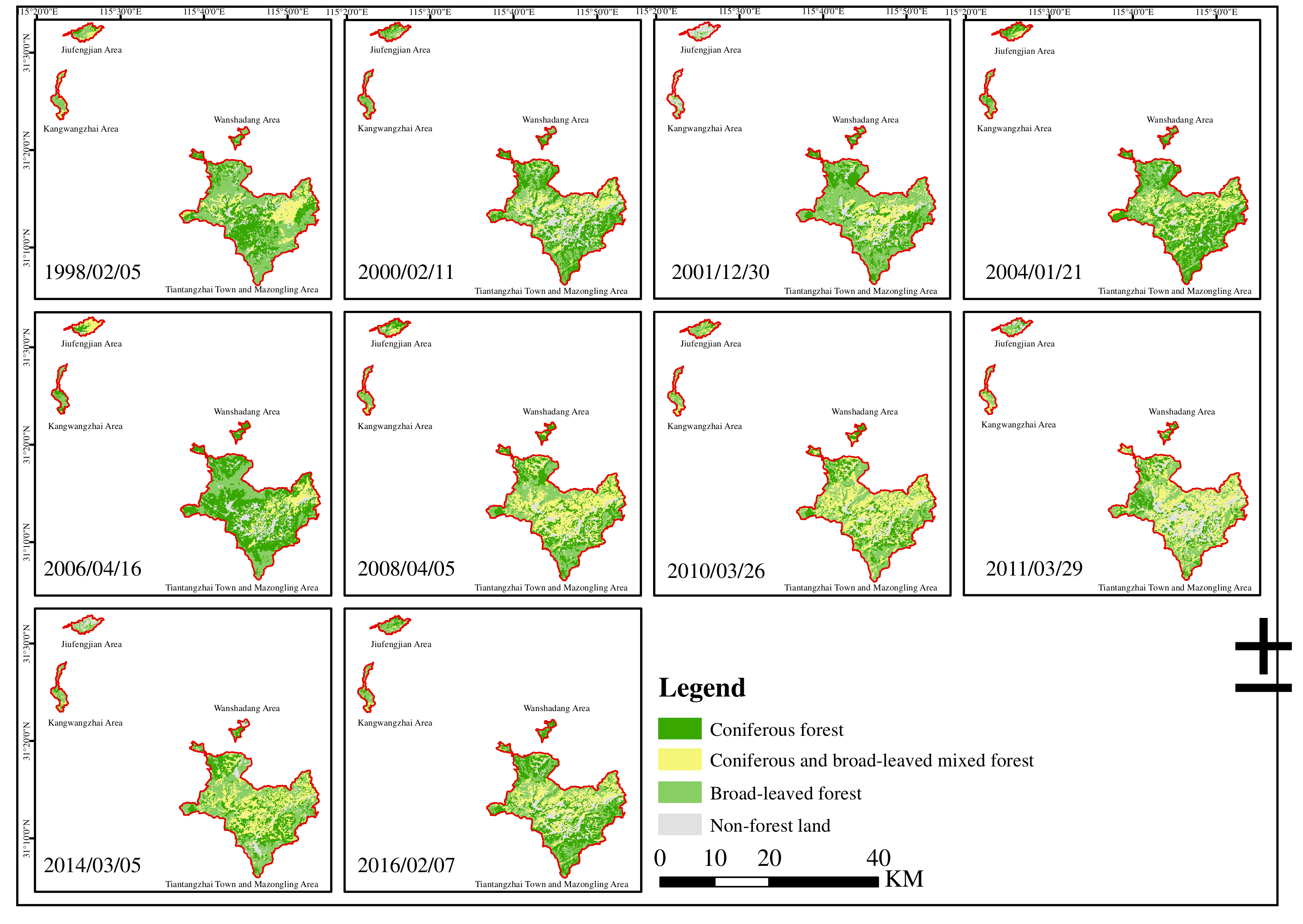
3.1. Remote Sensing Classification Results of Forest Types in Tianma National Nature Reserve

The Kappa coefficients for remote sensing classification of forest types in random forest method, maximum likelihood method, and Marxist distance method were 0.97, 0.92, and 0.80, respectively. Therefore, the random forest method with the greatest Kappa coefficient was chosen to classify the remote sensing images of the study area in this study, and its classification results are shown in Figure 2.

3.2. Construction of Remote Sensing Quantitative Model of Broad-Leaved Forest Biomass

The results of the three models (RF, SVM, and ANN) are list in Table 4, which indicates that ANN has the best performance, with high R2 and low RMSE. Thus, ANN with 8 × 5 × 2 structure was chosen as the best machine learning model to retrieve broad-leaved forest biomass in this study. Please note that both SVM and ANN models were from the Statistics and Machine Learning Toolbox of Matlab R2019b, and RF model was from “randomForest” package of R language.

3.3. Spatial Distribution of Broad-Leaved Forest Biomass in the Reserve

After applying the ANN model to 19 core factors (from Section 2.5) derived from the ten Landsat images from 1998 to 2016, the biomass data of effective pixels of broad-leaved forest were obtained in Tiantangzhai Town and Mazongling area, Wanshadang area, Kangwangzhai area, and Jiufengjian area. The numbers of effective pixels of each image are shown in Table A2. Because the position and number of effective pixels in each image are different, only the averaged biomass within a region can be analyzed meaningfully. Therefore, the mean biomasses of each area and the entire nature reserve were calculated, and results are shown in Figure 3.
As a result, the mean biomass of the broad-leaved forest in the entire nature reserve was between 90–145 Mg ha−1 from 1998 to 2016, and the temporal change characteristic was clear. It showed a change characteristic of “decreasing–increasing–decreasing–increasing–decreasing”, and it reached the lowest value of only 92.9 Mg ha−1 in 2006. The characteristic of mean biomass change in each area is consistent with the entire nature reserve. From the results, it is not clear what causes the time variation of biomass, thus it will be studied in the next section.
In addition, the results of the spatial dynamic distribution of broad-leaved forest biomass in each area and the entire reserve are shown in Figure 4.

3.4. Analysis on Broad-Leaved Forest Biomass Dynamic Change Driving Forces in the Reserve

Based on P values, only four significant climate factors (p < 0.05) were identified (Table 5); besides, the correlation between BC and its previous MB (PMB) was also calculated (i.e., the correlation between BCi and MBi−1), and its result shows that it is also a significant factor (Table 5).
Based on the four significant identified climate factors in Table 5, a regression model of biomass change was constructed. However, very high correlation was noticed between total daily maximum surface temperature (TmaxT) and average daily maximum surface temperature (Tmax) (CC = 0.9998, P = 1.87 × 10⁻¹³), so TmaxT can be removed from the modeling. The linear regression model based on climate factors becomes
BC = 282.8201 + 7.2221 × T max   0.2269 × P max +   2.9199 × Tavg
where Pmax is max precipitation, Tavg is max mean temperature, regression’s corresponding R2 = 0.8063, CC = 0.8979 (P = 0.001). After the coefficients of Tmax, Pmax, and Tavg are transformed into standardized coefficients, their corresponding standardized coefficients are 0.5177, –0.5384, and 0.0799, respectively. It indicates that, when only climate factors are considered in modeling BC, Tavg is less important, while Tmax and Pmax are equally important. Considering that the mean biomass of the previous time (i.e., PMB) was significantly related to BC (see Table 5), PMB is then added as an additional variable to the above regression. The updated linear regression model then becomes
BC = 31.6973 + 5.1720 × T max   0.2225 × P max   0.8564 × T avg 0.5260 × P MB
This updated regression is with R2 = 0.8873, CC = 0.9420 (P = 1.4656 × 10⁻⁴). This updated regression is more accurate than the previous one, implying that PMB plays a very import role in modeling BC. After transforming the coefficients of Tmax, Pmax, Tavg, and PMB into standardized coefficients, their standardized coefficients are 0.3707, −0.5279, –0.0234, and –0.3727, respectively. It implies that Tavg is still relatively insignificant, but Tmax, Pmax, and PMB are significant, although Pmax and PMB have negative impact on BC.
In addition, it is noticeable that the negative correlation between mean BC and maximum precipitation becomes more significant as the study area is closer to the climate observatory, which is shown in Figure 5. It implies that higher negative correlation could be observed if more accurate precipitation observations can be provided in the study area.

4. Discussion

Forests cover about one third of the land surface; there are many studies on forest aboveground biomass, and most of them have focused on tropical and subtropical regions [56]. This study area is located in the transition region from the northern edge of the subtropical zone to the warm temperate zone. Its results can provide not only evidence for the response of climate factors to forest biomass changes in a single-temperature zone, but also a basis for further research on the response mechanism of climate factors to forest biomass changes in different temperature zones. At large scales, how to accurately predict forest biomass and explore the dominant factors of forest biomass changes in spatiotemporal space is always a hot topic and difficult problem in forest ecology research [46]. In addition to climate factors, forest age, human disturbance, forest management activities, and other factors can affect, more or less, the change of forest biomass in previous studies [34,57,58,59,60]. These factors are easy to analyze for even-aged forests with complete data storage and small time gradient. However, for the Tianma Nature Reserve, broad-leaved forest is its secondary major natural forest. With the natural growth and renewal of trees, forest age is hard to accurately know. In-depth analysis of the dominant factors of forest biomass changes in spatial and temporal scales could be started by integrating forest parameters, climate factors, land use, management activities, and other factors. In this study, we compared three machine learning algorithms (i.e., RF, SVM, ANN), constructing the biomass estimation model of broad-leaved forest by using ground survey data and high-resolution remote sensing images. The accuracy of the model reaches R2 = 0.8742, which is much higher than that of the traditional linear or nonlinear model [61]. Compared with other areas in China, for example, Wu et al. obtained the inversion results of forest aboveground biomass (R2 = 0.9, RMSE = 16.9 Mg ha−1) by using random forest algorithm [62]. Li et al. built a broad-leaved forest biomass estimation model based on XGBoost machine learning algorithm with R2 = 0.8, RMSE = 19.25 Mg ha−1 [63]. Luo et al. constructed a broad-leaved forest biomass estimation model with model accuracy R2 = 0.73 and RMSE = 24.67 Mg ha−1, respectively [64]. Compared with other regions in the world, the optimal model R2 constructed by some researchers in Congo was 0.86, and RMSE was 10.22 Mg ha−1 [65]. Pablito et al. used SVM algorithm to obtain the estimation model of forest biomass in northwestern Mexico, with an accuracy of R2 = 0.8 [66]. In general, the model accuracy obtained in this study is on the same level as previous and latest models. By randomly selecting more than 1000 broad-leaved forest pixel points in the study area to screen remote sensing modeling factors, its data volume for training is larger than that of the traditional ground survey. This provides a new method for remote sensing estimation of forest biomass in the areas lacking ground survey data in some historical satellite images. This study starts from the establishment year of Tianma National Nature Reserve, with a timespan of about 20 years. It uses about two years as time interval, which is finer than a span of 5 years or 10 years in current literature, so that it can detect the details of forest biomass changes on a smaller timescale.
On the other hand, previous literature mostly focused on the construction of biomass model. This study aims to find the variation of biomass changes more accurately, so biomass change instead of biomass is modeled directly. The model results showed that the regressions correspond with R2 = 0.8063 and CC = 0.8979 (P = 0.001). Considering that the mean biomass of the previous time (i.e., PMB) was significantly related to BC, PMB is added as an additional variable to improve the above regression. The resulting updated linear regression model showed better results, with R2 = 0.8873 and CC = 0.9420 (P = 1.4656 × 10⁻⁴).
Our results imply that temperature has significantly positive correlation with forest biomass, which is consistent with most studies [67,68]. When the precipitation is sufficient or excessive in the growing season, the absorption and accumulation of aerobic minerals in the tree root will be reduced. Additionally, the precipitation is significantly negatively correlated with the radial growth of trees [69,70]. It was noted that when the average annual precipitation is greater than 900 mm, tree growth decreases with increasing annual precipitation [71]. The annual precipitation of Tianma Nature Reserve is 1400–1600 mm, and the rainfall is abundant. Such annual precipitation has negative correlation with forest growth, thereby affecting the reduction of forest biomass in the reserve. It can also confirm the conclusion in this study that the maximum precipitation is negatively correlated with the variation of biomass in the model.
In China, the north subtropical region mainly includes Anhui, Jiangsu, Zhejiang, Hubei, Jiangxi, Hunan, and the southern part of Henan Province. In the study of comparing the estimation model algorithms of aboveground forest biomass in subtropical China, researchers took Zhejiang Province as the research area, and the biomass predicted by ANN model was from 19.1 to 187.1 Mg ha−1, and the average biomass was 88.4 Mg ha−1 [72]. In the process of taking the forest biomass of Yushan National Forest Park in Jiangsu Province as the research object, the aboveground biomass data of the broad-leaved forest sample plot investigated ranged from 32.03 Mg ha−1 to 219.67 Mg ha−1, and the average biomass was 96.76 Mg ha−1. The minimum value predicted by the model was 8.79 Mg ha−1 and the maximum was 206.79 Mg ha−1 [73]. In the northwest of Hunan province, the minimum and maximum aboveground biomass of the surveyed broad-leaved forest plots were 9.42 Mg ha−1 and 223.35 Mg ha−1, respectively. The predicted biomass was mostly <30 or >150 Mg ha−1 [74]. Xiangjiang River is located in the subtropical monsoon humid climate zone, and the entire basin passes through Hunan and Jiangxi Province. Their results showed that the aboveground biomass of broadleaf forest predicted ranged from 4.93 to 189.30 Mg ha−1 [75]. Therefore, our results that predicted biomass of broad-leaved forest biomass ranged from <60 to >160 Mg ha−1 are reasonable. At present, the broad-leaved forest in this study is still in the early and middle stages of natural succession and has not reached the stage of zonal top community. Due to the lack of necessary forest management measures, the growth of natural secondary broad-leaved forest in mountainous areas is relatively slow. However, the biomass per unit area of tree layer would increase with the increase of age and growth of stand, and the AGB per unit area will also increase with the increase of age and growth of stand with the succession progress.

5. Conclusions

In this study, we applied the forest ground survey data of 2019 to calculated surveyed AGB for broad-leaved forest following the study from Li and Lei [46]. As high-resolution remote sensing images could reflect the position of ground objects and predicted biomass accurately, we extracted 36 candidate factors from WorldView-2 satellite images of 2019 and DEM, and 19 factors were selected as the core factors with no or low correlation to each other. By comparing three machine learning algorithms (i.e., RF, SVM, and ANN), ANN was identified as the best method of remote sensing biomass model for broad-leaved forest with R2 = 0.8742 and RMSE = 0.1531. This method was further carried out to estimate broad-leaved forest biomass from 1998 to 2016 using ten Landsat series historical remote sensing images. The results showed that the mean biomass of broad-leaved forest in the reserve was between 90–145 (Mg ha−1) from 1998 to 2016.
It is known that biomass is a cumulative value at a specific time. In order to reflect the driving factors of biomass change more scientifically and accurately, BC with two-year resolution was introduced as the dependent variable. Four significant climate factors (i.e., TmaxT, Tmax, Pmax, and Tavg) were identified from 44 candidate factors through regression analysis. A linear regression model excluding TmaxT was constructed because of the very high correlation between TmaxT and Tmax. Furthermore, the linear regression model was with higher accuracy (R2 = 0.8873, CC = 0.9420 (P = 1.4656 × 10⁻⁴)) when PMB was introduced. It implied that Tavg was relatively insignificant, but Tmax, Pmax, and PMB were significant, although Pmax and PMB had negative impact on BC.
Those approaches in this study are useful for improving the national estimation of carbon storage within aboveground biomass of broad-leaved forest and will improve the capacity to report carbon storage at Tianma National Nature Reserve, forest areas of the same forest type, and elsewhere. The research results can provide reference for other forest types. More importantly, our approaches and results can be used to evaluate the proportion and role in subtropics for forest ecosystem.

Author Contributions

Conceptualization, Z.S., Q.H. and X.T.; Formal analysis, Z.S., X.T., Q.H. and D.Y.; Funding acquisition, X.T. and Q.H.; Methodology, Z.S., X.T. and Q.H.; Investigation, X.T., Q.O. and D.Y.; Software, W.Q., H.L. (Haomiao Lu), H.L. (Hayian Lv) and Q.O.; Supervision, Z.S. and X.T.; Writing—original draft preparation, H.L. (Hayian Lv) and W.Q.; Writing—review and editing, Z.S. and X.T. All authors have read and agreed to the published version of the manuscript.

Funding

This research was funded by Anhui Provincial Natural Science Foundation (Grant NO.1808085QC74), Anhui Dabie Mountains Forest Ecosystem Research Station (Grant NO.2020132041), and Key Project of Natural Science Foundation of Anhui Education Department (Grant NO.KJ2019A0218).

Acknowledgments

The authors are thankful to Meiqin Xie, Peng Fan, Jun Ye, and Genshen Fu for surveying and data processing in the study.

Conflicts of Interest

The authors declare no conflict of interest.

Appendix A

Table A1. Information of remote sensing images in study area from 1998 to 2016.
Landsat Image IDImaging DateSensor TypeCode NumberLine NumberData LevelSpatial Resolution
LT51220381998036BJC005 February 1998TM12238L1T30
LT51220382000042BJC0011 February 2000TM12238L1T30
LT51220382001364BJC0030 December 2001TM12238L1T30
LT51220382004021BJC0021 January 2004TM12238L1T30
LT51220382006106BJC0216 April 2006TM12238L1T30
LT51220382008096BJC015 April 2008TM12238L1T30
LT51220382010085BKT0026 March 2010TM12238L1T30
LT51220382011088BJC0029 March 2011TM12238L1T30
LC81220382014064LGN015 March 2014ETM+12238L1T15
LC81220382016038LGN007 February 2016ETM+12238L1T15
Table A2. Counts of valid pixels for different scenes in four different regions of the reserve.
Date of SceneRegion 1Region 2Region 3Region 4
5 February 199889,155307677894753
11 February 200060,929200589295487
30 December 2001125,408138845683179
21 January 200462,4066316057452
16 April 200662,4186316057452
5 April 200877,35158277732239
26 March 201082,95552271395484
29 March 201171,15649165825504
5 March 201493,16254570936271
7 February 201667,801127374526632

References

  1. Mário, J.M.; Loureiro, P.; Sachsida, A. The Dynamics of Land-use in Brazilian Amazon. Ecol. Econ. 2012, 84, 23–36. [Google Scholar] [CrossRef]
  2. Rodríguez-Veiga, P.; Quegan, S.; Carreiras, J.; Persson, H.J.; Fransson, J.E.S.; Hoscilo, A.; Ziółkowski, D.; Stereńczak, K.; Lohberger, S.; Stängel, M. Forest Biomass Retrieval Approaches from Earth Observation in Different Biomes. Int. J. Appl. Earth Obs. 2019, 77, 53–68. [Google Scholar] [CrossRef]
  3. Dixon, R.K.; Solomon, A.M.; Brown, S.; Houghton, R.A.; Trexier, M.C.; Wisniewski, J. Carbon Pools and Flux of Global Forest Ecosystems. Science 1994, 263, 185–190. [Google Scholar] [CrossRef]
  4. Canadell, J.G.; Quere, C.L.; Raupach, M.R.; Field, C.B.; Buitenhuis, E.T.; Ciais, P.; Conway, T.J.; Gillett, N.P.; Houghton, R.A.; Marland, G. Contributions to Accelerating Atmospheric CO2 Growth from Economic Activity, Carbon Intensity, and Efficiency of Natural Sinks. Proc. Natl. Acad. Sci. USA 2007, 104, 18866–18870. [Google Scholar] [CrossRef] [PubMed] [Green Version]
  5. Stegen, J.C.; Swenson, N.G.; Enquist, B.J.; White, E.P.; Phillips, O.L.; Jørgensen, P.M.; Weiser, M.D.; Monteagudo, M.A.; Nez, V.P. Variation in Above-Ground Forest Biomass across Broad Climatic Gradients. Glob. Ecol. Biogeogr. 2011, 20, 744–754. [Google Scholar] [CrossRef]
  6. Fan, W.Y.; Li, M.Z.; Yang, J.M. Forest Biomass Estimation Models of Remote Sensing in Changbai Mountain Forests. Sci. Silva. Sin. 2011, 47, 16–20. [Google Scholar] [CrossRef]
  7. Liu, L.B.; Zhou, Y.C.; Cheng, A.Y.; Wang, S.J.; Ni, J. Aboveground Biomass Estimate of a Karst Forest in Central Guizhou Province, Southwestern China Based on Direct Harvest Method. Acta. Ecol. Sin. 2020, 40, 4455–4461. [Google Scholar]
  8. Xie, T.T.; Li, G.; Zhou, G.Y.; Wu, Z.M.; Zhao, H.B.; Qiu, Z.J.; Liang, R.Y. Aboveground Biomass of Natural Castanopsis Carlesii-Schima Superba Community in Xiaokeng of Nanling Mountains, South China. Chin. J. Appl. Ecol. 2013, 24, 2399–2407. [Google Scholar] [CrossRef]
  9. Li, G.; Zhou, G.Y.; Wang, X.; Wu, Z.M.; Qiu, Z.J.; Zhao, H.B.; Liang, R.Y. Aboveground Biomass of Natural Castanopsis Fissa Community at the Xiaokeng of Nanling Mountain, Southern China. Acta. Ecol. Sin. 2011, 31, 3650–3658. [Google Scholar] [CrossRef]
  10. Jiang, Z.; Liu, D.; Chen, B.; Gao, H.; Li, G. Clonal Growth of Hippophae rhamniodes ssp. Sinensis at the Early Stage in Response to Initial Planting Density and its Regulation Mechanism of Biomass Allocation. Sci. Silva. Sin. 2017, 53, 29–39. [Google Scholar] [CrossRef]
  11. Shao, M.X.; Wen, S.Z.; He, G.X.; Zhao, X.Z.; Ouyang, Q. The Biomass Structure Characteristics of P. bournei (hemsl.) Yang Plantation in Different Ages. J. Cent. South Univ. For. Tech. 2014, 34, 44–48. [Google Scholar] [CrossRef]
  12. Shen, J.P.; Chen, D.S.; Sun, X.M.; Zhang, S.G. Modeling a Single-Tree Biomass Equation by Seemingly Unrelated Regression and Dummy Variables with Larix kaempferi. J. Zhejiang AF Univ. 2019, 36, 877–885. [Google Scholar]
  13. Wei, X.M. Estimation of Forest Aboveground Biomass Based on Multi-Source Data. Geomat. Inform. Sci. Wuhan Univ. 2019, 44, 1385–1390. [Google Scholar] [CrossRef]
  14. Esteban, J.; Mcroberts, R.E.; Fernández-Landa, A.; Tomé, J.L.; Nsset, E. Estimating Forest Volume and Biomass and Their Changes Using Random Forests and Remotely Sensed Data. Remote Sens. 2019, 11, 1944. [Google Scholar] [CrossRef] [Green Version]
  15. Pham, L.; Brabyn, L. Monitoring Mangrove Biomass Change in Vietnam Using SPOT Images and an Object-based Approach Combined with Machine Learning Algorithms. ISPRS J. Photogramm. 2017, 128, 86–97. [Google Scholar] [CrossRef]
  16. Naik, P.; Dalponte, M.; Bruzzone, L. Prediction of Forest Aboveground Biomass Using Multitemporal Multispectral Remote Sensing Data. Remote Sens. 2021, 13, 1282. [Google Scholar] [CrossRef]
  17. Nguyen, T.H.; Jones, S.; Soto-Berelov, M.; Haywood, A.; Hislop, S. Landsat Time-Series for Estimating Forest Aboveground Biomass and Its Dynamics across Space and Time: A Review. Remote Sens. 2019, 12, 98. [Google Scholar] [CrossRef] [Green Version]
  18. Lakyda, P.; Shvidenko, A.; Bilous, A.; Myroniuk, V.; Matsala, M.; Zibtsev, S.; Schepaschenko, D.; Holiaka, D.; Vasylyshyn, R.; Lakyda, I.; et al. Impact of Disturbances on the Carbon Cycle of Forest Ecosystems in Ukrainian Polissya. Forests 2019, 10, 337. [Google Scholar] [CrossRef] [Green Version]
  19. Yang, S.X.; Feng, Q.S.; Liang, T.G.; Liu, B.K.; Zhang, W.J.; Xie, H.J. Modeling Grassland Above-Ground Biomass Based on Artificial Neural Network and Remote Sensing in the Three-River Headwaters Region. Remote Sens. Environ. 2018, 204, 448–455. [Google Scholar] [CrossRef]
  20. Alimjan, G.; Sun, T.L.; Jumahun, H.; Guan, Y.; Zhou, W.T.; Sun, H.G. A Hybrid Classification Approach Based on Support Vector Machine and K-Nearest Neighbor for Remote Sensing Data. Int. J. Pattern. Recogn. 2017, 31, 1750034.1–1750034.22. [Google Scholar] [CrossRef]
  21. Liang, S.; Cheng, J.; Jia, K.; Jiang, B.; Liu, Q.; Liu, S.H.; Xiao, Z.Q.; Xie, X.; Yao, Y.; Yuan, W.; et al. Recent Progress in Land Surface Quantitative Remote Sensing. J. Remote Sens. 2016, 20, 875–898. [Google Scholar] [CrossRef]
  22. Santi, E.; Chiesi, M.; Fontanelli, G.; Lapini, A.; Paloscia, S.; Pettinato, S.; Ramat, G.; Santurri, L. Mapping Woody Volume of Mediterranean Forests by Using SAR and Machine Learning: A Case Study in Central Italy. Remote Sens. 2021, 13, 809. [Google Scholar] [CrossRef]
  23. Nandy, S.; Singh, R.; Ghosh, S.; Watham, T.; Kushwaha, S.P.S.; Kumar, A.S.; Dadhwal, V.K. Neural Network-Based Modelling for Forest Biomass Assessment. Carbon Manag. 2017, 8, 305–317. [Google Scholar] [CrossRef]
  24. Yang, J.M.; Fan, W.Y.; Li, M.Z.; Tian, L.J.; Mao, X.G.; Yu, Y. Quantitative Driving Analysis of Forest Biomass Changes in Changbai Mountain Forest Region. Chin. J. Appl. Ecol. 2011, 22, 47–52. [Google Scholar] [CrossRef]
  25. Powell, S.L.; Cohen, W.B.; Healey, S.P.; Kennedy, R.E.; Moisen, G.G.; Pierce, K.B. Quantification of Live Aboveground Forest Biomass Dynamics with Landsat Time-Series and Field Inventory Data: A Comparison of Empirical Modeling Approaches. Remote Sens. Environ. 2010, 114, 1053–1068. [Google Scholar] [CrossRef]
  26. Ghosh, S.M.; Behera, M.D. Aboveground Biomass Estimation Using Multi-Sensor Data Synergy and Machine Learning Algorithms in a Dense Tropical Forest. Appl. Geophys. 2018, 96, 29–40. [Google Scholar] [CrossRef]
  27. Raha, D.; Dar, J.A.; Pandey, P.K.; Lone, P.A.; Verma, S.; Khare, P.K.; Khan, M.L. Carbon Management Variation in Tree Biomass and Carbon Stocks in Three Tropical Dry Deciduous Forest Types of Madhya Pradesh, India. Carbon Manag. 2020, 11, 109–120. [Google Scholar] [CrossRef]
  28. Venter, M.; Dwyer, J.; Dieleman, W.; Ramachandra, A.; Gillieson, D.; Laurance, S.; Cernusak, L.; Beehler, B.; Jensen, R.; Bird, M. Optimal Climate for Large Trees at High Elevations Drives Patterns of Biomass in Remote Forests of Papua New Guinea. Glob. Change Biol. 2017, 23, 4873–4883. [Google Scholar] [CrossRef] [PubMed]
  29. Zhao, K.G.; Suarez, J.C.; Garcia, M.; Hu, T.X.; Wang, C.; Londo, A. Utility of Multitemporal Lidar for Forest and Carbon Monitoring: Tree Growth, Biomass Dynamics, And Carbon Flux. Remote Sens. Environ. 2018, 204, 883–897. [Google Scholar] [CrossRef]
  30. Wu, Z.; Dai, E.F.; Ge, Q.S.; Xi, W.M.; Wang, X.F. Modelling the Integrated Effects of Land Aboveground Biomass, Use and Climate Change Scenarios on Forest a Case Study in Taihe County of China Ecosystem. J. Geogr. Sci. 2017, 27, 205–222. [Google Scholar] [CrossRef] [Green Version]
  31. Lin, M.Z.; Ling, Q.P.; Pei, H.Q.; Song, Y.N.; Qiu, Z.X.; Wang, C.; Liu, T.D.; Gong, W.F. Remote Sensing of Tropical Rainforest Biomass Changes in Hainan Island, China from 2003 to 2018. Remote Sens. 2021, 13, 1696. [Google Scholar] [CrossRef]
  32. García-Aldés, R.; Estrada, A.; Early, R.; Lehsten, V.; Morin, X.; Dornelas, M. Climate Change Impacts on Long-Term Forest Productivity Might be Driven by Species Turnover Rather Than by Changes in Tree Growth. Glob. Ecol. Biogeogr. 2020, 29, 1360–1372. [Google Scholar] [CrossRef]
  33. Souza, A.F.; Longhi, S.J. Disturbance History Mediates Climate Change Effects on Subtropical Forest Biomass and Dynamics. Ecol. Evol. 2019, 9, 7184–7199. [Google Scholar] [CrossRef] [Green Version]
  34. Lie, G.W.; Xue, L. Biomass Allocation Patterns in Forests Growing Different Climatic Zones of China. Trees 2016, 30, 639–646. [Google Scholar] [CrossRef]
  35. Becknell, J.M.; Kissing Kucek, L.; Powers, J.S. Aboveground Biomass in Mature and Secondary Seasonally Dry Tropical Forests: A Literature Review and Global Synthesis. For. Ecol. Manag. 2020, 276, 88–95. [Google Scholar] [CrossRef]
  36. Bennett, A.C.; Penman, T.D.; Arndt, S.K.; Roxburgh, S.H.; Bennett, L.T. Climate More Important Than Soils for Predicting Forest Biomass at the Continental Scale. Ecography 2020, 43, 1692–1705. [Google Scholar] [CrossRef]
  37. Ma, W.H.; Liu, Z.L.; Wang, Z.H.; Wang, W.; Liang, C.Z.; Tang, Y.H.; He, J.S.; Fang, J.Y. Climate Change Alters Interannual Variation of Grassland Aboveground Productivity: Evidence from a 22-Year Measurement Series in the Inner Mongolian Grassland. J. Plant Res. 2010, 123, 509–517. [Google Scholar] [CrossRef]
  38. Chen, Q.; Chen, Y.H.; Wang, M.J.; Jiang, W.G.; Hou, P.; Li, Y. Change of Vegetation Net Primary Productivity in Yellow River Watersheds From 2001 to 2010 and its Climatic Driving Factors Analysis. Chin. J. Appl. 2014, 25, 2811–2818. [Google Scholar] [CrossRef]
  39. Ewe, S.; Gaiser, E.E.; Childers, D.L.; Iwaniec, D.; Rivera-Monroy, V.H.; Twilley, R.R. Spatial and Temporal Patterns of Aboveground Net Primary Productivity (anpp) along Two Freshwater-Estuarine Transects in the Florida Coastal Everglades. Hydrobiologia 2006, 569, 459–474. [Google Scholar] [CrossRef]
  40. Ortiz-Reyes, A.D.; Valdez-Lazalde, J.R.; Ángeles-Pérez, G.; De los Santos-Posadas, H.M.; Schneider, L.; Aguirre-Salado, C.A.; Peduzzi, A. Synergy of Landsat, Climate and LiDAR Data for Aboveground Biomass Mapping in Medium-Stature Tropical Forests of the Yucatan Peninsula, Mexico. Rev. Chapingo Ser. Cienc. For. Am. 2021, 27, 383–400. [Google Scholar] [CrossRef]
  41. Shen, W.J.; Li, M.S.; Huang, C.Q.; Wei, A.S. Quantifying Live Aboveground Biomass and Forest Disturbance of Mountainous Natural and Plantation Forests in Northern Guangdong, China, Based on Multi-Temporal Landsat, PALSAR and Field Plot Data. Remote Sens. 2016, 8, 595. [Google Scholar] [CrossRef] [Green Version]
  42. Pirasteh, S.; Zenner, E.K.; Mafi-Gholami, D.; Jaafari, A.; Kamari, A.N.; Liu, G.; Zhu, Q.; Li, J. Modeling Mangrove Responses to Multi-Decadal Climate Change and Anthropogenic Impacts Using a Long-Term Time Series of Satellite Imagery. Int. J. Appl. Earth Obs. Geoinf. 2021, 102, 102390. [Google Scholar] [CrossRef]
  43. Zeng, W.; Chen, X.; Yang, X. Developing National and Regional Individual Tree Biomass Models and Analyzing Impact of Climatic Factors on Biomass Estimation for Poplar Plantations in China. Trees 2020, 35, 93–102. [Google Scholar] [CrossRef]
  44. Foster, J.R.; Finley, A.O.; D’Amato, A.W.; Bradford, J.B.; Banerjee, S. Predicting Tree Biomass Growth in the Temperate–Boreal Ecotone: Is Tree Size, Age, Competition, or Climate Response Most Important? Glob. Change Biol. 2016, 22, 2138–2151. [Google Scholar] [CrossRef] [PubMed]
  45. Li, H.; Lei, Y. Estimation and Evaluation of Forest Biomass Carbon Storage in China; China Forestry: Beijing, China, 2010; ISBN 978-7-5038-5809-3. [Google Scholar]
  46. Pham, T.D.; Yokoya, N.; Bui, D.T.; Yoshino, K.; Friess, D.A. Remote Sensing Approaches for Monitoring Mangrove Species, Structure, and Biomass: Opportunities and Challenges. Remote Sens. 2019, 11, 230. [Google Scholar] [CrossRef] [Green Version]
  47. Wang, Q.; Shen, Y.; Zhang, J. A Nonlinear Correlation Measure for Multivariable Data Set. Physica D 2005, 200, 287–295. [Google Scholar] [CrossRef]
  48. Breiman, L. Random Forests. Mach. Learn. 2001, 45, 5–32. [Google Scholar] [CrossRef] [Green Version]
  49. Sheykhmousa, M.; Mahdianpari, M. Support Vector Machine Versus Random Forest for Remote Sensing Image Classification: A Meta-Analysis and Systematic Review. IEEE J. Sel. Top. Appl. Earth Obs. Remote Sens. 2020, 13, 6308–6325. [Google Scholar] [CrossRef]
  50. Júnior, I.D.S.T.; Torres, C.; Leite, H.G.; Castro, N.L.M.D.; Farias, A.A. Machine Learning: Modeling Increment in Diameter of Individual Trees on Atlantic Forest Fragments. Ecol. Indic. 2020, 117, 106685. [Google Scholar] [CrossRef]
  51. Kuhn, M.; Johnson, K. Applied Predictive Modeling; Springer: New York, NY, USA, 2013; ISBN 978-146-14-6848-6. [Google Scholar]
  52. Alimjan, G.; Sun, T.; Liang, Y.; Jumahun, H.; Guan, Y. A New Technique for Remote Sensing Image Classification Based on Combinatorial Algorithm of SVM and KNN. Int. J. Pattern. Recogn. 2018, 32, 1859012.1–1859012.23. [Google Scholar] [CrossRef]
  53. An, T.; Nandy, S.; Srinet, R.; Luong, N.V.; Kumar, A.S. Forest Aboveground Biomass Estimation Using Machine Learning Regression Algorithm in Yok Don National Park, Vietnam. Ecol. Inform. 2018, 50, 24–32. [Google Scholar] [CrossRef]
  54. Dong, L.; Du, H.; Han, N.; Li, X.; He, S. Application of Convolutional Neural Network on Lei Bamboo Above-ground-biomass (AGB) Estimation Using Worldview-2. Remote Sens. 2020, 12, 958. [Google Scholar] [CrossRef] [Green Version]
  55. Mao, H.; Meng, J.; Ji, F.; Zhang, Q.; Fang, H. Comparison of Machine Learning Regression Algorithms for Cotton Leaf Area Index Retrieval Using Sentinel-2 Spectral Bands. Appl. Sci. 2019, 9, 1459. [Google Scholar] [CrossRef] [Green Version]
  56. Gyamfi-Ampadu, E.; Gebreslasie, M. Two Decades Progress on the Application of Remote Sensing for Monitoring Tropical and Sub-Tropical Natural Forests: A Review. Forests 2021, 12, 739. [Google Scholar] [CrossRef]
  57. Dong, S.K.; Sha, W.; Su, X.K.; Zhang, Y.; Li, S.; Gao, X.X.; Liu, S.L.; Shi, J.B.; Liu, Q.R.; Hao, Y. The Impacts of Geographic, Soil and Climatic Factors on Plant Diversity, Biomass and Their Relationships of the Alpine Dry Ecosystems: Cases from the Aerjin Mountain Nature Reserve, China. Ecol. Eng. 2019, 127, 170–177. [Google Scholar] [CrossRef]
  58. De Avila, A.L.; van der Sande, M.T.; Dormann, C.F.; Pea-Claros, M.; Poorter, L.; Mazzei, L.; Ruschel, A.R.; Silva, J.M.; de Carvalho, J.O.P.; Bauhus, J. Disturbance Intensity is a Stronger Driver of Biomass Recovery than Remaining Tree-Community Attributes in a Managed Amazonian Forest. J. Appl. Ecol. 2018, 55, 1647–1657. [Google Scholar] [CrossRef] [Green Version]
  59. Chen, H.; Luo, Y.; Reich, P.B.; Searle, E.B.; Biswas, S.R.; Enquist, B. Climate Change-Associated Trends in Net Biomass Change are Age Dependent in Western Boreal Forests of Canada. Ecol. Lett. 2016, 19, 1150–1158. [Google Scholar] [CrossRef] [PubMed]
  60. Requena Suarez, D.; Rozendaal, D.M.A.; De Sy, V.; Gibbs, D.A.; Harris, N.L.; Sexton, J.O.; Feng, M.; Channan, S.; Zahabu, E.; Silayo, D.S.; et al. Variation in Aboveground Biomass in Forests and Woodlands in Tanzania along Gradients in Environmental Conditions and Human Use. Environ. Res. Lett. 2021, 16, 044014. [Google Scholar] [CrossRef]
  61. Zhao, K.; Popescu, S.; Meng, X.; Yong, P.; Ag Ca, M. Characterizing Forest Canopy Structure with Lidar Composite Metrics and Machine Learning. Remote Sens. Environ. 2011, 115, 1978–1996. [Google Scholar] [CrossRef]
  62. Wu, C.; Shen, H.; Wang, K.; Shen, A.; Deng, J.; Gan, M. Landsat Imagery-Based Above Ground Biomass Estimation and Change Investigation Related to Human Activities. Sustainability 2016, 8, 159. [Google Scholar] [CrossRef] [Green Version]
  63. Li, Y.; Li, C.; Li, M.; Liu, Z. Influence of Variable Selection and Forest Type on Forest Aboveground Biomass Estimation Using Machine Learning Algorithms. Forests 2019, 10, 1073. [Google Scholar] [CrossRef] [Green Version]
  64. Luo, M.; Wang, Y.; Xie, Y.; Zhou, L.; Qiao, J.; Qiu, S.; Sun, Y. Combination of Feature Selection and CatBoost for Prediction: The First Application to the Estimation of Aboveground Biomass. Forests 2021, 12, 216. [Google Scholar] [CrossRef]
  65. Opelele, O.M.; Yu, Y.; Fan, W.; Chen, C.; Kachaka, S.K. Biomass Estimation Based on Multilinear Regression and Machine Learning Algorithms in the Mayombe Tropical Forest, in the Democratic Republic of Congo. Appl. Ecol. Environ. Res. 2021, 19, 359–377. [Google Scholar] [CrossRef]
  66. López-Serrano, P.M.; Domínguez, J.L.C.; Corral-Rivas, J.J.; Jiménez, E.; López-Sánchez, C.A.; Vega-Nieva, D.J. Modeling of Aboveground Biomass with Landsat 8 OLI and Machine Learning in Temperate Forests. Forests 2020, 11, 11. [Google Scholar] [CrossRef] [Green Version]
  67. Zhang, Q.; Liang, Y.; He, H.; Huang, C.; Liu, B.; Jiang, S. Changes in Species-Level Biomass and Its Relationship with Climate and Forest Disturbances in the Great Xing’an Mountains. Acta Ecol. Sin. 2019, 39, 4442–4454. [Google Scholar] [CrossRef]
  68. Hisano, M.; Chen, H. Spatial Variation in Climate Modifies Effects of Functional Diversity on Biomass Dynamics in Natural Forests Across Canada. Glob. Ecol. Biogeogr. 2020, 29, 682–695. [Google Scholar] [CrossRef]
  69. Fritts, H.C.; Dean, J.S. Dendrochrological Modeling Of of the Effects of Climate Change on Tree-Ring Width Chronologies form the Chaco Canyon Area, Southwestern United States. Tree-Ring Bull. 1992, 52, 31–58. [Google Scholar]
  70. Wimmer, R.; Grabner, M. A Comparison of Tree-Ring Features in Picea Abies as Correlated with Climate. IAWA J. 2000, 21, 403–416. [Google Scholar] [CrossRef]
  71. Buechling, A.; Martin, P.H.; Canham, C.D. Climate and Competition Effects on Tree Growth in Rocky Mountain Forests. J. Ecol. 2017, 105, 1636–1647. [Google Scholar] [CrossRef] [Green Version]
  72. Gao, Y.; Lu, D.; Li, G.; Wang, G.; Chen, Q.; Liu, L.; Li, D. Comparative Analysis of Modeling Algorithms for Forest Aboveground Biomass Estimation in a Subtropical Region. Remote Sens. 2018, 10, 627. [Google Scholar] [CrossRef] [Green Version]
  73. Cao, L.; Coops, N.C.; Innes, J.; Dai, J.; She, G. Mapping Above- and Below-Ground Biomass Components in Subtropical Forests Using Small-Footprint LiDAR. Forests 2014, 5, 1356–1373. [Google Scholar] [CrossRef] [Green Version]
  74. Li, C.; Li, M.; Iizuka, K.; Liu, J.; Chen, K.; Li, Y. Effects of Forest Canopy Structure on Forest Aboveground Biomass Estimation Using Landsat Imagery. IEEE Access 2021, 9, 5285–5295. [Google Scholar] [CrossRef]
  75. Li, Y.; Li, M.; Liu, Z.; Li, C. Combining Kriging Interpolation to Improve the Accuracy of Forest Aboveground Biomass Estimation Using Remote Sensing Data. IEEE Access 2020, 8, 128124–128139. [Google Scholar] [CrossRef]
Figure 1. Location of the study area.
Remotesensing 14 01066 g001
Figure 2. Land use classifications of the Tianma Nature Reserve using random forest method from 1998 to 2016.
Remotesensing 14 01066 g002
Figure 3. Mean biomass (Mg ha−1) in Tianma Nature Reserve from 1998 to 2016 with two-year interval, including mean biomass in each area and entire reserve.
Remotesensing 14 01066 g003
Figure 4. Spatial distribution of broad-leaved forest biomass about every two years from 1998 to 2016. This study categorizes broad-leaved forest biomass into 7 classes: <60 Mg ha−1, 60–80 Mg ha−1, 80–100 Mg ha−1, 100–120 Mg ha−1, 120–140 Mg ha−1, 140–160 Mg ha−1, and >160 Mg ha−1.
Remotesensing 14 01066 g004
Figure 5. Correlation coefficient between two-year biomass change and max precipitation for each area.
Remotesensing 14 01066 g005
Table 1. All available meteorological factors in the study area. A total of 44 factors were used in this study, including temperature, precipitation, humidity, sunshine duration, and evaporation.
NumberMeteorological
Factor
NumberMeteorological
Factor
NumberMeteorological
Factor
1Total mean surface temperature (°C)16Min precipitation (mm)31Max sunshine hours (h)
2Average mean surface temperature (°C)17Total mean temperatures (°C)32Min sunshine hours (h)
3Max mean surface temperature (°C)18Average mean temperatures (°C)33Total mean relative humidity (%)
4Min mean surface temperature (°C)19Max mean temperatures (°C)34Average mean relative humidity (%)
5Total daily maximum surface temperature (°C)20Min mean temperatures (°C)35Max mean relative humidity (%)
6Average daily maximum surface temperature (°C)21Total daily maximum temperature (°C)36Min mean relative humidity (%)
7Max daily maximum surface temperature (°C)22Average daily maximum temperature (°C)37Total minimum relative humidity (%)
8Min daily maximum surface temperature (°C)23Max daily maximum temperature (°C)38Average minimum relative humidity (%)
9Total daily minimum surface temperature (°C)24Min daily maximum temperature (°C)39Max minimum relative humidity (%)
10Average daily minimum surface temperature (°C)25Total daily minimum temperature (°C)40Min minimum relative humidity (%)
11Max daily minimum surface temperature (°C)26Average daily minimum temperature (°C)41Total evaporation (mm)
12Min daily minimum surface temperature (°C)27Max daily minimum temperature (°C)42Average evaporation (mm)
13Total precipitation (mm)28Min daily minimum temperature (°C)43Average evaporation (mm)
14Average precipitation (mm)29Total sunshine hours (h)44Min evaporation (mm)
15Max precipitation (mm)30Average sunshine hours (h)
Table 2. Biomass modeling factors of broad-leaved forest in Tianma Nature Reserve. There are three types: spectral index, textural parameter, and topographic parameter.
TypeFactorDescription
Spectral indicesNDVI N I R 1 R e d / N I R 1 + R e d
RVINIR1/Red
EVI 2.5 N I R 1 R e d / ( N I R 1 + 6 N I R 1 7.5 B l u e + 1 )
DVI N I R 1 R e d
SAVI 1.5 N I R 1 R e d / N I R 1 + R e d + 0.5
MSAVI 1 2 2 N I R 1 + 1 ( 2 N I R 1 + 1 ) 2 8 ( N I R 1 R e d )
Textural ParametersEntropy i , j = 0 N 1 i P i , j l n P i , j
Secondary Moment i , j = 0 N 1 i P i j 2
Dissimilarity i , j = 0 N 1 i P i j i j
Mean i , j = 0 N 1 i P i , j
Homogeneity i , j = 0 N 1 i P i j 1 + i j 2
Correlation i , j = 0 N 1 i P i j i M E J M E V A i V A j
Contrast i , j = 0 N 1 i P i j i j 2
Variance i , j = 0 N 1 P i j i M E 2
Textural ParametersSlopeSlope (◦)
Table 3. Nineteen core factors were selected from 36 candidate factors using nonlinear correlation coefficient method.
Serial
Number
FactorSerial
Number
FactorSerial
Number
FactorSerial
Number
Factor
1B532_contrast6B532_variance11B4_dissimilarity16RVI
2B532_mean7B3_variance12Slope17B532_homogeneity
3B3_secondary moment8B5_contrast13B532_entropy18B3_mean
4B4_variance9B532_dissimilarity14B3_entropy19B4_mean
5B532_correlation10B3_contrast15B4_entropy
Table 4. Performance assessments of three different machine learning methods. R2 and RMSE were obtained through training, testing, validation, and all samples, respectively.
R2RMSE
TrainingTestingValidationAllTrainingTestingValidationAll
RF0.63340.67980.07280.66020.27790.22020.39810.2441
SVM0.86200.47050.96380.81510.17140.16430.32070.1988
ANN0.89170.87260.93040.87420.16250.12100.13190.1531
Table 5. Significant correlation (p < 0.05) between the predictive mean BC of the reserve and climate factors, as well as the PMB.
Significant FactorCCp Value
Total daily maximum surface temperature (°C)0.71690.0298
Average daily maximum surface temperature (°C)0.72060.0285
Max precipitation (mm)−0.70270.0348
Max mean temperature (°C)0.68690.0410
The mean biomass of the previous time (Mg ha1)−0.71180.0315
Publisher’s Note: MDPI stays neutral with regard to jurisdictional claims in published maps and institutional affiliations.

