
Assessment of Contemporary Antarctic GIA Models Using High-Precision GPS Time Series

 , ,
, ,
Abstract
:1. Introduction
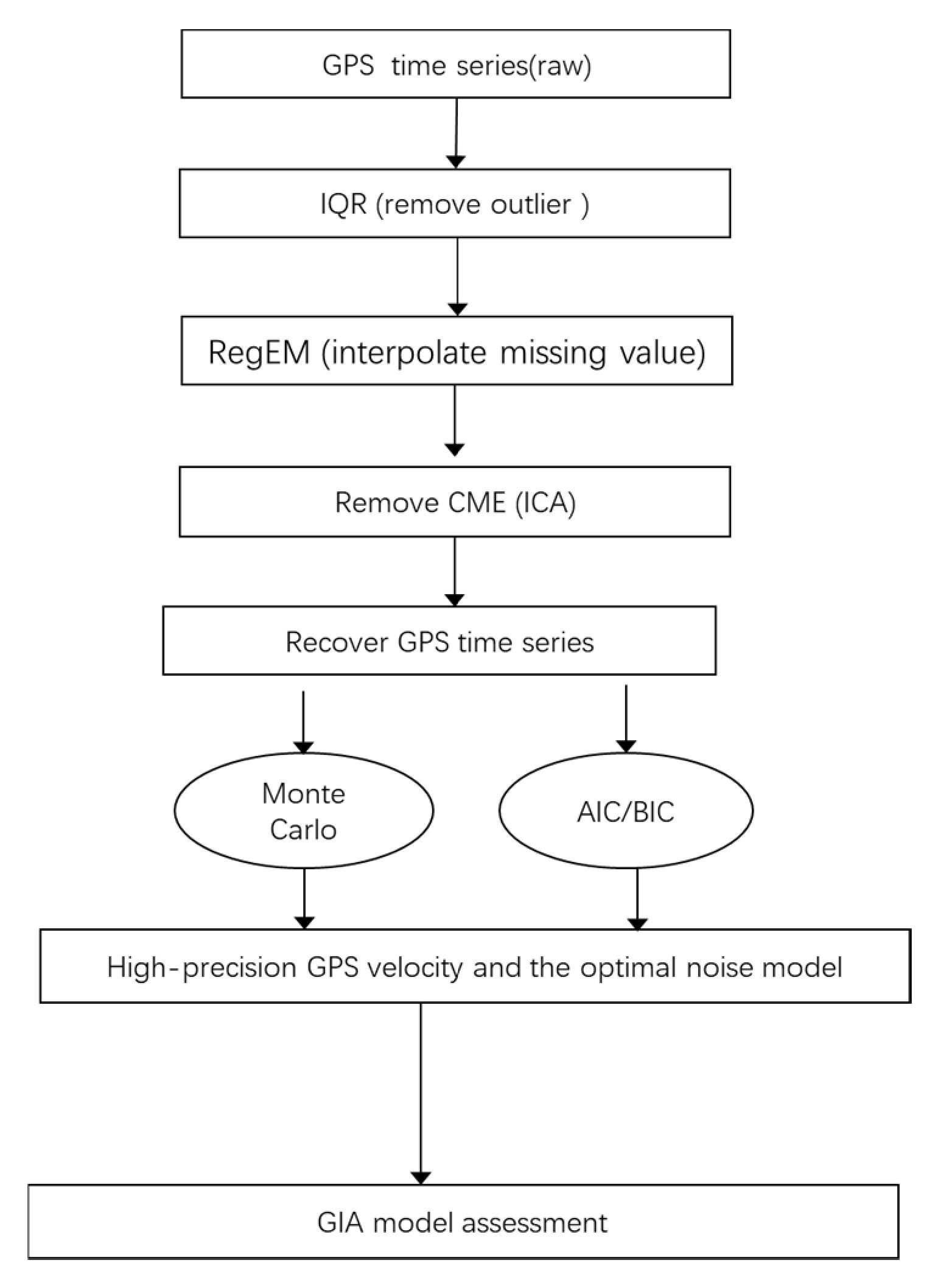
2. Materials and Methods
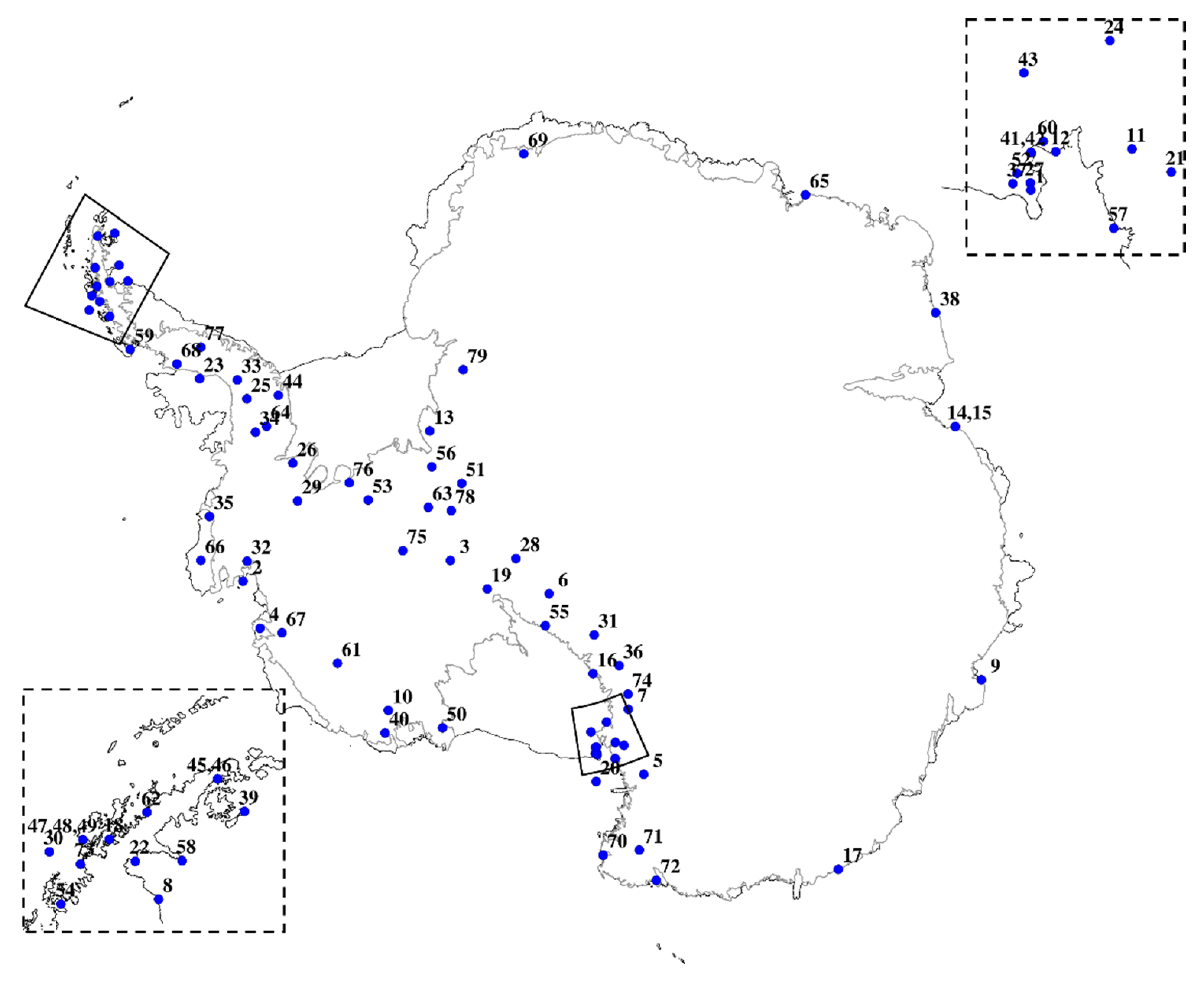
2.1. GPS Data
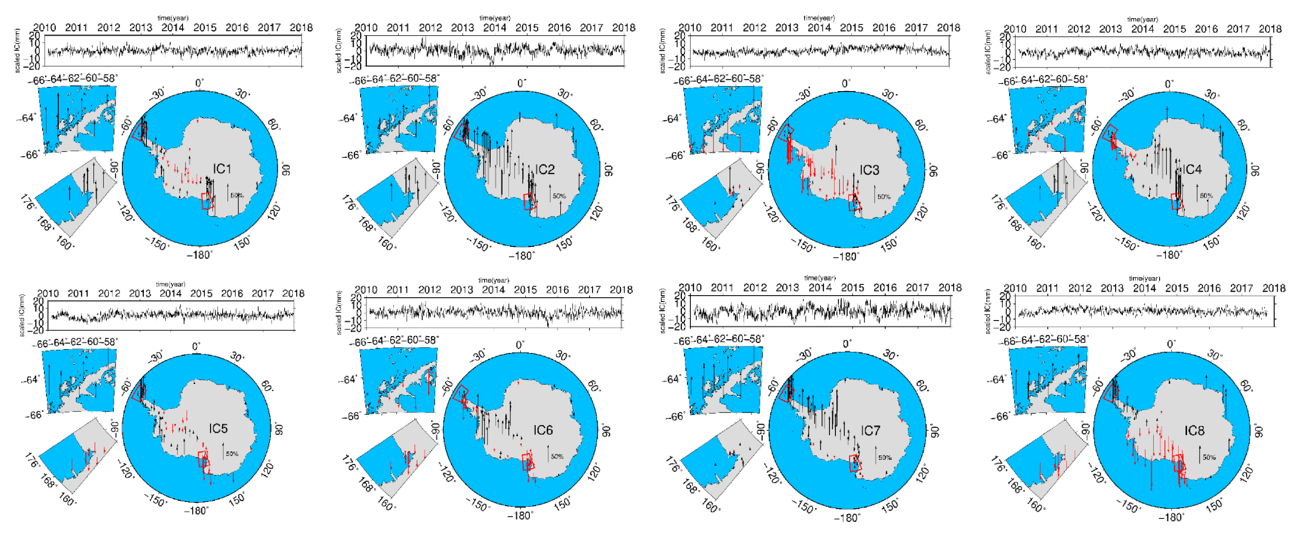
2.2. ICA Filtering
2.3. AIC and Noise Analysis
3. Results
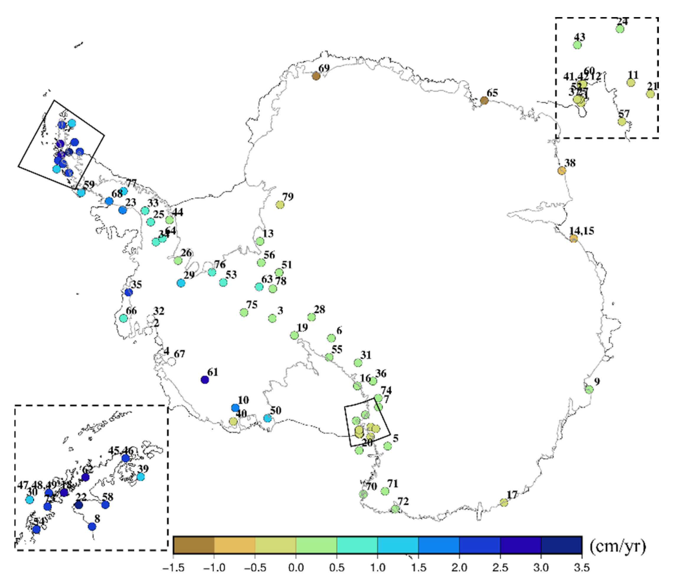
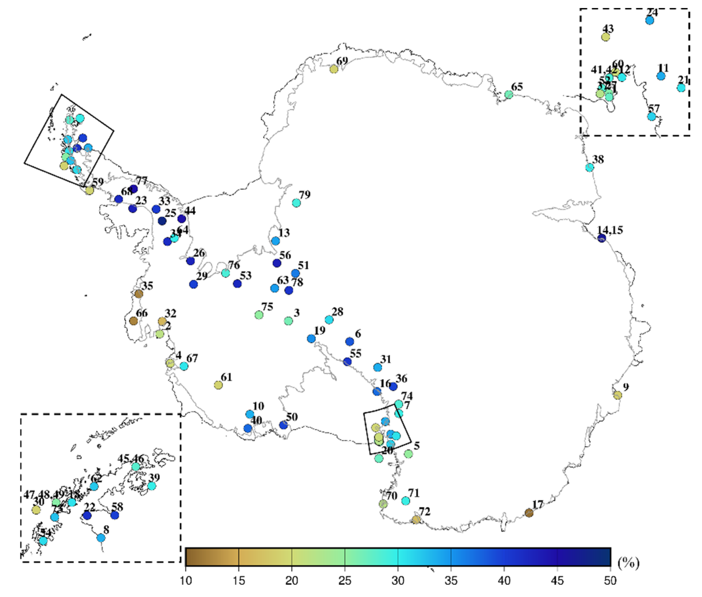
3.1. GPS Velocity Field
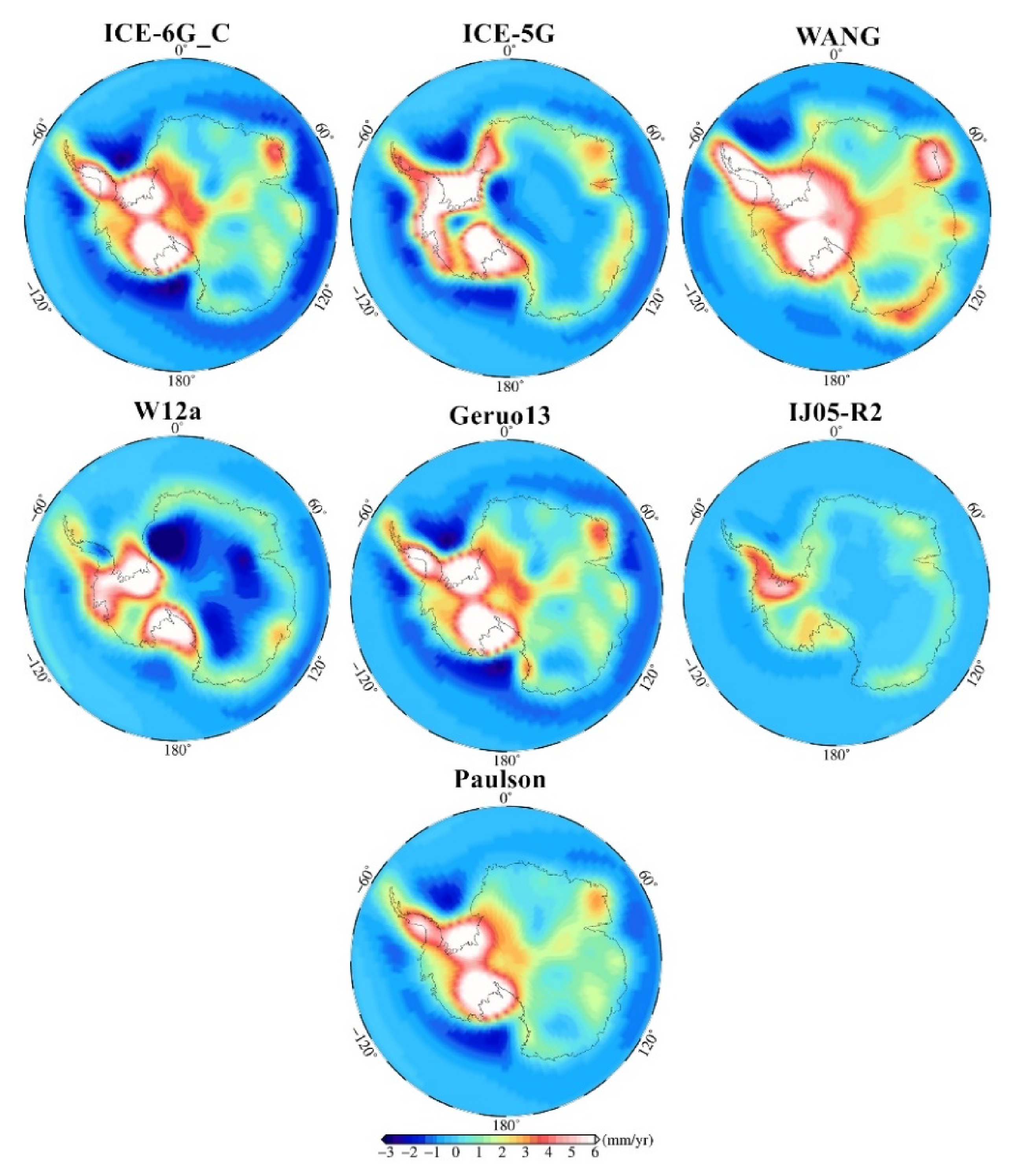
3.2. Ice Mass Elastic Loading
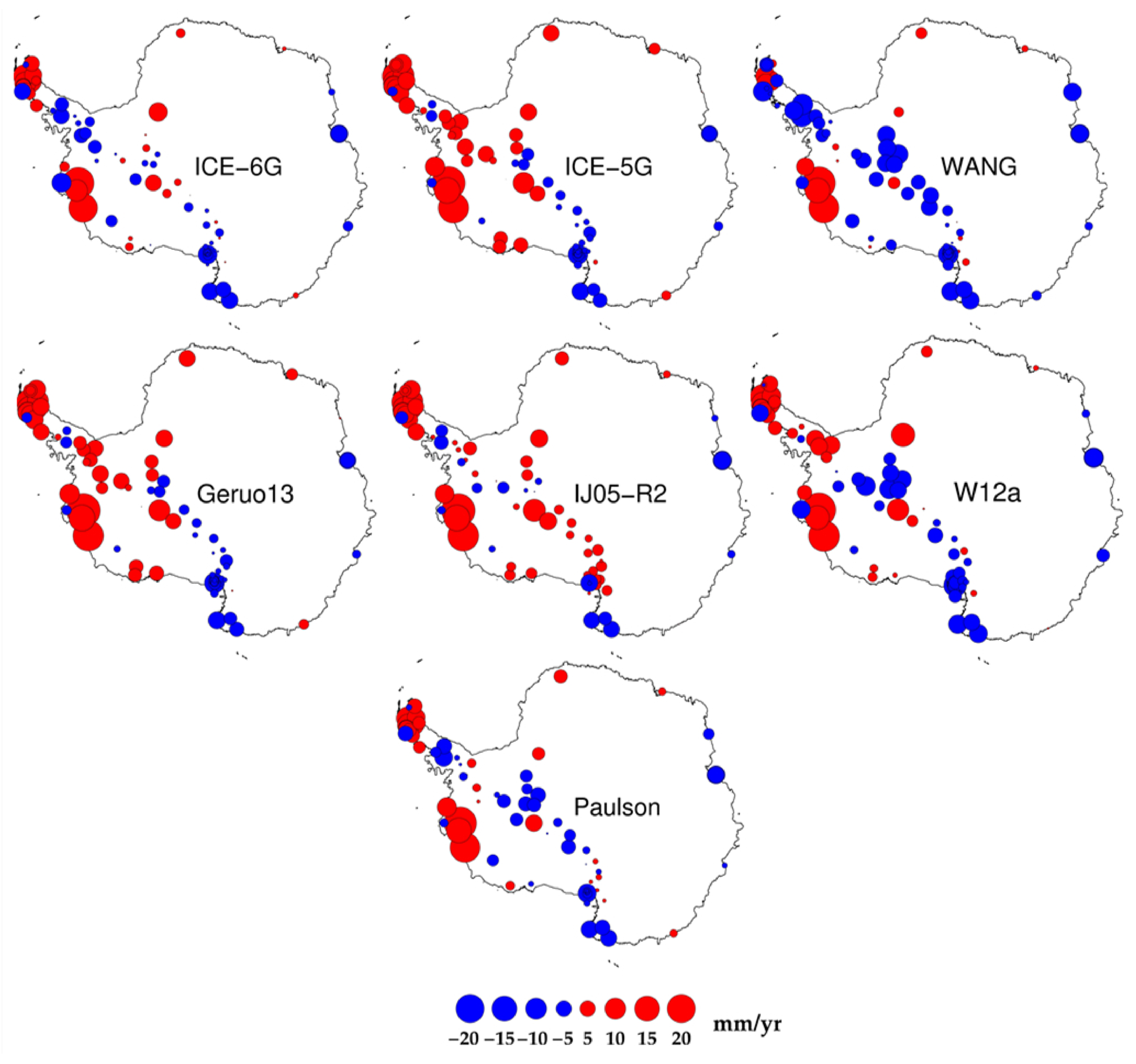
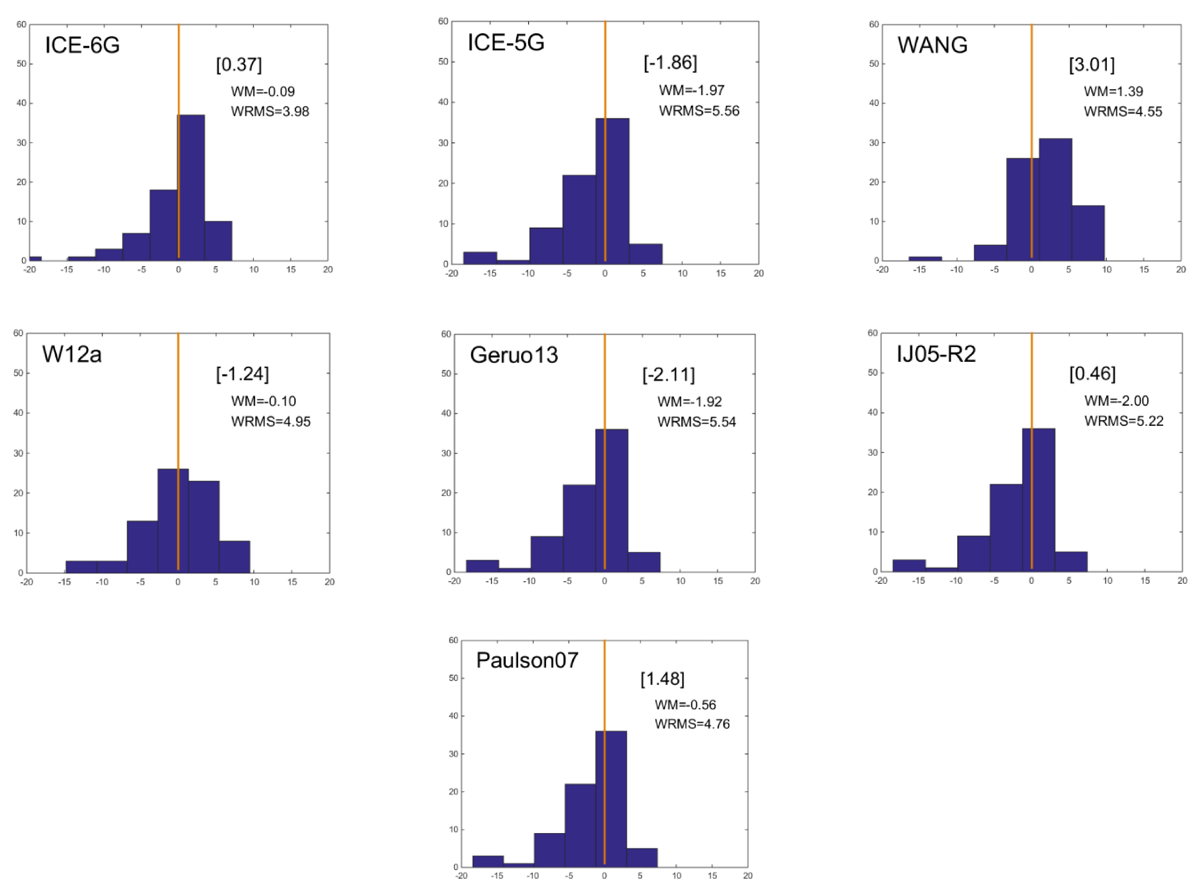
3.3. GIA Assessment
4. Discussion
5. Conclusions
- After applying an AIC noise analysis and ICA filtering, the maximum GPS velocity difference is up to 4.0 mm yr−1, the mean difference is 0.4 mm yr−1, and the velocity differences at 30% (24) of the stations are greater than ±0.4 mm yr−1.
- After applying ICA filtering and noise analysis, the weighted means of the residuals between most of the GIA model-predicted and GPS-observed uplift velocities decrease in most regions. On the Filchner–Ronne Ice Shelf, the GPS-observed velocities and the GIA model-predicted velocities are consistent. In East Antarctica, vertical motions are nonsignificant, and GIA and ice loading have small impacts on this area.
- For all 79 stations, the weight root mean squares are reduced, which means that the raw GPS velocities are affected by local effects. After applying the ICA filter and noise analysis, the local effects are depressed, and in the regions with relatively good consistency between the GPS-observed velocities and GIA model-predicted velocities, the consistency improves.
Supplementary Materials
Author Contributions
Funding
Data Availability Statement
Conflicts of Interest
References
- Wang, H.S.; Wu, P.; van der Wal, W. Using postglacial sea level, crustal velocities and gravity-rate-of-change to constrain the influence of thermal effects on mantle lateral heterogeneities. J. Geodyn. 2008, 46, 104–117. [Google Scholar] [CrossRef]
- Ivins, E.R.; James, T.S.; Wahr, J.; Schrama, E.J.O.; Landerer, F.W.; Simon, K.M. Antarctic contribution to sea level rise observed by GRACE with improved GIA correction. J. Geophys. Res. Solid Earth 2013, 118, 3126–3141. [Google Scholar] [CrossRef] [Green Version]
- Argus, D.F.; Blewitt, G.; Peltier, W.R.; Kreemer, C. Rise of the Ellsworth mountains and parts of the East Antarctic coast observed with GPS. Geophys. Res. Lett. 2011, 38. [Google Scholar] [CrossRef] [Green Version]
- Ke, H.; Li, F.; Zhang, S.K.; Ma, C.; Wang, A.X. The determination of absolute sea level changes of the Antarctic coast tidal gauges from 1994 to 2014 and its analysis. Chin. J. Geophys. 2016, 59, 3202–3210. [Google Scholar] [CrossRef]
- Peltier, W.R. Global glacial isostasy and the surface of the ice-age earth: The ice-5G (VM2) model and grace. Annu. Rev. Earth Planet. Sci. 2004, 32, 111–149. [Google Scholar] [CrossRef]
- Whitehouse, P.L.; Gomez, N.; King, M.A.; Wiens, D.A. Solid Earth change and the evolution of the Antarctic Ice Sheet. Nat. Commun. 2019, 10, 503. [Google Scholar] [CrossRef]
- Jia, L.L.; Wang, H.S.; Xiang, L.W.; Wu, P.; Li, F.; Shi, H.L. Effects of glacial isostatic adjustment on the estimate of ice mass balance over Antarctica and the uncertainties. Chin. J. Geophys. 2011, 54, 1466–1477. [Google Scholar] [CrossRef]
- Velicogna, I.; Wahr, J. Acceleration of Greenland ice mass loss in spring 2004. Nature 2006, 443, 329–331. [Google Scholar] [CrossRef] [Green Version]
- Sasgen, I.; Martinec, Z.; Fleming, K. Regional ice-mass changes and glacial-isostatic adjustment in Antarctica from GRACE. Earth Planet. Sci. Lett. 2007, 264, 391–401. [Google Scholar] [CrossRef] [Green Version]
- Riva, R.E.M.; Gunter, B.C.; Urban, T.J.; Vermeersen, B.L.A.; Lindenbergh, R.C.; Helsen, M.M.; Bamber, J.L.; de Wal, R.S.W.V.; van den Broeke, M.R.; Schutz, B.E. Glacial Isostatic Adjustment over Antarctica from combined ICESat and GRACE satellite data. Earth Planet. Sci. Lett. 2009, 288, 516–523. [Google Scholar] [CrossRef]
- Gunter, B.C.; Didova, O.; Riva, R.E.M.; Ligtenberg, S.R.M.; Lenaerts, J.T.M.; King, M.A.; van den Broeke, M.R.; Urban, T. Empirical estimation of present-day Antarctic glacial isostatic adjustment and ice mass change. Cryosphere 2014, 8, 743–760. [Google Scholar] [CrossRef] [Green Version]
- King, M.A.; Altamimi, Z.; Boehm, J.; Bos, M.; Dach, R.; Elosegui, P.; Fund, F.; Hernandez-Pajares, M.; Lavallee, D.; Cerveira, P.J.M.; et al. Improved Constraints on Models of Glacial Isostatic Adjustment: A Review of the Contribution of Ground-Based Geodetic Observations. Surv. Geophys. 2010, 31, 465–507. [Google Scholar] [CrossRef]
- Argus, D.F.; Peltier, W.R.; Drummond, R.; Moore, A.W. The Antarctica component of postglacial rebound model ICE-6G_C (VM5a) based on GPS positioning, exposure age dating of ice thicknesses, and relative sea level histories. Geophys. J. Int. 2014, 198, 537–563. [Google Scholar] [CrossRef]
- Peltier, W.R.; Argus, D.F.; Drummond, R. Space geodesy constrains ice age terminal deglaciation: The global ICE-6G_C (VM5a) model. J. Geophys. Res. Solid Earth 2015, 120, 450–487. [Google Scholar] [CrossRef] [Green Version]
- Wu, X.P.; Heflin, M.B.; Schotman, H.; Vermeersen, B.L.A.; Dong, D.A.; Gross, R.S.; Ivins, E.R.; Moore, A.; Owen, S.E. Simultaneous estimation of global present-day water transport and glacial isostatic adjustment. Nat. Geosci. 2010, 3, 642–646. [Google Scholar] [CrossRef]
- Dong, D.; Fang, P.; Bock, Y.; Webb, F.; Prawirodirdjo, L.; Kedar, S.; Jamason, P. Spatiotemporal filtering using principal component analysis and Karhunen-Loeve expansion approaches for regional GPS network analysis. J. Geophys. Res. Solid Earth 2006, 111, B03405. [Google Scholar] [CrossRef] [Green Version]
- Wdowinski, S.; Bock, Y.; Zhang, J.; Fang, P.; Genrich, J. Southern California Permanent GPS Geodetic Array: Spatial filtering of daily positions for estimating coseismic and postseismic displacements induced by the 1992 Landers earthquake. J. Geophys. Res. Solid Earth 1997, 102, 18057–18070. [Google Scholar] [CrossRef]
- Serpelloni, E.; Faccenna, C.; Spada, G.; Dong, D.A.; Williams, S.D.P. Vertical GPS ground motion rates in the Euro-Mediterranean region: New evidence of velocity gradients at different spatial scales along the Nubia-Eurasia plate boundary. J. Geophys. Res. Solid Earth 2013, 118, 6003–6024. [Google Scholar] [CrossRef] [Green Version]
- Shen, Y.Z.; Li, W.W.; Xu, G.C.; Li, B.F. Spatiotemporal filtering of regional GNSS network’s position time series with missing data using principle component analysis. J. Geod. 2014, 88, 1–12. [Google Scholar] [CrossRef]
- He, X.X.; Hua, X.H.; Yu, K.G.; Xuan, W.; Lu, T.D.; Zhang, W.; Chen, X. Accuracy enhancement of GPS time series using principal component analysis and block spatial filtering. Adv. Space Res. 2015, 55, 1316–1327. [Google Scholar] [CrossRef]
- Li, W.W.; Shen, Y.Z.; Li, B.F. Weighted spatiotemporal filtering using principal component analysis for analyzing regional GNSS position time series. Acta Geod. Geophys. 2015, 50, 419–436. [Google Scholar] [CrossRef] [Green Version]
- Yuan, L.G.; Ding, X.L.; Chen, W.; Simon, K.; Chan, S.B.; Hung, P.S.; Chau, K.T. Characteristics of daily position time series from the Hong Kong GPS fiducial network. Chin. J. Geophys. 2008, 51, 1372–1384. [Google Scholar] [CrossRef]
- Hyvarinen, A.; Oja, E. Independent component analysis: Algorithms and applications. Neural Netw. 2000, 13, 411–430. [Google Scholar] [CrossRef] [Green Version]
- Ming, F.; Yang, Y.X.; Zeng, A.M.; Zhao, B. Spatiotemporal filtering for regional GPS network in China using independent component analysis. J. Geod. 2017, 91, 419–440. [Google Scholar] [CrossRef]
- Li, W.H.; Li, F.; Zhang, S.K.; Lei, J.T.; Zhang, Q.C.; Yuan, L.X. Spatiotemporal Filtering and Noise Analysis for Regional GNSS Network in Antarctica Using Independent Component Analysis. Remote Sens. 2019, 11, 386. [Google Scholar] [CrossRef] [Green Version]
- He, X.X.; Bos, M.S.; Montillet, J.P.; Fernandes, R.; Melbourne, T.; Jiang, W.P.; Li, W.D. Spatial Variations of Stochastic Noise Properties in GPS Time Series. Remote Sens. 2021, 13, 4534. [Google Scholar] [CrossRef]
- Zhang, J.; Bock, Y.; Johnson, H.; Fang, P.; Williams, S.; Genrich, J.; Wdowinski, S.; Behr, J. Southern California Permanent GPS Geodetic Array: Error analysis of daily position estimates and site velocities. J. Geophys. Res. Solid Earth 1997, 102, 18035–18055. [Google Scholar] [CrossRef]
- Mao, A.L.; Harrison, C.G.A.; Dixon, T.H. Noise in GPS coordinate time series. J. Geophys. Res. Solid Earth 1999, 104, 2797–2816. [Google Scholar] [CrossRef] [Green Version]
- Bogusz, J.; Klos, A. On the significance of periodic signals in noise analysis of GPS station coordinates time series. GPS Solut. 2016, 20, 655–664. [Google Scholar] [CrossRef] [Green Version]
- Thomas, I.D.; King, M.A.; Bentley, M.J.; Whitehouse, P.L.; Penna, N.T.; Williams, S.D.P.; Riva, R.E.M.; Lavallee, D.A.; Clarke, P.J.; King, E.C.; et al. Widespread low rates of Antarctic glacial isostatic adjustment revealed by GPS observations. Geophys. Res. Lett. 2011, 38, L22302. [Google Scholar] [CrossRef] [Green Version]
- Nield, G.A.; Barletta, V.R.; Bordoni, A.; King, M.A.; Whitehouse, P.L.; Clarke, P.J.; Domack, E.; Scambos, T.A.; Berthier, E. Rapid bedrock uplift in the Antarctic Peninsula explained by viscoelastic response to recent ice unloading. Earth Planet. Sci. Lett. 2014, 397, 32–41. [Google Scholar] [CrossRef]
- Martin-Espanol, A.; King, M.A.; Zammit-Mangion, A.; Andrews, S.B.; Moore, P.; Bamber, J.L. An assessment of forward and inverse GIA solutions for Antarctica. J. Geophys. Res. Solid Earth 2016, 121, 6947–6965. [Google Scholar] [CrossRef] [PubMed] [Green Version]
- Liu, B.; King, M.; Dai, W.J. Common mode error in Antarctic GPS coordinate time-series on its effect on bedrock-uplift estimates. Geophys. J. Int. 2018, 214, 1652–1664. [Google Scholar] [CrossRef]
- Whitehouse, P.L.; Bentley, M.J.; Le Brocq, A.M. A deglacial model for Antarctica: Geological constraints and glaciological modelling as a basis for a new model of Antarctic glacial isostatic adjustment. Quat. Sci. Rev. 2012, 32, 1–24. [Google Scholar] [CrossRef]
- Whitehouse, P.L.; Bentley, M.J.; Milne, G.A.; King, M.A.; Thomas, I.D. A new glacial isostatic adjustment model for Antarctica: Calibrated and tested using observations of relative sea-level change and present-day uplift rates. Geophys. J. Int. 2012, 190, 1464–1482. [Google Scholar] [CrossRef] [Green Version]
- Geruo, A.; Wahr, J.; Zhong, S. Computations of the viscoelastic response of a 3-D compressible Earth to surface loading: An application to Glacial Isostatic Adjustment in Antarctica and Canada. Geophys. J. Int. 2013, 192, 557–572. [Google Scholar] [CrossRef]
- Paulson, A.; Zhong, S.J.; Wahr, J. Limitations on the inversion for mantle viscosity from postglacial rebound. Geophys. J. Int. 2007, 168, 1195–1209. [Google Scholar] [CrossRef] [Green Version]
- Bar-Sever, Y.E.; Kroger, P.M.; Borjesson, J.A. Estimating horizontal gradients of tropospheric path delay with a single GPS receiver. J. Geophys. Res. Solid Earth 1998, 103, 5019–5035. [Google Scholar] [CrossRef] [Green Version]
- Blewitt, G. Carrier Phase Ambiguity Resolution for the Global Positioning System Applied to Geodetic Baselines up to 2000 km. J. Geophys. Res.-Solid Earth Planets 1989, 94, 10187–10203. [Google Scholar] [CrossRef] [Green Version]
- Bertiger, W.; Desai, S.D.; Haines, B.; Harvey, N.; Moore, A.W.; Owen, S.; Weiss, J.P. Single receiver phase ambiguity resolution with GPS data. J. Geod. 2010, 84, 327–337. [Google Scholar] [CrossRef]
- Beavan, J. Noise properties of continuous GPS data from concrete pillar geodetic monuments in New Zealand and comparison with data from U.S. deep drilled braced monuments. J. Geophys. Res. Solid Earth 2005, 110, B08410. [Google Scholar] [CrossRef]
- Bos, M.S.; Fernandes, R.M.S.; Williams, S.D.P.; Bastos, L. Fast error analysis of continuous GNSS observations with missing data. J. Geod. 2013, 87, 351–360. [Google Scholar] [CrossRef] [Green Version]
- Schneider, T. Analysis of incomplete climate data: Estimation of mean values and covariance matrices and imputation of missing values. J. Clim. 2001, 14, 853–871. [Google Scholar] [CrossRef]
- Hyvarinen, A. Fast and robust fixed-point algorithms for independent component analysis. IEEE Trans. Neural Netw. 1999, 10, 626–634. [Google Scholar] [CrossRef] [Green Version]
- Peres-Neto, P.R.; Jackson, D.A.; Somers, K.M. How many principal components? stopping rules for determining the number of non-trivial axes revisited. Comput. Stat. Data Anal. 2005, 49, 974–997. [Google Scholar] [CrossRef]
- Agnew, D.C. Realistic Simulations of Geodetic Network Data: The Fakenet Package. Seismol. Res. Lett. 2013, 84, 426–432. [Google Scholar] [CrossRef]
- Akaike, H. New Look at Statistical-Model Identification. IEEE Trans. Autom. Control 1974, 19, 716–723. [Google Scholar] [CrossRef]
- Groh, A.; Ewert, H.; Scheinert, M.; Fritsche, M.; Rulke, A.; Richter, A.; Rosenau, R.; Dietrich, R. An investigation of Glacial Isostatic Adjustment over the Amundsen Sea sector, West Antarctica. Glob. Planet. Chang. 2012, 98–99, 45–53. [Google Scholar] [CrossRef]
- Barletta, V.R.; Bevis, M.; Smith, B.E.; Wilson, T.; Brown, A.; Bordoni, A.; Willis, M.; Khan, S.A.; Rovira-Navarro, M.; Dalziel, I.; et al. Observed rapid bedrock uplift in Amundsen Sea Embayment promotes ice-sheet stability. Science 2018, 360, 1335–1339. [Google Scholar] [CrossRef] [Green Version]
- Schroder, L.; Horwath, M.; Dietrich, R.; Helm, V.; van den Broeke, M.R.; Ligtenberg, S.R.M. Four decades of Antarctic surface elevation changes from multi-mission satellite altimetry. Cryosphere 2019, 13, 427–449. [Google Scholar] [CrossRef] [Green Version]
- Zhang, B.J.; Wang, Z.M.; Li, F.; An, J.C.; Yang, Y.D.; Liu, J.B. Estimation of present-day glacial isostatic adjustment, ice mass change and elastic vertical crustal deformation over the Antarctic ice sheet. J. Glaciol. 2017, 63, 703–715. [Google Scholar] [CrossRef] [Green Version]
- Dziewonski, A.M.; Anderson, D.L. Preliminary Reference Earth Model. Phys. Earth Planet. Inter. 1981, 25, 297–356. [Google Scholar] [CrossRef]
- Sasgen, I.; Konrad, H.; Ivins, E.R.; Van den Broeke, M.R.; Bamber, J.L.; Martinec, Z.; Klemann, V. Antarctic ice-mass balance 2003 to 2012: Regional reanalysis of GRACE satellite gravimetry measurements with improved estimate of glacial-isostatic adjustment based on GPS uplift rates. Cryosphere 2013, 7, 1499–1512. [Google Scholar] [CrossRef] [Green Version]
- An, M.J.; Wiens, D.A.; Zhao, Y.; Feng, M.; Nyblade, A.A.; Kanao, M.; Li, Y.S.; Maggi, A.; Leveque, J.J. S-velocity model and inferred Moho topography beneath the Antarctic Plate from Rayleigh waves. J. Geophys. Res. Solid Earth 2015, 120, 359–383. [Google Scholar] [CrossRef]
- Van der Wal, W.; Whitehouse, P.L.; Schrama, E.J.O. Effect of GIA models with 3D composite mantle viscosity on GRACE mass balance estimates for Antarctica. Earth Planet. Sci. Lett. 2015, 414, 134–143. [Google Scholar] [CrossRef] [Green Version]
- King, M.A.; Bingham, R.J.; Moore, P.; Whitehouse, P.L.; Bentley, M.J.; Milne, G.A. Lower satellite-gravimetry estimates of Antarctic sea-level contribution. Nature 2012, 491, 586–589. [Google Scholar] [CrossRef]
- Nield, G.A.; Whitehouse, P.L.; King, M.A.; Clarke, P.J. Glacial isostatic adjustment in response to changing Late Holocene behaviour of ice streams on the Siple Coast, West Antarctica. Geophys. J. Int. 2016, 205, 1–21. [Google Scholar] [CrossRef] [Green Version]
- Wolstencroft, M.; King, M.A.; Whitehouse, P.L.; Bentley, M.J.; Nield, G.A.; King, E.C.; McMillan, M.; Shepherd, A.; Barletta, V.; Bordoni, A.; et al. Uplift rates from a new high-density GPS network in Palmer Land indicate significant late Holocene ice loss in the southwestern Weddell Sea. Geophys. J. Int. 2015, 203, 737–754. [Google Scholar] [CrossRef] [Green Version]
- Zhao, C.; King, M.A.; Watson, C.S.; Barletta, V.R.; Bordoni, A.; Dell, M.; Whitehouse, P.L. Rapid ice unloading in the Fleming Glacier region, southern Antarctic Peninsula, and its effect on bedrock uplift rates. Earth Planet. Sci. Lett. 2017, 473, 164–176. [Google Scholar] [CrossRef] [Green Version]
- Heeszel, D.S.; Wiens, D.A.; Anandakrishnan, S.; Aster, R.C.; Dalziel, I.W.D.; Huerta, A.D.; Nyblade, A.A.; Wilson, T.J.; Winberry, J.P. Upper mantle structure of central and West Antarctica from array analysis of Rayleigh wave phase velocities. J. Geophys. Res. Solid Earth 2016, 121, 1758–1775. [Google Scholar] [CrossRef] [Green Version]
- Boening, C.; Lebsock, M.; Landerer, F.; Stephens, G. Snowfall-driven mass change on the East Antarctic ice sheet. Geophys. Res. Lett. 2012, 39, L21501. [Google Scholar] [CrossRef]


| GIA | Max (mm yr−1) | Min (mm yr−1) | Mean (mm yr−1) | Std (mm yr−1) |
|---|---|---|---|---|
| ICE-6G | 13.50 | −2.20 | 0.71 | 1.15 |
| ICE-5G | 13.90 | −2.80 | 1.58 | 1.10 |
| WANG | 15.27 | −2.13 | 2.60 | 1.15 |
| W12a | 10.33 | −6.11 | 0.58 | 0.97 |
| Geruo13 | 15.00 | −2.70 | 1.34 | 1.19 |
| IJ05-R2 | 5.24 | −0.88 | 0.22 | 0.45 |
| Paulson | 12.46 | −1.98 | 1.50 | 1.07 |
| Regions/GIA | ICE6G | ICE5G | WANG | W12a | Geruo13 | IJ05R2 | Paulson | |
|---|---|---|---|---|---|---|---|---|
| a | 0.83 | −0.99 | 2.30 | 0.86 | −0.94 | −1.03 | 0.88 | |
| Antarctica | b | 0.78 | −1.04 | 2.25 | 0.86 | −0.99 | −1.08 | 0.93 |
| c | −0.48 | −0.69 | 2.10 | −0.45 | −0.75 | −0.84 | 0.63 | |
| a | 1.24 | 1.46 | 2.26 | 2.81 | 1.43 | −0.74 | 1.24 | |
| ROSS | b | 1.18 | 1.40 | 2.21 | 2.87 | 1.37 | −0.80 | 1.18 |
| c | 0.98 | 1.20 | 2.00 | 2.60 | 1.17 | −1.00 | 0.98 | |
| a | −4.58 | −7.96 | −1.32 | −5.31 | −7.68 | −7.04 | −5.39 | |
| NAP | b | −4.94 | −8.31 | −1.67 | −5.37 | −8.03 | −7.39 | −5.75 |
| c | −0.78 | −4.15 | 2.49 | −3.51 | −6.87 | −3.23 | −1.59 | |
| a | 2.50 | −1.73 | 4.24 | −2.53 | −1.65 | 0.33 | 1.83 | |
| SAP | b | 2.30 | −1.92 | 4.05 | −2.72 | −1.85 | 0.13 | 1.64 |
| c | 1.62 | −2.60 | 3.37 | −3.40 | −2.53 | −0.55 | 0.96 | |
| a | −0.99 | −6.69 | −5.13 | −2.56 | −6.61 | −5.98 | −6.56 | |
| ASE | b | −0.70 | −6.10 | −4.54 | −1.97 | −6.02 | −5.39 | −5.97 |
| c | −0.40 | −5.11 | −3.54 | −6.98 | −5.03 | −4.39 | −3.97 | |
| a | 0.69 | −0.49 | 2.10 | 1.05 | −0.51 | 0.27 | 0.53 | |
| EA | b | 0.66 | −0.52 | 2.06 | 1.05 | −0.55 | 0.24 | 0.50 |
| c | 0.44 | −0.74 | 1.84 | 0.80 | −0.77 | 0.02 | 0.28 | |
| a | 2.32 | −2.24 | 3.00 | 2.38 | −2.17 | 0.66 | 1.61 | |
| FRIS | b | 2.52 | −2.04 | 3.20 | 2.58 | −1.97 | 0.87 | 1.82 |
| c | 1.20 | −3.36 | 1.88 | 1.26 | −3.29 | −0.45 | 0.50 | |
| Regions/GIA | ICE6G | ICE5G | WANG | W12a | Geruo13 | IJ05R2 | Paulson | |
|---|---|---|---|---|---|---|---|---|
| a | 4.00 | 5.68 | 4.27 | 4.90 | 5.57 | 5.14 | 4.68 | |
| Antarctica | b | 4.03 | 5.99 | 4.45 | 5.14 | 5.88 | 5.40 | 4.94 |
| c | 3.73 | 3.93 | 4.05 | 3.72 | 3.84 | 3.45 | 3.37 | |
| a | 1.58 | 2.16 | 2.93 | 3.41 | 2.11 | 1.50 | 1.88 | |
| ROSS | b | 1.59 | 2.14 | 2.96 | 3.33 | 2.09 | 1.54 | 1.94 |
| c | 1.51 | 2.12 | 2.84 | 3.19 | 2.08 | 1.76 | 1.88 | |
| a | 6.56 | 9.65 | 4.55 | 7.28 | 9.40 | 8.64 | 7.33 | |
| NAP | b | 6.89 | 9.99 | 4.78 | 7.60 | 9.74 | 8.98 | 7.65 |
| c | 3.82 | 6.01 | 4.35 | 4.21 | 5.79 | 5.13 | 4.25 | |
| a | 3.15 | 3.43 | 5.60 | 4.08 | 3.38 | 2.56 | 3.62 | |
| SAP | b | 2.96 | 3.44 | 5.36 | 4.17 | 3.39 | 2.42 | 3.41 |
| c | 3.22 | 3.41 | 4.20 | 4.47 | 3.35 | 1.75 | 2.32 | |
| a | 5.67 | 8.78 | 7.65 | 6.09 | 8.72 | 8.34 | 8.60 | |
| ASE | b | 5.69 | 8.41 | 7.34 | 5.95 | 8.34 | 8.00 | 8.23 |
| c | 5.72 | 5.76 | 7.75 | 5.25 | 8.70 | 8.42 | 8.57 | |
| a | 1.43 | 1.87 | 2.74 | 1.77 | 1.83 | 1.67 | 1.79 | |
| EA | b | 1.46 | 1.87 | 2.76 | 1.76 | 1.84 | 1.64 | 1.79 |
| c | 2.27 | 3.19 | 3.03 | 2.77 | 3.11 | 3.10 | 2.87 | |
| a | 2.53 | 3.10 | 4.91 | 2.95 | 3.04 | 2.33 | 3.01 | |
| FRIS | b | 2.72 | 2.94 | 5.00 | 3.12 | 2.89 | 2.41 | 3.09 |
| c | 1.63 | 3.82 | 4.50 | 2.18 | 3.75 | 1.60 | 2.72 |
Publisher’s Note: MDPI stays neutral with regard to jurisdictional claims in published maps and institutional affiliations. |
© 2022 by the authors. Licensee MDPI, Basel, Switzerland. This article is an open access article distributed under the terms and conditions of the Creative Commons Attribution (CC BY) license (https://creativecommons.org/licenses/by/4.0/).
Share and Cite
Li, W.; Li, F.; Shum, C.K.; Shu, C.; Ming, F.; Zhang, S.; Zhang, Q.; Chen, W. Assessment of Contemporary Antarctic GIA Models Using High-Precision GPS Time Series. Remote Sens. 2022, 14, 1070. https://doi.org/10.3390/rs14051070
Li W, Li F, Shum CK, Shu C, Ming F, Zhang S, Zhang Q, Chen W. Assessment of Contemporary Antarctic GIA Models Using High-Precision GPS Time Series. Remote Sensing. 2022; 14(5):1070. https://doi.org/10.3390/rs14051070
Chicago/Turabian StyleLi, Wenhao, Fei Li, C.K. Shum, Chanfang Shu, Feng Ming, Shengkai Zhang, Qingchuan Zhang, and Wei Chen. 2022. "Assessment of Contemporary Antarctic GIA Models Using High-Precision GPS Time Series" Remote Sensing 14, no. 5: 1070. https://doi.org/10.3390/rs14051070
APA StyleLi, W., Li, F., Shum, C. K., Shu, C., Ming, F., Zhang, S., Zhang, Q., & Chen, W. (2022). Assessment of Contemporary Antarctic GIA Models Using High-Precision GPS Time Series. Remote Sensing, 14(5), 1070. https://doi.org/10.3390/rs14051070